Elekta Precise Table characteristics of IGRT remote table positioning

Abstract

Introduction. Cone beam CT is a powerful tool to ensure an optimum patient positioning in radiotherapy. When cone beam CT scan of a patient is acquired, scan data of the patient are compared and evaluated against a reference image set and patient position offset is calculated. Via the linac control system, the patient is moved to correct for position offset and treatment starts. This procedure requires a reliable system for movement of patient. In this work we present a new method to characterize the reproducibility, linearity and accuracy in table positioning. The method applies to all treatment tables used in radiotherapy. Material and methods. The table characteristics are investigated on our two recent Elekta Synergy Platforms equipped with Precise Table installed in a shallow pit concrete cavity. Remote positioning of the table uses the auto set-up (ASU) feature in the linac control system software Desktop Pro R6.1. The ASU is used clinically to correct for patient positioning offset calculated via cone beam CT (XVI)-software. High precision steel rulers and a USB-microscope has been used to detect the relative table position in vertical, lateral and longitudinal direction. The effect of patient is simulated by applying external load on the iBEAM table top. For each table position an image is exposed of the ruler and display values of actual table position in the linac control system is read out. The table is moved in full range in lateral direction (50 cm) and longitudinal direction (100 cm) while in vertical direction a limited range is used (40 cm). Results and discussion. Our results show a linear relation between linac control system read out and measured position. Effects of imperfect calibration are seen. A reproducibility within a standard deviation of 0.22 mm in lateral and longitudinal directions while within 0.43 mm in vertical direction has been observed. The usage of XVI requires knowledge of the characteristics of remote table positioning. It is our opinion that the method presented meets the requirements in high precision IGRT.

Cone beam CT is a wide spread method in radiotherapy to evaluate the patient position relative to reference position. The patient position offset calculated via XVI-software is minimized using ASU remote table positioning feature in the linac control system. This procedure requires a reliable remote table positioning system [1], [2].

To have full benefit from a cone beam CT system, it is important that the uncertainty in x-ray tube and kV image panel system in the detection of volume position offsets (<1 mm) as well as remote table positioning to correct for the detected volume offset (<1 mm) are small. Table position measurements for test and calibration are normally based on high precision steel rulers. The measurements are often made with reference to laser lines, light field cross wire, treatment room wall or floor. This method requires high degree of care to meet the requirements.

A method for determining the alignment accuracy over time of treatment tables has been presented [3]. In this work a new method to measure treatment table positioning performance is developed. The method is image based without mechanical interaction and allows to measure linearity and reproducibility in positioning relative to prescribed values of an accuracy <0.1 mm.

Material and methods

Table characteristics were studied on our recent installed Elekta Synergy Platforms, MRT 8511, serial no. 15 1495 (Ac1) and 15 1666 (Ac4) both equipped with Precise Table, MRT 5071, serial no. 12 5624 and 12 5783, respectively, installed in a shallow pit concrete cavity. The table tops were a product of medical intelligence, iBEAM®evo Couchtop EP, P10105-148, serial no. 02 1506 and 02 2982, respectively. Both accelerators were equipped with electronic portal imaging device and XVI. In addition, the linac control system software Desktop Pro R6.1 was installed on both accelerators.

A Cartesian X_s, Y_s, Z_s-coordinate system was fixed with respect to the treatment table support (s) system with Z_s-axis vertical and positive upwards. The X_s, Y_s-axes were in the horizontal plane with Y_s-axis intersecting both table eccentric and isocentric rotational axis and being positive away from the eccentric axis[4]. Thus, for eccentric rotation at 0°, the X_s-axis was in the table top lateral (lat) direction and Y_s-axis was in the longitudinal (long) direction. The origin was defined to be on the table isocentric axis at isocentre height with Z_s being the vertical (vert) position of table top.

To describe the position of the table top in the horizontal plane with the eccentric rotation at 0°, a reference point (I_t) was defined and located at the intersection point of table isocentric axis through half the width of the table top with table fully retracted away from isocentre. The coordinates of reference point I_t relative to s-system were denoted T_x, T_y and were identical to lateral and longitudinal table top position. For T_y=37 cm, the table isocentric axis was located at the edge of the table top.

The positioning was investigated in each of the three directions with table eccentric and isocentric rotation fixed at 0°. The remote table top positioning was controlled by the ASU feature in Desktop Pro R6.1 software. The same experimental program was carried out at both tables to get data of the table top positioning with less statistical uncertainty.

The table tops were rectangular with length and width of 200 cm and 53 cm, respectively. The maximum movements in the vertical, lateral and longitudinal directions were 110, 50 and 100 cm, respectively. However, the measurements were in the longitudinal and lateral directions performed in the full operational range while limited to 40 cm in vertical direction.

At the superior end of the table top, 80 kg of external load was applied and equally distributed over a length of 60 cm from the edge and symmetrical around the Y_s-axis at T_x=0.0 cm.

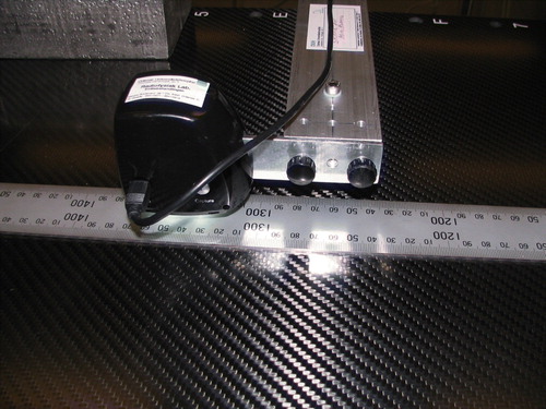
The position of the table top was measured using high precision stainless steel rulers of length 600 mm (No. 101E5E) and 2000 mm (No. 102H3E) both made by Shinwa (Shinwa Rulers Co., Ltd., http://211.121.171.178/english/shinwa.htm). For each table top position an image was exposed of the ruler using a USB-microscope. The longitudinal positioning was measured with the 2000 mm ruler attached to the table top in the length direction and aligned with the scale following the Y_s-axis at T_x=0.0 cm, see Figure 1. The lateral measurements were carried out with the 600 mm ruler attached to table top and positioned with its scale following the X_s-axis. In the vertical situation, the ruler was attached to the XVI flat panel with its scale vertical and intersected by the vertical plane through isocentric axis perpendicular to the Y_s-axis.

Figure 1.  Experimental set-up for the longitudinal measurements on Ac4 with the 2000 mm ruler aligned on the table top. The black housing is the USB-microscope from Spectrum Technologies, Inc. The 8 cm aluminium arm was mounted via two thumbscrews at the end of a 25×50 mm² massive aluminium bar of length 124 cm (weight 4.2 kg). A PTW MP3 water phantom was used as elevation stage for aluminium bar with the microscope mounted at the end.

A USB-microscope labeled Integrated Pest Management (IPM) Scope from Spectrum Technologies, Inc. (Spectrum Technologies, Inc., 12360 South Industrial Dr., East-Plainfield, 60585 Illinois, USA, www.specmeters.com) was used. The IPM Scope was connected to a personal computer via a USB-port. The image format was 480×640 pixels. The field of view used was approximately 6×8 mm² corresponding to a resolution of 0.013 mm/pixel.

The IPM scope was slightly modified to give a higher flexibility and robustness in the experimental set-up. An 8 cm aluminium arm with cross-section 3×25 mm² was attached by two screws to the cooling ribble inside the housing. An opening in the housing was made for the aluminium arm. Thus, 6.5 cm of the arm was sticking out the housing for attachment to additional holders.

In the longitudinal and lateral experimental set-ups the microscope was fixed to floor on an elevation stage. In the vertical set-up the microscope was attached to the table top. The alignment was checked before measurements by doing scans in the full range. The position of ruler and microscope were adjusted to achieve ruler parallel to scan direction and to ensure that the images of the ruler were suitable for position analysis afterwards. Also, the distance between microscope and ruler was adjusted to give well focused images. All images were exposed at largest field of view of the microscope.

The prescribed table top position was entered in the linac control system. The ASU button was pressed until the table clutch was activated. The clutch was activated when the prescribed value was identical with the position value read out from the control system also denoted as display position. If the display position was deviating from the prescribed position, a movement of the table top via ASU was possible until prescribed and display position were identical. Microscope images were taken of preselected table positions and stored on a personal computer. Each exposure were acquired by pressing the exposure button in the microscope IPM Scope software by mouse click. The images were calibrated and analyzed in software and table top positions were extracted from the images relative to the reference X_sY_sZ_s-coordinate system.

The images were handled in ImageJ (ImageJ, http://rsb.info.nih.gov/ij/) for stacking in video sequences and saving in the AVI-file format. The analyzes were carried out in Tracker (Tracker video, www.cabrillo.edu). In this software the image calibration was performed and the table positions coordinates were calculated. Both softwares can be downloaded from the Internet free of charge.

Results and discussion

We have observed that the movement to the final position takes place differently. In some cases, the table comes to correct position by moving one way, and in other cases overshooting have been observed. Also, table top oscillations around prescribed position with ±1 mm over many seconds have been discovered. In extreme cases, these oscillations never ended. However, by activating and deactivating the ASU button in turn, the table top positioning process was finished at final position. The way the table top is moving to correct position can be adjusted. The adjustments are complex primarily because a compromise between accurate positioning over long time and less accurate positioning over short time has to be taken.

In Figure 2–Figure 4 deviation data of table top positioning in three directions as function of display position are shown. The deviation was defined as display minus measured position. In the figures, the slope of the best linear fit to the data points is representing a systematic error in the position calibration. According to Elekta costumer acceptance tests a calibration within an accuracy of 4.0 mm/m in vertical direction is obtainable. Thus, the table top calibration could be improved for the vertical positioning of Ac4, Figure 2. Precise calibration is most important for patient set-up in a reference point followed by a certain prescribed movement to the position of treatment. For the clinical users of XVI and remote table positioning, the maximum movement in remote mode is 2 cm in each axis. Thus, the maximum error due to calibration is approximately 0.08 mm. Therefore, it is the standard deviations describing the size of random errors that concerns clinical users of XVI. It is seen that the standard deviation for vertical positioning is slightly higher than those found in lateral and longitudinal directions. In Table I, the key parameters of all measurements are listed. In the Elekta product data sheet, a standard deviation of 0.5 mm in each directions for remote table positioning for a typical operator was reported. The values found in this work are below their values.

Figure 2.  Deviation in vertical positioning on Ac1 and Ac4. Each marker represents a table top position measurement. The fully drawn line represents the best linear fit. The dashed lines are located two times the standard deviation away from linear fit. The table was positioned lateral at 0.0 cm, longitudinal at 70.0 cm, eccentric and isocentric table rotation at 0°. The external load was increased to 84 kg due to an addition weight from the aluminium rod holding the microscope. The vertical position was −20.0 cm, −15.0 cm, −10.0 cm to 10.0 cm in steps of 1.0 cm, 15.0 cm, 20.0 cm and return, in total 50 positions.

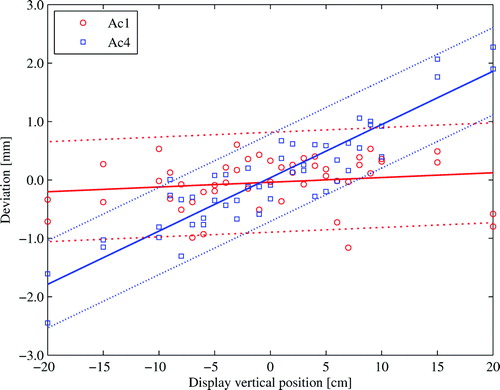
Figure 3.  Deviation in lateral positioning on Ac1 and Ac4. Each marker represents a table top position measurement. The fully drawn line represents the best linear fit. The dashed lines are located two times the standard deviation away from linear fit. The table was positioned vertical at −10.1 cm, longitudinal at 70.0 cm, eccentric and isocentric table rotation at 0°. The lateral position was varied from −25.0 cm to 25.0 cm in steps of 1.0 cm and return, in total 102 positions. Only 93 positions were measured on Ac1 due to limits for the remote positioning which did not allow remote movement from a position inside the range [−22.4;22.8] cm to a position outside.

Figure 4.  Deviation in longitudinal positioning on Ac1 and Ac4. Each marker represents a table top position measurement. The fully drawn line represents the best linear fit. The dashed lines are located two times the standard deviation away from linear fit. The table was positioned vertical at −10.1 cm, lateral at 0.0 cm, eccentric and isocentric table rotation at 0°. The longitudinal position was varied from 1.0 cm to 99.0 cm in steps of 1.0 cm and return, in total 198 positions.

Table I.  Analyzes of data presented in Figure 2–Figure 4. Slope is a quantity which characterizes the precision of calibration. Std (standard deviation) describes the uncertainty in the positioning.

Accelerator	Movement	Slope [mm/m]	Std [mm]
Ac1	Vert	0.8	0.43
	Lat	−2.2	0.17
	Long	0.1	0.22
Ac4	Vert	9.1	0.37
	Lat	−3.7	0.22
	Long	−2.7	0.20

We emphasize that in our experiments, the ASU button was pressed until the prescribed and display positions were identical. This means that the data we have presented in this work reflect the most optimal achievable. However, in clinical use the standard deviation might be slightly higher depending on the ASU operator because a difference between the prescribed and display positions is permitted within predefined tolerances.

Acknowledgements

Declaration of interest: The authors report no conflicts of interest. The authors alone are responsible for the content and writing of the paper.

References

- Cho Y, Moseley DJ, Siewerdsen JH, Jaffray DA. Accurate technique for complete geometric calibration of cone-beam computed tomography systems. Med Phys 2005; 32: 968–83
- Sharpe MB, Moseley DJ, Purdie TG, Islam M, Siewerdsen JH, Jaffray DA. The stability of mechanical calibration for a kV cone beam computed tomography system integrated with linear accelerator. Med Phys 2006; 33: 133–44
- Karger CP, Hartmann GH, Heeg P, Jäkel O. NOTE: A method for determining the alignment accuracy of the treatment table axis at an isocentric irradiation facility. Phys Med Biol 2001; 46: 19–26
- International Standard, International Electrotechnical Commission (IEC), IEC 61217, Geneva. Radiotherapy equipment-Coordinates, movements and scales; 2002.