Autodelineation of cervical cancers using multiparametric magnetic resonance imaging and machine learning

Abstract

Background: Tumour delineation is a challenging, time-consuming and complex part of radiotherapy planning. In this study, an automatic method for delineating locally advanced cervical cancers was developed using a machine learning approach.

Materials and methods: A method for tumour segmentation based on image voxel classification using Fisher?s Linear Discriminant Analysis (LDA) was developed. This was applied to magnetic resonance (MR) images of 78 patients with locally advanced cervical cancer. The segmentation was based on multiparametric MRI consisting of T2- weighted (T2w), T1-weighted (T1w) and dynamic contrast-enhanced (DCE) sequences, and included intensity and spatial information from the images. The model was trained and assessed using delineations made by two radiologists.

Results: Segmentation based on T2w or T1w images resulted in mean sensitivity and specificity of 94% and 52%, respectively. Including DCE-MR images improved the segmentation model?s performance significantly, giving mean sensitivity and specificity of 85?93%. Comparisons with radiologists? tumour delineations gave Dice similarity coefficients of up to 0.44.

Conclusion: Voxel classification using a machine learning approach is a flexible and fully automatic method for tumour delineation. Combining all relevant MR image series resulted in high sensitivity and specificity. Moreover, the presented method can be extended to include additional imaging modalities.

Introduction

Tumour delineation is an important step in radiotherapy planning and is today done manually by a radiation oncologist or a radiologist [1]. It is well known that the interobserver variability between radiologists can be large [2–4], and that intraobserver variability also occurs [5]. With the increasing use of multimodal imaging, the task of correctly identifying the tumour becomes more complex and potentially prone to human bias [6,7]. Computers can handle large amounts of data, and will, unlike a human observer, treat the images quickly and identically [8]. An automatic tumour segmentation method could therefore be a valuable and time saving tool for radiologists [6,9].

Methods for tumour segmentation include both machine learning techniques as well as methods specific for medical image segmentation [9,10]. No fully automatic delineation methods have been published for cervical cancers. Most studies, as recently reviewed by Ghose et al. [11], focus on delineating organs at risk, or use the manual delineation from treatment planning to autodelineate tumours in images acquired during treatment using registration algorithms [12]. Methods proposed for identifying tumours in the cervix tend to have a high degree of manual interaction [11,13].

An automatic method for tumour autodelineation should be robust, fast and not overly complex [6,10]. One method encompassing these criteria is the linear discriminant, Fisher’s Linear Discriminant Analysis (LDA) [14], a well-known supervised machine learning classifier [7], which can be trained to identify tumour and non-tumour voxels in medical images. Riches et al. [15] recently used this method to classify voxels as tumour or non-tumour in a study of prostate cancers. Furthermore, the nonlinear classifier Quadratic Discriminant Analysis (QDA) is very similar to LDA, and can be used to compare tumour delineations made by linear and nonlinear decision boundaries [7].

In this study, we considered a data set based on 78 patients with locally advanced cervical cancer. As magnetic resonance imaging (MRI) is considered the optimal imaging modality for these patients [12], we developed and evaluated a machine learning approach for tumour autodelineation based on multiparametric MRI consisting of T2-weighted (T2w), T1-weighted (T1w) and dynamic contrast-enhanced (DCE) sequences. We considered the two-class problem where voxels were identified as tumour or non-tumour and explored how MR images could be combined to provide accurate tumour segmentation. Both voxel intensity and spatial features of the images were used for the segmentation. Fisher’s LDA and the nonlinear QDA were used as voxel classifiers. Delineations made by two experienced radiologists represented the ground truth.

Materials and methods

Images and patients

The data set consisted of MR images from 78 patients with locally advanced cervical cancer, FIGO stages 1b through 4a, and an average tumour volume of 37 cm³ [16]. The study was approved by the Norwegian Regional Committee for Medical and Health Research Ethics, and written informed consent was obtained from all patients. All MR images were acquired in the period 2001–2004.

MRI was performed on a 1.5-T Signa Horizon LX tomograph (GE Medical Systems, Milwaukee, WI). All patients underwent T2w imaging (FSE; TR range, 4220–5380 ms; TE range, 83–85 ms; matrix size 512 × 512; in-plane resolution, 0.39 mm; slice thickness, 5 mm; slice gap, 1 mm), T1w imaging (FSE; 420–600 ms; 8.1–10.6 ms; 512 × 512; 0.39 mm; 5 mm; 1 mm) and DCE-MRI (T1w FSPGR with flip angle 90°; 80 ms; 3.4–3.6 ms; 256 × 256; 0.78 mm; 5 mm; 1 mm) prior to chemoradiotherapy [16]. The T2w and T1w images had 20 and 32 slices per patient, respectively, while the DCE-MRI series had 9 or 10 slices per patient.

The DCE-MRI series consisted of 1 pre-contrast image and between 12 and 15 post-contrast images per patient. The contrast agent Gd-DTPA (Magnetvist^®; Schering, Berlin, Germany) was manually administered as a fast bolus injection [16]. The first 11 post-contrast images were acquired with 15-s intervals, while the rest of the series was acquired at 1-min intervals. In the current framework, the 13 first time steps (pre-contrast image and the 12 first post-contrast images) were used in order to have the same number of time steps for all voxels in the data set.

The T2w images were used for tumour delineation by two experienced radiologists. Necrotic areas in tumours, if present, were included in the delineation. The delineations that the radiologists together agreed upon were assumed to represent the ground truth and were used to assess the performance of the automatic segmentation procedure.

Image pre-processing

Prior to voxel classification, the edges of the images were removed as shown in Figure 1(a). This reduced the size of the data set and removed irrelevant voxels, such as those including air around the patient. Removing the edges also gave a higher percentage of tumour voxels in the data set, resulting in better balance between the two voxel classes (tumour and non-tumour). Only the image slices in which the radiologists identified tumour tissue were used, further balancing the data set. The images for all 78 patients were combined into one large data set consisting of a total of 486 image slices, where each slice had three different MR representations (T2w, T1w and DCE-MRI). Twenty-seven percent of the voxels in the data set were tumour voxels, while 73% were non-tumour voxels. For analyses combining all three image types, the T2w and T1w images were downscaled to match the size of the DCE-MR images.

Figure 1. Conversion of the MR images into a data matrix X used for voxel classification. (a) Edges were removed from all images. (b) For the DCE-MRI series, each voxel was represented by the intensities of the 13 first time steps in the image series. (c) The T2w or T1w images were represented by either only their intensity, or by their intensity (dark grey) and the intensities of the eight closest neighbour voxels (light grey). (d) The data matrix X for the model based on T2w images with eight neighbours included, the T1w images with eight neighbours included and the 13 first DCE-MRI time steps.

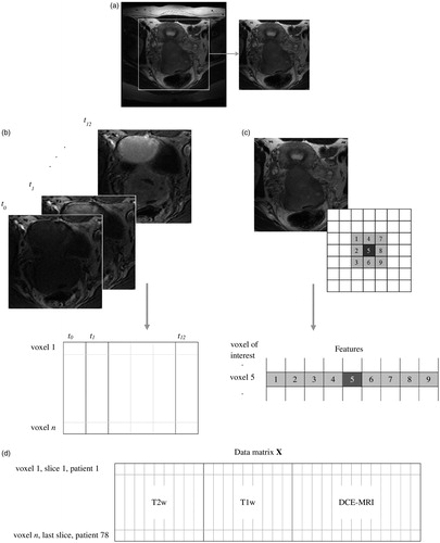
To compensate for varying image intensities between patients, we investigated autoscaling of the signal intensity of the images to mean zero and standard deviation one for each patient. For the DCE-MR images we autoscaled the entire series (all time steps) as one, to maintain the intensity increase between time steps.

Image feature extraction

The data matrix was constructed as illustrated in Figure 1. For the T2w and T1w images, each voxel was represented by its intensity. To retain information on the spatial relationships between voxels, we also included the eight closest neighbour voxels for each voxel of interest, resulting in nine intensity features for each voxel [17]. For the DCE-MRI, each voxel was represented by its time–intensity curve, that is, the intensities measured at each of the 13 time points. The data matrix shown in Figure 1(d) (labelled X), based on T2w and T1w images using eight neighbours and the 13 first time steps of the DCE-MRI series (no neighbours) therefore consisted of 31 columns (features) and one row for each voxel in the 486 slices. For autodelineations based on T2w and T1w images alone, the higher spatial resolution of these images was used rather than the downscaled versions.

Linear and quadratic discriminant analysis

Fisher’s LDA [14] seeks to find a line separating two (or more) groups in the data set by minimizing scatter within the groups while maximizing the scatter between the groups [7,14].

LDA models classifying voxels in the data matrices as tumour or non-tumour were trained using the radiologists’ contour. The classification results provided probability maps giving the probability of each voxel belonging to the tumour [18]. The probability maps were converted to binary segmentations by setting the probability threshold to 50%, implying that all voxels with a probability greater than 50% were assigned to the tumour. Finally, we employed in-plane morphological opening on these binary masks to remove small islets less than 100 voxels large.

QDA is a nonlinear classification method very similar to LDA [7], where a quadratic, rather than a linear, boundary is found between the classes. We used QDA on the most promising data matrix from the LDA tests to assess the added value of using a nonlinear classifier.

Validation and statistical analysis

Leave-one-out cross-validation was used to estimate model performance on a new set of images not included in the model training [10]. All images from one patient were removed from the data set, and the LDA/QDA model was trained on the remaining images [7,17]. The resulting LDA/QDA model was then used for segmentation of the images from the left-out patient. This was repeated until all the patients had been left out once and the model performance was assessed. This validation method mimics the situation in the clinic, where a new patient will be diagnosed using a model trained on images from earlier patients. All presented results have been leave-one-out cross-validated.

To evaluate the overlap between the masks made by the radiologists (ground truth) and the mask produced by the LDA/QDA classification model, we used the Dice similarity coefficient (DSC) [9,19] and the kappa statistics K [5,20]. Sensitivity (Sens) and specificity (Spec) were also calculated to assess model performance for classifying each of the two voxel groups (tumour and non-tumour). Finally, the area under the Receiver Operating Characteristic (ROC) curve (AUC) was calculated for each model [21].

After verifying the normality assumptions, N-way ANOVA with significance level p < 0.05 was used to test the effect of image type (T2w, T1w or DCE-MRI), pre-processing (autoscaling or no pre-processing) and spatial information (eight neighbours or no neighbours) on the five-model performance measures (DSC, Sens, Spec, K and AUC). Main effects and two-factor interactions were tested.

Calculations

All calculations and LDA classifications were conducted in MATLAB (v8.5, R2015a, The Mathworks Inc., Natick, MA). QDA and statistical analysis of variance tests were conducted in the MATLAB Statistics and Machine Learning Toolbox (v10.0).

Results

As seen in Table 1, all models based on T2w images, T1w images or a combination of these two image types, had DSC values between 0.18 and 0.20 and K values between 0.14 and 0.17, indicating low but better than chance agreement with the radiologists’ masks. These models had high sensitivity (0.91–0.95), but low specificity (0.50–0.54). Tables 1 and 2 show a significant increase in most performance measures when T1w images were used instead of or in addition to the T2w images.

Table 1. Performance measures for LDA classification models based on different combinations of feature vectors derived from T2w, T1w or DCE-MR images.

Images	Pre-processing	Neighbours	DSC	Sens	Spec	AUC	K
T2w	None	0	0.18	0.91	0.51	0.65	0.14
T2w	Autoscaled	0	0.18	0.93	0.53	0.73	0.14
T2w	None	8	0.18	0.91	0.52	0.66	0.15
T2w	Autoscaled	8	0.18	0.92	0.54	0.67	0.15
T1w	None	0	0.19	0.94	0.52	0.70	0.17
T1w	Autoscaled	0	0.19	0.95	0.52	0.73	0.16
T1w	None	8	0.20	0.94	0.52	0.71	0.17
T1w	Autoscaled	8	0.19	0.95	0.53	0.75	0.16
T2w + T1w	None	0	0.19	0.93	0.52	0.72	0.16
T2w + T1w	Autoscaled	0	0.19	0.95	0.53	0.75	0.16
T2w + T1w	None	8	0.20	0.93	0.53	0.73	0.17
T2w + T1w	Autoscaled	8	0.19	0.95	0.54	0.76	0.17
DCE	None	0	0.42	0.92	0.85	0.84	0.39
DCE	Autoscaled	0	0.43	0.92	0.85	0.85	0.41
T2w + DCE	None	0	0.41	0.93	0.84	0.85	0.38
T2w + DCE	Autoscaled	0	0.42	0.93	0.84	0.85	0.39
T2w + DCE	None	T2w: 8 DCE: 0	0.41	0.93	0.84	0.85	0.39
T2w + DCE	Autoscaled	T2w: 8 DCE: 0	0.41	0.93	0.84	0.85	0.39
T1w + DCE	None	0	0.43	0.93	0.85	0.86	0.41
T1w + DCE	Autoscaled	0	0.44	0.93	0.85	0.87	0.41
T1w + DCE	None	T1w: 8 DCE: 0	0.43	0.93	0.85	0.86	0.41
T1w + DCE	Autoscaled	T1w: 8 DCE: 0	0.44	0.94	0.85	0.87	0.42
T2w + T1w + DCE	None	0	0.43	0.93	0.85	0.86	0.40
T2w + T1w + DCE	Autoscaled	0	0.43	0.93	0.85	0.87	0.41
T2w + T1w + DCE	None	T2w, T1w: 8 DCE: 0	0.43	0.93	0.85	0.86	0.41
T2w + T1w + DCE	Autoscaled	T2w, T1w: 8 DCE: 0	0.44	0.94	0.85	0.87	0.42

LDA: Linear Discriminant Analysis; DSC: Dice similarity coefficient; Sens: sensitivity; Spec: specificity; AUC: area under curve; K: kappa statistic. Values averaged over all patients are shown.

The images were either autoscaled or not pre-processed.

The column ‘Neighbours’ indicates how many of the neighbour voxel intensities were used as spatial features, here either none or the eight closest.

Table 2. p Values from N-way ANOVA for the effects of the factors image type, pre-processing and spatial information on the classification performance measures.

Factor or interaction	DSC	Sens	Spec	AUC	K
T1w	>0.001	>0.001	–	>0.001	>0.001
DCE-MRI	>0.001	–	>0.001	>0.001	>0.001
Pre-processing	–	>0.001	>0.001	0.003	–
Neighbours	–	–	0.03	–	–
T2w * T1w	–	0.04	0.04	–	–
T2w * DCE-MRI	–	–	0.03	–	–
T1w * DCE-MRI	–	>0.001	–	0.005	–
DCE-MRI * pre-processing	0.005	0.002	>0.001	0.02	0.009
DCE-MRI * neighbours	–	–	>0.001	–	–

–, not significant (p > 0.05). DSC: Dice similarity coefficient; Sens: sensitivity; Spec: specificity; AUC: area under curve; K: kappa statistic. Only factors and interactions with significant effect on at least one of the performance measures are shown. All other factors or interactions were not significant (p > 0.05).

Tables 1 and 2 show that inclusion of the DCE-MRI features had a significant effect on all performance measures except sensitivity. Models including DCE-MRI features had significantly higher values of DSC (0.41–0.44), K (0.38–0.42), AUC (0.84–0.87) and specificity (0.92–0.94) than models based solely on T1w and T2w images, indicating improvement in model performance. For these DCE-MRI based models, sensitivity and specificity were more similar (0.84–0.95), showing that the models classified each group of voxels (tumour or non-tumour) equally well.

Pre-processing by autoscaling the images had a small but significant positive effect on sensitivity, specificity and AUC (Tables 1 and 2). Interaction between DCE-MRI and autoscaling had a significant positive effect on all performance measures, indicating that the DCE-MR images benefitted more from pre-processing than the T2w and T1w images. This could be due to a larger intensity variation between patients when contrast agent is used. The specificity increased when spatial information was included (Tables 1 and 2).

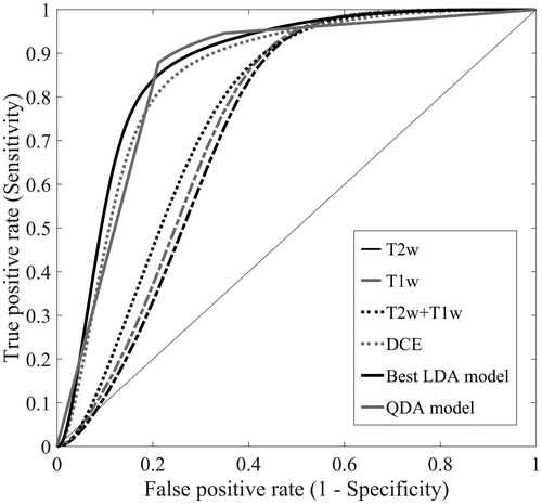
A selection of ROC curves is shown in Figure 2. The area under the curve was larger for the models based on DCE-MRI than for models based solely on T2w and/or T1w images (see Table 1). The best performing LDA was model based on all image types with eight neighbours included, using autoscaling as image pre-processing. A QDA model was fitted to the same data set, giving DSC = 0.32, Sens = 0.98, Spec = 0.72, AUC = 0.91 and K = 0.30. As the ROC curve in Figure 2 shows, this model had similar performance to the LDA model, but was more dependent on the choice of threshold between the two voxel classes. However, the potential gain in performance by using the nonlinear QDA instead of LDA was very small.

Figure 2. ROC curves for five LDA models based on either T2w images, T1w images, T2w and T1w images, DCE-MR images or all three image types combined. The ROC curves represent the LDA model with the highest AUC for each category. The curve labelled ‘Best LDA model’ represents the LDA model based on all image types with eight neighbours included series (Table 1, bold), using autoscaling as image pre-processing. This model had the highest overall performance. The sixth curve labelled ‘QDA model’ represents the QDA model based on the same image data set as the best LDA model.

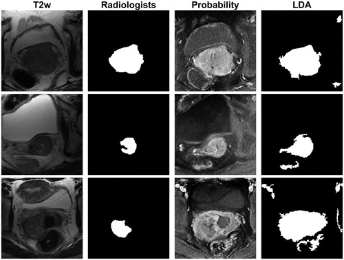
Figure 3 shows a scatter plot of average DSC, Sens, Spec and K for each patient from the best performing model (see Table 1, bold row and Figure 2 ‘Best LDA model’ for ROC curve). All patients had sensitivity and specificity values above 0.6, and most patients (83%) had DSC and K values between 0.2 and 0.6. However, Figure 3 also shows that model performance varied from patient to patient. For example, the average DSC for each patient varied from 0.09 to 0.70. To further illustrate this variation, LDA model classifications from selected slices from three different patients are shown together with the radiologists’ masks in Figure 4. For the first image slice, the agreement between the radiologists’ mask and the LDA binary mask was good (DSC = 0.82). The second row shows an image slice with intermediate agreement between the radiologists and the LDA binary mask (DSC = 0.57), where the LDA model delineates a too large tumour compared to the radiologists. Lower agreement between the radiologists and the LDA binary mask was obtained for the last slice (DSC = 0.31). In this case, the model identified many voxels with over 50% probability of belonging to the tumour. However, even in the case of the last slice regions of high tumour probability coincided well with the radiologists’ assessment, but too many other structures were included in the final delineation.

Figure 3. Scatter plot of the Dice similarity coefficient (DSC), kappa (K), sensitivity (Sens) and specificity (Spec) averaged for each patient for the leave-one-out cross-validated LDA model based on all image types with eight neighbour voxels included, using autoscaling as image pre-processing. This model is labelled ‘Best LDA model’ in Figure 2 (see also Table 1, bold).

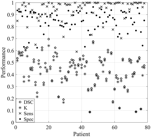
Figure 4. The T2w image (first column) and the radiologists’ mask (second column) for image slices from three different patients. The tumour probability maps (third column) and the binary masks (fourth column) derived from the LDA model based on all image types with eight neighbour voxels included, using autoscaling as image pre-processing (Table 1, bold). In the tumour probability maps, black and white indicate 0% and 100% predicted probability, respectively, of the voxel belonging to the tumour. The agreement between the radiologists’ mask and the LDA binary mask given by the Dice similarity coefficient (DSC) was for these image slices 0.82 (first row), 0.57 (middle row) and 0.31 (last row).

Discussion

A machine learning method for automatic segmentation of cervical cancer tumours by combining information from multiparametric MRI was developed and evaluated using delineations made by two experienced radiologists. DCE-MRI features were more successful at identifying tumours than the T2w or T1w images, either combined or separately. The DCE-MRI series provides information on the vasculature of the tumours, and emphasizes tissue perfusion and blood vessel permeability [22]. Our results indicated that the vascular properties of the tumour and non-tumour tissue were different. It should also be noted that including T1w images significantly improved the model delineation. This is in line with a study by Akita et al. [23], who found that contrast-enhanced T1w images was preferable for manual delineation over T2w images for cervical cancer patients with stages 1B or higher.

The LDA models giving the best tumour segmentation performance had overall sensitivity and specificity values in the range 0.84–0.95. Thus, tumour and non-tumour voxels were predicted equally well. The best LDA model had a K value of 0.42, indicating fair agreement with the radiologists’ assessment [5], and all models based on the DCE-MRI series had K values between 0.38 and 0.42. The inter-rater agreements between radiologists reported in literature vary. For example, Hricak et al. [5] compared evaluations from four different radiologists on 152 patients with early invasive cervical cancer, where the radiologists gave the images scores representing tumour visibility. They found a multi-rater kappa value of 0.32 for tumour visualization, demonstrating disagreement between the radiologists. Dimopoulos et al. [2] compared delineation made by two observers. They used different measures of agreement than our study, but also found large variations in the interobserver agreement. Even though published studies tend to compare visibility scores rather than the actual delineated volumes, they still demonstrate relatively large disagreement between observers.

No automatic segmentation methods for cervical cancers have been published [11]. For prostate cancer, however, several autodelineation algorithms have been presented [15,24]. Similar to the current study, Riches et al. [15] recently used LDA on multiparametric MRI to classify voxels as belonging to the tumour, the peripheral zone or the central gland of the prostate. Their results were comparable to ours, with AUC of up to 0.88. In prostate cancer studies, atlases are often used to segment the prostate itself, before identifying the intraprostatic tumour lesions. As cervical cancers tend not to be constrained to the cervix, this technique is less relevant here. A variety of methods for voxel classification and image pre-processing has been used in the literature [11]. In our study, we saw only minor potential benefits of using the nonlinear QDA classifier instead of LDA. Nor were the delineations improved by using other pre-prosessing methods such as contrast-limited adaptive histogram equalization for correction of magnetic field bias or principal component analysis for reduction of noise in the time series (data not shown).

The segmentation procedure described in this study has certain strengths. LDA is a fast and robust technique that does not require optimization. The method provides probability maps rather than strict binary segmentations [18,21]. Thus, in the case of tumour segmentation, the LDA classification can be illustrated as tumour probability maps. These maps may be more useful for a radiologist than a binary segmentation, as they illustrate the probability of each voxel belonging to the tumour. As seen here, regions of high tumour probability coincided well with the regions selected by the radiologists. Based on these maps, the radiologist can identify voxels close to the probability threshold between tumour and non-tumour, and give them special attention. Although the method presented here was fully automatic, it could be modified to a semi-automatic method, for example by allowing the radiologist to choose a region of interest (ROI), to tune the probability threshold for tumour voxels in the probability maps, or by allowing the user to adjust the post-processing of the LDA masks. This would combine the expert knowledge of the radiologist with the speed and robustness of the automatic method.

Another advantage of the segmentation procedure is that it is flexible and can easily be extended to include other image types, for example diffusion weighted MRI [10,22]. Combined with an appropriate registration algorithm, other image modalities, such as PET/CT [22], can also be used as features in the same delineation tool. The probability maps from analyses based on multiple functional image modalities have potential to be used for radiotherapy dose painting, where areas of high tumour probability can be irradiated with higher doses than areas of lower probability [25]. The presented method can also use volumetric information by including between-slice neighbour voxels, although this was not done here due to the large difference in between-slice and within-slice resolution. In this study, we have examined the two-class problem with tumour/non-tumour. However, LDA can also be used with more than two classes [14], and can thus be used for tissue characterization [7].

In conclusion, the presented method for cervical tumour autodelineation provided high sensitivity and specificity without any user input or modification. This demonstrates that delineation methods based on machine learning have potential as a useful tool for radiologists.

Acknowledgments

We thank Dr Ole Mathis Opstad Kruse (Faculty of Science and Technology, Norwegian University of Life Sciences, Ås, Norway) for help with the MATLAB routines used in this study.

Disclosure statement

The authors report no conflicts of interest.

References

- Njeh CF. Tumor delineation: the weakest link in the search for accuracy in radiotherapy. J Med Phys. 2008;33:136–140.
- Dimopoulos JC, De Vos V, Berger D, et al. Inter-observer comparison of target delineation for MRI-assisted cervical cancer brachytherapy: application of the GYN GEC-ESTRO recommendations. Radiother Oncol. 2009;91:166–172.
- Haldorsen I, Husby J, Werner HJ, et al. Standard 1.5-T MRI of endometrial carcinomas: modest agreement between radiologists. Eur Radiol. 2012;22:1601–1611.
- Wu DH, Mayr NA, Karatas Y, et al. Interobserver variation in cervical cancer tumor delineation for image-based radiotherapy planning among and within different specialties. J Appl Clin Med Phys. 2005;6:106–110.
- Hricak H, Gatsonis C, Coakley FV, et al. Early invasive cervical cancer: CT and MR imaging in preoperative evaluation-ACRIN/GOG comparative study of diagnostic performance and interobserver variability. Radiology. 2007;245:491–498.
- Kumar V, Gu YH, Basu S, et al. Radiomics: the process and the challenges. Magn Reson Imaging. 2012;30:1234–1248.
- Wang SJ, Summers RM. Machine learning and radiology. Med Image Anal. 2012;16:933–951.
- Twellmann T, Saalbach A, Gerstung O, et al. Image fusion for dynamic contrast enhanced magnetic resonance imaging. BioMed Eng Online. 2004;3:121.
- Garcia-Lorenzo D, Francis S, Narayanan S, et al. Review of automatic segmentation methods of multiple sclerosis white matter lesions on conventional magnetic resonance imaging. Med Image Anal. 2013;17:1–18.
- Zaidi H, El Naqa I. PET-guided delineation of radiation therapy treatment volumes: a survey of image segmentation techniques. Eur J Nucl Med Mol Imaging. 2010;37:2165–2187.
- Ghose S, Holloway L, Lim K, et al. A review of segmentation and deformable registration methods applied to adaptive cervical cancer radiation therapy treatment planning. Artif Intell Med. 2015;64:75–87.
- Lu C, Chelikani S, Jaffray DA, et al. Simultaneous nonrigid registration, segmentation, and tumor detection in MRI guided cervical cancer radiation therapy. IEEE Trans Med Imaging. 2012;31:1213–1227.
- Haack S, Tanderup K, Kallehauge JF, et al. Diffusion-weighted magnetic resonance imaging during radiotherapy of locally advanced cervical cancer – treatment response assessment using different segmentation methods. Acta Oncol. 2015;54:1535–1542.
- Fisher RA. The use of multiple measurements in taxonomic problems. A Eug. 1936;7:179–188.
- Riches SF, Payne GS, Morgan VA, et al. Multivariate modelling of prostate cancer combining magnetic resonance derived T2, diffusion, dynamic contrast-enhanced and spectroscopic parameters. Eur Radiol. 2015;25:1247–1256.
- Andersen EKF, Hole KH, Lund KV, et al. Dynamic contrast-enhanced MRI of cervical cancers: temporal percentile screening of contrast enhancement identifies parameters for prediction of chemoradioresistance. Int J Radiat Oncol Biol Phys. 2012;82:E485–E492.
- Kruse OMO, Prats-Montalbán JM, Indahl UG, et al. Pixel classification methods for identifying and quantifying leaf surface injury from digital images. Comput Electron Agr. 2014;108:155–165.
- Korporaal JG, van den Berg CA, Groenendaal G, et al. The use of probability maps to deal with the uncertainties in prostate cancer delineation. Radiother Oncol. 2010;94:168–172.
- Dice LR. Measures of the amount of ecologic assosiation between species. Ecology. 1945;26:297–302.
- Fleiss JL, Levin B, Paik MC, The measurement of interrater agreement, statistical methods for rates and proportions. Hoboken (NJ): John Wiley & Sons, Inc.; 2004.
- Zou KH, Wells WM, Kikinis R, et al. Three validation metrics for automated probabilistic image segmentation of brain tumours. Stat Med. 2004;23:1259–1282.
- Harry VN. Novel imaging techniques as response biomarkers in cervical cancer. Gynecol Oncol. 2010;116:253–261.
- Akita A, Shinmoto H, Hayashi S, et al. Comparison of T2-weighted and contrast-enhanced T1-weighted MR imaging at 1.5 T for assessing the local extent of cervical carcinoma. Eur Radiol. 2011;21:1850–1857.
- Litjens G, Debats O, Barentsz J, et al. Computer-aided detection of prostate cancer in MRI. IEEE Trans Med Imaging. 2014;33:1083–1092.
- van der Heide UA, Houweling AC, Groenendaal G, et al. Functional MRI for radiotherapy dose painting. Magn Reson Imaging. 2012;30:1216–1223.