Automatic stratification of prostate tumour aggressiveness using multiparametric MRI: a horizontal comparison of texture features

Abstract

Background: Previous studies have identified apparent diffusion coefficient (ADC) from diffusion-weighted imaging (DWI) can stratify prostate cancer into high- and low-grade disease (HG and LG, respectively). In this study, we consider the improvement of incorporating texture features (TFs) from T2-weighted (T2w) multiparametric magnetic resonance imaging (mpMRI) relative to mpMRI alone to predict HG and LG disease.

Material and methods: In vivo mpMRI was acquired from 30 patients prior to radical prostatectomy. Sequences included T2w imaging, DWI and dynamic contrast enhanced (DCE) MRI. In vivo mpMRI data were co-registered with ‘ground truth’ histology. Tumours were delineated on the histology with Gleason scores (GSs) and classed as HG if GS ≥ 4 + 3, or LG if GS ≤ 3 + 4. Texture features based on three statistical families, namely the grey-level co-occurrence matrix (GLCM), grey-level run length matrix (GLRLM) and the grey-level size zone matrix (GLSZM), were computed from T2w images. Logistic regression models were trained using different feature subsets to classify each lesion as either HG or LG. To avoid overfitting, fivefold cross validation was applied on feature selection, model training and performance evaluation. Performance of all models generated was evaluated using the area under the curve (AUC) method.

Results: Consistent with previous studies, ADC was found to discriminate between HG and LG with an AUC of 0.76. Of the three statistical TF families, GLCM (plus select mpMRI features including ADC) scored the highest AUC (0.84) with GLRLM plus mpMRI similarly performing well (AUC  =  0.82). When all TFs were considered in combination, an AUC of 0.91 (95% confidence interval 0.87–0.95) was achieved.

Conclusions: Incorporating T2w TFs significantly improved model performance for classifying prostate tumour aggressiveness. This result, however, requires further validation in a larger patient cohort.

Introduction

Prostate cancer (PCa) tumour aggressiveness has traditionally been graded according to Gleason score (GS) [1] which is a crucial feature in multiple management decisions. Magnetic resonance imaging (MRI) guided biopsies are rapidly becoming standard of care in the process of triaging patients for active surveillance or radical treatment [2]. Similarly, targeted focal approaches such as high-intensity focused ultrasound (HIFU) would benefit from a spatial representation of clinically significant cancers [3,4]. In the case of radiotherapy, traditional approaches aim to deliver a uniform distribution of radiation to the entire gland. Modern approaches aim to spare healthy tissue and/or maximise the dose to the tumour by targeting only tumour baring regions with ablative doses [5,6]. An extension of this approach is to customise the dose distribution to the specific biological characteristics of the tumour where the actual dose delivered depends on a probabilistic, voxel-wise, quantitative description of the biological characteristics of the tumour including tumour cell density, tumour aggressiveness and the existence of hypoxia [7].

Multiparametric MRI (mpMRI) is an effective non-invasive tool for PCa detection and characterisation [8]. Recommended sequences include T2-weighted (T2w) imaging, diffusion-weighted imaging (DWI) and dynamic contrast enhanced MRI (DCE-MRI) [9]. Each sequence provides specific information of the tissue under examination. T2w images provide anatomical structure information [10] where PCa typically has lower signal intensity (SI) with a ‘smear-charcoal’ appearance [11]. DWI provides a measure of water diffusion and can be quantified by the apparent diffusion coefficient (ADC) [12]. DCE-MRI characterises the vascular properties by imaging the uptake of the contrast agent over time. Pharmacokinetic parameters can be computed from the contrast enhanced kinetic curve for quantitative tissue characterisation [13].

The use of mpMRI in characterising tumour aggressiveness has been investigated previously. A number of studies [14–16] consistently identified a negative correlation between ADC and GS. In contrast, the value of T2w imaging data for tumour grading remains unclear, as contradictory findings have been reported [17–19]. Similarly, there is no consensus on the role of DCE-MRI in defining GS [20–24]. With the advent of radiomics [25], a number of investigators (summarised in Table 1) have considered the role of texture features (TFs) from T2w images with or without ADC to improve model performance, compared with ADC alone for predicting prostate tumour aggressiveness [26–29]. Typically these studies consider TFs derived from the grey-level co-occurrence matrix (GLCM) in T2w images, while Nketiah et al. [27] also considered pharmacokinetic maps from DCE. In contrast, TFs from the grey-level run length matrix (GLRLM) [30] and the grey-level size zone matrix (GLSZM) [31] are yet to be investigated in the role of predicting tumour aggressiveness.

Table 1. Previous studies assessing prostate tumour aggressiveness stratification using mpMRI texture features.

Group	mpMRI data	First-order features	Texture features	GS stratification	Performance (AUC)
Rozenberg et al. [26]	ADC	Mean Ratio 10th-centile 25th-centile 50th-centile Kurtosis Skewness	Entropy Non-uniformity (n = 2)	GS 3 + 4=7 vs. GS 4 + 3=7	0.77 (SE 0.07, p<.001)
Nketiah et al. [27]	T2w ADC K^trans Ve	Median	Angular second moment Contrast Correlation Entropy (n = 4, on T2w only)	GS 3 + 4=7 vs. GS 4 + 3=7	0.91 (CI: 0.75–0.99, p<.05)
Fehr et al. [28]	T2w ADC	Mean SD Skewness Kurtosis	Energy Entropy Correlation Homogeneity Contrast (n = 5)	GS 3 + 4=7 vs. GS 4 + 3=7	0.99 (using RFE-SVM)
Vignati et al. [29]	T2w ADC	Mean Median 10th percentile 25th percentile	Contrast (C) Homogeneity (H) (n = 2)	GS 6 vs. GS ≥ 7	0.945 T2w C
					0.962 T2w H

mpMRI: multiparametric MRI; GS: Gleason score; AUC: area under the curve.

The aim of our study was to first investigate the correlation between each of the individual signal intensities, parametric and pharmacokinetic parameters from the mpMRI data (henceforth termed ‘mpMRI parameters’) and TFs from T2w MRI with tumour grade (low versus high grade) in PCa. The second study was designed to compare the predictive performance of four individual feature/TF subsets (1) mpMRI parameters alone, (2) mpMRI parameters plus GLCM TFs, (3) mpMRI parameters plus GLRLM TFs and (4) mpMRI parameters plus GLSZM TFs. The third study considered all parameters and features in combination and evaluated the performance of the resulting model with the highest performing individual features in Study 1 and the best performing feature set in Study 2. Our study is unique in that it used histology as ground truth labels, co-registered with mpMRI in 30 patients using a sophisticated, 3D registration framework [32]. Furthermore, to the best of our knowledge, we present the first study investigating the value of GLRLM and GLSZM features for stratifying PCa tumour aggressiveness.

Material and methods

In this Human Research Ethics Committees (HREC) approved study, 30 patients scheduled for radical prostatectomy were recruited at the Peter MacCallum Cancer Centre (Melbourne, Australia) from May 2013 to May 2016 (S1).

In vivo mpMRI acquisition

In vivo mpMRI scans were acquired on a 3T Siemens Trio Tim machine (Siemens Medical Solutions, Erlangen, Germany) prior to radical prostatectomy. The median time interval between in vivo MRI and radical prostatectomy was 14 days (range 1–68 days). Based on the PI-RADS v2 [8] and the European Society of Urogenital Radiology (ESUR) guidelines [10], sequences included T2w, DWI and DCE-MRI (S2). Axial 2D T2w images and 3D T2w images were acquired using a turbo spin echo (TSE) sequence. DWI scans were acquired using an echo planar imaging spin echo (EPI-SE) sequence (DELTA 34.6 ms; b-values 50, 400, 800 and 1200 s/mm²). ADC maps were computed by the Siemens software (Siemens Healthineers, Erlangen, Germany) using a mono-exponential fit. DCE-MRI images were obtained by first acquiring a pre-contrast series using multiple flip angles (30°, 20°, 15°, 10° and 5°) to compute a T1 map. The contrast agent Dotarem (Guerbet, Villepinte, France) was injected at a rate of 3 mL/s and a T1 twist sequence was used to acquire dynamic images (temporal resolution, 7.2 s or 3.62 s). Pharmacokinetic maps including volume transfer constant (K^trans), interstitium-to-plasma rate constant (k_ep), extracellular extravascular volume fraction (V_e) and initial area under the uptake curve (IAUC) were computed by fitting the Tofts model using the Siemens software (Siemens Healthineers, Erlangen, Germany). In summary, six parameters from mpMRI were derived from the mpMRI data including T2w (SI), ADC, K^trans, k_ep, V_e and IAUC.

Ex vivo mpMRI acquisition

Ex vivo T2w MRI scans were acquired to aid the registration between in vivo mpMRI data and histology. After radical prostatectomy, the prostate specimen was formalin fixed, weighed and examined based on standard clinical protocols. Prior to the ex vivo MRI scan, the excised prostate was embedded in agarose gel in a custom designed sectioning box. Cutting slots at 5 mm increments were located on both sides of the box. Ex vivo 2D T2w data were collected using an eight-channel knee coil (S2 in the Supplementary Materials). A T1 coronal image was first acquired to determine the cutting slots location. Using the T1 images, a subsequent 2D T2w scan was aligned with the cutting slots such that every second T2w image matched with one cutting slot. Similar to in vivo data, 3D T2w images were acquired to aid the registration with in vivo mpMRI data (S2).

Histology and delineation of regions of interest

Histology was obtained from the prostate specimen. Each embedded prostate specimen was sectioned into 5 mm-thick blocks using the cutting slots in the sectioning box. From each block, a 3 μm section from the top surface of each tissue block was microtomed and stained with hematoxylin and eosin (H&E). Tumours were annotated and reported with GS by a senior uro-pathologist (CM). Regions within tumours, henceforth called regions of interest (ROI), were categorised as either low-grade (LG) for GS equal to or less than 3 + 4 = 7, or high-grade (HG) if the GS was equal to or greater than 4 + 3 = 7 [33].

Image registration

To accurately co-register in vivo mpMRI data with ground truth histology, we applied the registration framework previously developed by our group [32] (S3) using 3D Slicer (v4.6) and ImageJ (v1.48). In this framework, additional ex vivo T2w images (in two resolutions, 2D and 3D) were acquired which served as an intermediate step to aid the registration (S2 and S3). All data were resampled into ex vivo 2D T2w space (0.22 mm × 0.22 mm × 0.5 mm) after registration. An example of mpMRI data, along with the co-registered ex vivo scan and histology is shown in S4.

Feature extraction

Texture features from three families were computed from the T2w images using the ‘radiomics’ package in R Statistical Software (v3.2). These included TFs based on GLCM (number of features, n = 21), GLRLM (n = 11) and GLSZM (n = 11). To account for the impact of bias field on T2w images [34–36], N4 normalisation [37] was applied prior to feature extraction. This was followed by standardisation using Z-scores [38] to minimise inter-patient SI variability based on previous studies [39–42]. For a given voxel, TFs based on GLCM, GLRLM and GLSZM were computed using a 5 mm × 5 mm window centring on the voxel. Details of TFs computation are available in S5 and S6.

Sample preparation

To account for the uncertainty between mpMRI data and ground truth histology (3.3 mm on average [32]), which is equivalent to 15 voxels in the mpMRI images, only ROIs with areas greater than 20 × 20 = 400 voxels were incorporated in the learning algorithm as independent samples. In total, 111 ROIs were included in the analysis (67 LG and 44 HG regions). Annotations from the histology were used as the ground truth labels for model training.

Fivefold cross validation was applied to examine the robustness of the model, as recommended in a review of computer-aided detection for PCa by Lemaître et al. [43]. Hence, one-fifth of ROIs (20%) was withheld as test data and the remaining (80%) ROIs served as training data. Signal intensities and parameter values from mpMRI data (T2w, ADC, K^trans, k_ep, V_e and IAUC, n = 6) and TF maps (GLCM-TFs, n = 21; GLRLM-TFs, n = 11; GLSZM-TFs, n = 11) were averaged for each ROI, with the average value used as the input parameter in each of the models investigated.

Design of studies

Study 1: evaluating the value of each individual feature

The first study considered the relative value of each of the parameters from mpMRI (n = 6) and TFs from GLCM (n = 21), GLRL (n = 11) and GLSZM (n = 11) to stratify tumour as HG or LG. First, Pearson’s correlation coefficient was computed between each feature and the response (HG/LG) using R Statistical Software (v3.2). Each individual feature was then used as a classifier (single-feature classifier) for tumour grade stratification.

The performance of each classifier was evaluated using the area under the receiver operating characteristic curve (AUC of ROC), whereby a score of 0.5 indicates random guess, and 1.0 is a perfect classifier.

Study 2: horizontal comparison of four feature sets

The second study considered the relative merit of four feature sets for stratifying regions of PCa into LG or HG. The four feature sets (S7) included

1. mpMRI alone (no TFs);

2. mpMRI with GLCM-TFs;

3. mpMRI with GLRLM-TFs;

4. mpMRI with GLSZM-TFs.

A learning pipeline was applied independently for each feature set. This generated the performance assessment for all four feature sets. The performance of the four feature sets was then compared using Student’s t-test. The learning pipeline and all statistical tests were performed in R Statistical Software (v3.2).

Details of the learning pipeline are described below.

Feature selection

First, feature selection was carried out using Sestelo’s method [44] and the Akaike information criterion (AIC) [45]. The AIC measures model performance while penalising model complexity to avoid overfitting: (1) $$\mathit{AIC}=2k-2\mathrm{l}\mathrm{n}\left(L\right)$$(1) where k is the number of features and L is the maximised likelihood for the model.

Model training

Second, a logistic regression (LR) [46] algorithm was used for model training. LR is a type of generalised linear model where a logistic function (Equation (2)(2) $$s\left(t\right)=\frac{1}{1+e^{-t}}$$(2) ) is used as the link function. The probability (Pr) of a sample (S) being HG given its features (X′) can be expressed by Equation (3)(3) $$\mathrm{Pr}\left(S\in \mathit{HG}\right|X=X^{\mathrm{\prime }})=\frac{1}{1+e^{-{\sum }_i{\beta }_i·X_i}}$$(3) . (2) $$s\left(t\right)=\frac{1}{1+e^{-t}}$$(2) (3) $$\mathrm{Pr}\left(S\in \mathit{HG}\right|X=X^{\mathrm{\prime }})=\frac{1}{1+e^{-{\sum }_i{\beta }_i·X_i}}$$(3) where X_i represents the ith feature and β_i is the weighting factor [46].

Performance evaluation

Receiver operating characteristic (ROC) [47] curves were used for evaluating model performance using the test data. Fivefold cross validation was applied to avoid overfitting.

Study 3: combining all features

The third study considered all features available to investigate their combined predictive power, in comparison with using individual parameters and features in Study 1 and subsets in Study 2. The same learning pipeline (S7) was applied on all features which included mpMRI, GLCM-TFs, GLRLM-TFs and GLSZM-TFs.

Results

Study 1: evaluating the value of each individual feature

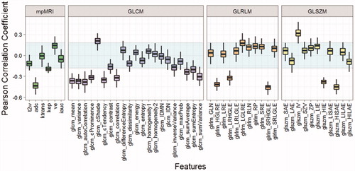
Results of Pearson’s correlations between individual feature and tumour grade are shown in Figure 1. The mpMRI parameters, ADC and k_ep were significantly correlated with tumour grade (–0.43, p < .01; –0.19, p = .04, respectively). V_e was moderately correlated with tumour grade but it was not statistically significant (0.15, p = .14). No significant correlations were found in T2w, K^trans and IAUC (p = .21, .89 and .56, respectively). In T2w, 10 GLCM-TFs had a significant correlation with tumour grade (p<.05). Six TFs based on GLRLM and GLSZM were also found to be significantly correlated with tumour grade (p<.05). Among all T2w TFs, 2 (SRHGLE and HISAE) had higher correlation coefficients than ADC, and SIHGLE had the largest absolute value of correlation coefficient (–0.46, p<.01).

Figure 1. Correlation between features and tumour grade (Y-axis: Pearson’s correlation coefficient). The statistically insignificant region is shown in the shaded region (p < .05).

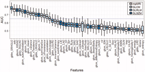
Each individual feature was used as a classifier (single-feature classifier) for tumour grade stratification and their performances were evaluated by AUC of the ROC curve (Figure 2). SRHGLE had the highest AUC (0.78, 95% CI [0.72–0.84]), which was followed by ADC (0.76, 95% CI [0.70–0.82]) and HISAE (0.76, 95% CI [0.70–0.81]).

Figure 2. Performances of single feature classifier for tumour grade stratification. Fifteen features have median AUC values above 0.65, indicated by the dashed line (Y-axis: area under the curve, AUC).

Study 2: horizontal comparison of four feature sets

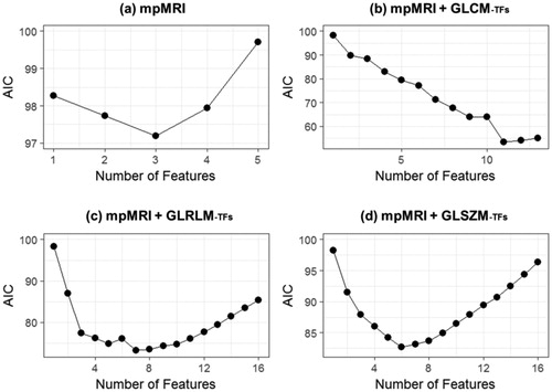
In the second study, feature selection was carried out within the four predefined feature sets, which included (1) mpMRI with no TFs (mpMRI alone), (2) mpMRI with GLCM-TFs, (3) mpMRI with GLRLM-TFs and (4) mpMRI with GLSZM-TFs. In four feature sets, a general pattern was found where the AIC first decreased and reached a minimum before it increased, with increasing numbers of features (Figure 3). The best feature subsets were selected based on minimum AIC (S8), indicating adding more features did not add to the predictive power.

Figure 3. Feature selection using AIC for four feature sets. The plots show the AIC values for a given number of features in feature selection. The feature subset with the lowest AIC was chosen for each group (AIC: Akaike’s information criterion).

Logistic regression models were trained using the selected features within each feature set and evaluated using AUC of the ROC curves. The highest performance was achieved in feature Set b (mpMRI + GLCM-TFs, AUC  =  0.84), followed by feature Set c (mpMRI + GLRLM-TFs, AUC  =  0.82) and feature Set d (mpMRI + GLSZM-TFs, AUC  =  0.78). Results of the feature selection can be found in S8. Feature Set a (mpMRI alone, AUC  =  0.69) had the lowest performance (Table 2). However, statistical significance of AUC was only found between Set b and Set a (p = .005).

Table 2. Performance evaluation of four feature sets using fivefold cross validation.

Feature set	AUC [95% CI]	p Value
mpMRI	0.69 [0.56, 0.82]	<.01
mpMRI + GLCM-TFs	0.84 [0.74, 0.95]	<.01
mpMRI + GLRLM-TFs	0.82 [0.69 0.95]	<.01
mpMRI + GLSZM-TFs	0.78 [0.72, 0.84]	<.01

mpMRI: multiparametric MRI; GLCM: grey-level co-occurrence matrix; GLRLM: grey-level run length matrix; GLSZM: grey-level size zone matrix; TF: texture features; AUC: area under the curve.

Study 3: combining all features

In the final study, seven features were selected from the original 49 features using the learning pipeline. The resulting model achieved an AUC of 0.91 (95% CI [0.87, 0.95]). Compared with the highest performing feature subset (mpMRI + GLCM-TFs) in Study 2, combining all features resulted in an increase in AUC of 0.07 on average. Statistical significance of AUC values was demonstrated with feature sets in Study 2 (p values: Set b, .05; Set c, .05; Set d, .0004).

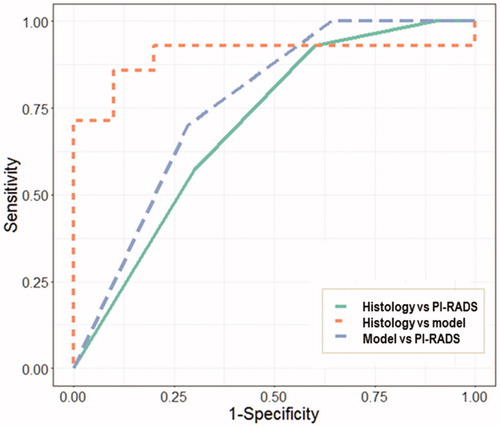
Using histology as the ground truth, the predictive model achieved a higher performance (AUC = 0.90) than the PI-RADS score (AUC = 0.70). A moderate level of agreement (AUC  =  0.86) was demonstrated between the predictive model and PI-RADS score (Figure 4).

Figure 4. The receiver operating characteristics curves for histology versus PI-RADS scores (AUC = 0.70), histology versus the model prediction (AUC = 0.90) and the model prediction versus PI-RADS scores (AUC = 0.86) (AUC: area under the curve).

Discussion

In this study, we presented a methodology to stratify prostate tumour grade. At the ROI-wise level, the final model achieved a promising AUC at 0.91 when different feature families were combined. The final model contained seven features which was comparable with the number of features in Study 2 (Figure 3(b–d)). Despite its significant improvement over other feature sets, the final model does not require additional computational effort to be applied. This also complied with the rules that for intermediately correlated features (S9 and S10), the feature number should be around $\sqrt{n}$ ($\sqrt{n}\approx 10$ in this study) [48].

While the motivation for this work was to define the spatial distribution of tumour cells defined by tumour grade for the purpose of biologically optimised radiotherapy, we also considered the reliability of the model, when used with the biopsy information, to accurately grade the disease for the purpose of treatment selection (S11). Here, we compared the highest grade reported (biopsy or model prediction) with the histology grade for each individual focus. These data are presented in S11 in 24 patients where biopsy, model prediction and histology data were complete. Of the 24 patients, 18 cases were consistently reported in the biopsy, model and histology. In two cases, the biopsy and model predicted LG in contract to histology which was reported as HG. In this case, the model performed no worse than the biopsy alone. In two cases, the model predicted LG, but the biopsy and histology reported HG. In this case, selection of treatment would not be compromised because the biopsy data would influence treatment decision. In one case, the model and histology reported HG but the biopsy LG. In this case, the model result would correctly influence treatment decision in contrast to the biopsy result which would have underestimated the disease. While these results suggest the model may be useful in the treatment making decision, further work is required to verify the model performance for this purpose.

To understand the relative value of each feature, a correlation analysis and single-feature performance analysis was performed (Figure 1). Hence, we chose the Pearson correlation coefficient to evaluate the association, rather than a between-group statistical test (e.g., a t-test for comparing the mean). Consistent with previous reports [13–15], ADC was found to have a significant correlation with tumour grade (p < .01) and outperformed all other mpMRI parameters (–0.43, p < .01; AUC = 0.76). It has previously been shown that ADC has a positive association with the percentage area of luminal space and negatively correlates with epithelium volume [22,49]. As the Gleason Grade increases, the tissue morphology changes from well-formed glands to poorly formed glands [1], which results in decreased luminal space. In addition, Lawrence et al. reported that the epithelium percentage increased significantly in GS ≥ 4 + 3 tumours compared with GS ≤ 3 + 4 tumours [50] which can also lower the ADC. Hence, this may explain the negative association between ADC and tumour aggressiveness.

When considering all TFs in isolation (Study 1), we found two high performing TFs (SRHGLE and HISAE from GLRLM and GLSZM, respectively) had comparable or greater AUC values than ADC (AUC values of 0.78, 0.76 and 0.76, respectively). While two temporal resolutions (3.62 s and 7.2 s) were used in DCE-MRI acquisition, this affected only the sampling rate rather than the shape of the pharmacokinetic curve and hence the resulting parametric maps were comparable. It is surprising that no pharmacokinetic parameters have previously been reported as significantly correlating with GS [21–24]. Chen et al. [20] reported that DCE-MRI washout gradient significantly correlated with GS, however, no correlation was found with quantitative pharmacokinetic parameters (K^trans, k_ep and V_e). In our study, K^trans and IAUC did not achieve a significant correlation (p = .89, .56, respectively), which agreed with Chen’s findings. This indicates that while K^trans and IAUC are sensitive in detecting differences between lesions and normal tissues [13,51], they do not discriminate between lesions with different GS. The remaining two pharmacokinetic parameters (k_ep and V_e) were moderately correlated with tumour grade. Due to the mathematical relationship between k_ep and V_e (k_ep = K^trans/V_e), the correlation coefficient between tumour grade and k_ep should have an opposite sign to that of V_e. This was reflected in our results as tumour grade was positively correlated with V_e (0.15) but negatively correlated with k_ep (–0.19). Similar trends were found in a previous study by Oto et al. [24] (V_e, r = 0.015; k_ep, r = –0.091) although their results were not significant (p = .906, p = .469, respectively). The potential value of V_e and k_ep requires further investigation and validation.

In multivariate analysis, collinearity and multicollinearity can lead to unstable models [52,53]. Haralick et al. commented that a high correlation can exist between TFs, and that feature selection should be carried out [54]. Hence, in the second study, we applied the feature selection method developed for regression models proposed by Sestelo et al., which was tested for different levels of correlation [44]. Examining collinearity after feature selection found correlation coefficients were mostly moderate (between –0.5 and 0.5, example of one model shown in S9 and S10). Following feature selection, we found group b (mpMRI with GLCM: T2w, ADC, V_e with eight GLCM-TFs) had the strongest performance (AUC  =  0.84) compared with the remaining feature sets. Hence, when compared with the highest performing single features (considered in isolation: SRHGLE, HISAE, ADC), we confirm that the power to differentiate HG and LG disease can be improved with the addition of GLCM features. This agrees with previous studies which utilised GLCM features [26–29]. In our study, the remaining feature sets did not outperform the single highest performing features. In the final study, we considered all features combined to judge the value of multiple select features compared with the single top performing features from Study 1 and the top performing subset from study 2. This combined model demonstrated superior performance (AUC  =  0.91) compared with feature set b (mpMRI with GLCM, AUC  =  0.84) and the highest performing single features (AUC  =  0.76–0.78).

We acknowledge the limitations in this study. First, the analysis did not separate the prostate by zones due to the small size of samples. As differences exist between the peripheral zone and the transition zone [55], modelling on the individual zones could increase performance [56]. Second, according to the registration framework, the average uncertainty in co-registration of the mpMRI data and the ground truth histology was 3.3 mm. This is based on a full 3D co-registration framework, and validation of the framework relied on matching features in T2w MRI and histology, hence we consider this a conservative estimate of uncertainty due to the difficulties in accurately identifying reliable corresponding features. Although average values of feature maps were used for each ROI, the influence of registration uncertainty could not be eliminated. Potentially improvements in validating registration accuracy may minimise this uncertainty.

The use of MR guided biopsies and focal approaches to treatment are rapidly becoming standard of care in many centres, though many of the technical challenges are yet to be addressed due to lack of high quality, quantitative data [4]. Our study used a moderately large sample size of 30 patients and 111 ROIs for analysis. In contrast to many other studies that have defined tumour regions on MRI, we used histology as ground truth labels with annotations generated by an experienced uro-pathologist (CM). These annotations were transposed to the mpMRI data using a sophisticated co-registration framework. Hence we have used a high quality dataset. Future studies will consider the generalisability of these conclusions across different MR scanners.

Conclusions

In this study, we considered the relative merit of individual signal intensities, parametric and pharmacokinetic parameters from mpMRI and TFs from T2w MRI. As in previous studies, we found mpMRI plus the TF set GLCM improved the predictive power of models designed to predict high and low grade disease compared with ADC alone. In addition, our study demonstrated that features selected from two additional families of TFs, when used in combination, improved the AUC value from 0.74 for ADC alone, and 0.84 for mpMRI plus GLCM, to 0.91 for the combined feature set. This study was motivated by the need to accurately define regions of HG disease for the purpose of personalised biologically optimised radiotherapy. While these findings require further validation in a larger multi-centre cohort, we suggest that incorporation of the additional TFs from T2w images may be of value for the purpose of defining aggressive tumour regions for dose escalation.

Acknowledgments

The authors would like to show gratitude to Courtney Savill and Lauren Caspersz for histology specimen preparation and MRI acquisition.

Disclosure statement

The authors do not have any conflict of interest to disclose.

Additional information

Funding

This study was supported by NHMRC [grant 1126955], PdCCRS [grant 628592] with the following funding partners: Prostate Cancer Foundation of Australia (PCFA), the Radiation Oncology Section of the Australian Government of Health and Aging and Cancer Australia. Yu Sun is funded by the Melbourne International Research Scholarship, the Movember Young Investigator Grant through PCFA and CTx Top-up Funding. Hayley Reynolds is funded by a Movember Young Investigator Grant awarded through PCFA’s Research Program.

References

- Gordetsky J, Epstein J. Grading of prostatic adenocarcinoma: current state and prognostic implications. Diagn Pathol. 2016;11:2–9.
- Evans MA, Millar JL, Earnest A, et al. Active surveillance of men with low risk prostate cancer: evidence from the Prostate Cancer Outcomes Registry-Victoria. Med J Aust. 2018;208:439–443.
- van der Poel HG, van den Bergh RCN, Briers E, et al. Focal therapy in primary localised prostate cancer: the European Association of Urology Position in 2018. Eur Urol. 2018;74:84–91.
- Haworth A, Williams S. Focal therapy for prostate cancer: the technical challenges. JCB. 2017;9:383–389.
- Bossart EL, Stoyanova R, Sandler K, et al. Feasibility and initial dosimetric findings for a randomized trial using dose-painted multiparametric magnetic resonance imaging-defined targets in prostate cancer. Int J Radiat Oncol. 2016;95:827–834.
- Lips IM, van der Heide UA, Haustermans K, et al. Single blind randomized phase III trial to investigate the benefit of a focal lesion ablative microboost in prostate cancer (FLAME-trial): study protocol for a randomized controlled trial. Trials. 2011;12:255.
- Haworth A, Williams S, Reynolds H, et al. Validation of a radiobiological model for low-dose-rate prostate boost focal therapy treatment planning. Brachytherapy. 2013;12:628–636.
- Hassanzadeh E, Glazer D, Dunne R, et al. Prostate imaging reporting and data system version 2 (PI-RADS v2): a pictorial review. Abdominal Radiology. 2017;42:278–279.
- Weinreb JC, Barentsz JO, Choyke PL, et al. PI-RADS prostate imaging – reporting and data system: 2015, version 2. Eur Urol. 2016;69:16–40.
- Barentsz JO, Richenberg J, Clements R, et al. ESUR prostate MR guidelines 2012. Eur Radiol. 2012;22:746–757.
- Penzkofer T, Tempany-Afdhal CM. Prostate cancer detection and diagnosis: the role of MR and its comparison with other diagnostic modalities – a radiologist’s perspective. NMR Biomed. 2014;27:3–15.
- Le BD. Apparent diffusion coefficient and beyond: what diffusion MR imaging can tell us about tissue structure. Radiology. 2013;268:318–322.
- Verma S, Turkbey B, Muradyan N, et al. Overview of dynamic contrast-enhanced MRI in prostate cancer diagnosis and management. AJR Am J Roentgenol. 2012;198:1277–1288.
- Verma S, Rajesh A, Morales H, et al. Assessment of aggressiveness of prostate cancer: correlation of apparent diffusion coefficient with histologic grade after radical prostatectomy. Am J Roentgenol. 2011;196:374–381.
- Woo S, Kim SY, Cho JY, et al. Preoperative evaluation of prostate cancer aggressiveness: using ADC and ADC ratio in determining Gleason score. Am J Roentgenol. 2016;207:114–120.
- Donati OF, Mazaheri Y, Afaq A, et al. Prostate cancer aggressiveness: assessment with whole-lesion histogram analysis of the apparent diffusion coefficient. Radiology. 2014;271:143–152.
- Giannini V, Vignati A, Mirasole S, et al. MR-T2-weighted signal intensity: a new imaging biomarker of prostate cancer aggressiveness. Comput Methods Biomech Biomed Eng Imaging Vis. 2016;4:130–134.
- Rosenkrantz AB, Kopec M, Kong X, et al. Prostate cancer vs. post-biopsy hemorrhage: diagnosis with T2- and diffusion-weighted imaging. J Magn Reson Imaging. 2010;31:1387–1394.
- Wang L, Mazaheri Y, Zhang J, et al. Assessment of biologic aggressiveness of prostate cancer: correlation of MR signal intensity with Gleason grade after radical prostatectomy. Radiology. 2008;246:168–176.
- Chen Y-J, Chu W-C, Pu Y-S, et al. Washout gradient in dynamic contrast-enhanced MRI is associated with tumor aggressiveness of prostate cancer. J Magn Reson Imaging. 2012;36:912–919.
- Isebaert S, Keyzer FD, Haustermans K, et al. Evaluation of semi-quantitative dynamic contrast-enhanced MRI parameters for prostate cancer in correlation to whole-mount histopathology. Eur J Radiol. 2012;81:e217–e222.
- Langer DL, van der Kwast TH, Evans AJ, et al. Prostate tissue composition and MR measurements: investigating the relationships between ADC, T2, Ktrans, ve, and corresponding histologic features. Radiology. 2010;255:485–494.
- Padhani AR, Gapinski CJ, Macvicar D. a, et al. Dynamic contrast enhanced MRI of prostate cancer: correlation with morphology and tumour stage, histological grade and PSA. Clin Radiol. 2000;55:99–109.
- Oto A, Yang C, Kayhan A, et al. Diffusion-weighted and dynamic contrast-enhanced MRI of prostate cancer: correlation of quantitative MR parameters with Gleason score and tumor angiogenesis. Am J Roentgenol. 2011;197:1382–1390.
- Yang F, Ford JC, Dogan N, et al. Magnetic resonance imaging (MRI)-based radiomics for prostate cancer radiotherapy. Transl Androl Urol. 2018;7:445–458.
- Rozenberg R, Thornhill RE, Flood TA, et al. Whole-tumor quantitative apparent diffusion coefficient histogram and texture analysis to predict Gleason score upgrading in intermediate-risk 3 + 4 = 7 prostate cancer. Am J Roentgenol. 2016;206:775–782.
- Nketiah G, Elschot M, Kim E, et al. T2-weighted MRI-derived textural features reflect prostate cancer aggressiveness: preliminary results. Eur Radiol. 2016;27:3050–3059.
- Fehr D, Veeraraghavan H, Wibmer A, et al. Automatic classification of prostate cancer Gleason scores from multiparametric magnetic resonance images. Proc Natl Acad Sci USA. 2015;112:6265–6273.
- Vignati A, Mazzetti S, Giannini V, et al. Texture features on T2-weighted magnetic resonance imaging: new potential biomarkers for prostate cancer aggressiveness. Phys Med Biol. 2015;60:2685–2701.
- Galloway MM. Texture analysis using gray level run lengths. Comput Graph Image Process. 1975;4:172–179.
- Thibault G, Fertil B, Navarro C, et al. Shape and texture indexes application to cell nuclei classification. Int J Patt Recogn Artif Intell. 2013;27:1357002.
- Reynolds HM, Williams S, Zhang A, et al. Development of a registration framework to validate MRI with histology for prostate focal therapy. Med Phys. 2015;42:7078–7089.
- Chan TY, Partin AW, Walsh PC, et al. Prognostic significance of Gleason score 3 + 4 versus Gleason score 4 + 3 tumor at radical prostatectomy. Urology. 2000;56:823–827.
- Lv D, Guo X, Wang X, et al. Computerized characterization of prostate cancer by fractal analysis in MR images. J Magn Reson Imaging. 2009;30:161–168.
- Viswanath SE, Bloch NB, Chappelow JC, et al. Central gland and peripheral zone prostate tumors have significantly different quantitative imaging signatures on 3 tesla endorectal, in vivo T2-weighted MR imagery. J Magn Reson Imaging. 2012;36:213–224.
- Viswanath S, Palumbo D, Chappelow J, et al. Empirical evaluation of bias field correction algorithms for computer-aided detection of prostate cancer on T2w MRI. Prog Biomed Opt Imaging - Proc SPIE. 2011;7963:79630V1–79630V12.
- Tustison NJ, Avants BB, Cook PA, et al. N4ITK: improved N3 bias correction. IEEE Trans Med Imaging. 2010;29:1310–1320.
- Cheadle C, Vawter MP, Freed WJ, et al. Analysis of microarray data using Z score transformation. J Mol Diagn. 2003;5:73–81.
- Artan Y, Haider MA, Langer DL, et al. Prostate cancer localization with multispectral MRI using cost-sensitive support vector machines and conditional random fields. IEEE Trans Image Process. 2010;19:2444–2455.
- Artan Y, Langer DL, Haider MA, et al. Prostate cancer segmentation with multispectral MRI using cost-sensitive conditional random fields. ISBI’09. 2009 Jun 28–Jul 1; Boston, Massachusetts, USA: IEEE International Symposium on Biomedical Imaging; 2009. p. 278–281.
- Ozer S, Haider MA, Langer DL, et al. Prostate cancer localization with multispectral MRI based on relevance vector machines. 2009 Jun 28–Jul 01; Boston, Massachusetts, USA: IEEE International Symposium on Biomedical Imaging; 2009. p. 73–76.
- Ozer S, Langer DL, Liu X, et al. Supervised and unsupervised methods for prostate cancer segmentation with multispectral MRI. Med Phys. 2010;37:1873–1883.
- Lemaître G, Martí R, Freixenet J, et al. Computer-aided detection and diagnosis for prostate cancer based on mono and multi-parametric MRI: a review. Comput Biol Med. 2015;60:8–31.
- Sestelo M, Villanueva NM, Meira-Machado L, et al. FWDselect: an R package for variable selection in regression models. RJ. 2016;8:132–148.
- Bozdogan H. Model selection and Akaike’s information criterion (AIC): the general theory and its analytical extensions. Psychometrika. 1987;52:345–370.
- Peng C-Y, Lee KL, Ingersoll GM. An introduction to logistic regression analysis and reporting. J Educ Res. 2002;96:3–14.
- Kumar R, Indrayan A. Receiver operating characteristic (ROC) curve for medical researchers. Indian Pediatr. 2011;48:277–287.
- Suh E, Dougherty ER, Lowey J, et al. Optimal number of features as a function of sample size for various classification rules. Bioinformatics. 2004;21:1509–1515.
- Chatterjee A, Watson G, Myint E, et al. Changes in epithelium, stroma, and lumen space correlate more strongly with Gleason pattern and are stronger predictors of prostate ADC changes than cellularity metrics. Radiology. 2015;277:751–762.
- Lawrence EM, Warren AY, Priest AN, et al. Evaluating prostate cancer using fractional tissue composition of radical prostatectomy specimens and pre-operative diffusional kurtosis magnetic resonance imaging. PLoS One. 2016;11:1–12.
- Khalifa F, Soliman A, El-Baz A, et al. Models and methods for analyzing DCE-MRI: a review. Med Phys. 2014; 41:124301.
- Kuhn M. Building predictive models in R using the caret package. J Stat Softw. 2008;28:1–26.
- Dormann CF, Elith J, Bacher S, et al. Collinearity: a review of methods to deal with it and a simulation study evaluating their performance. Ecography; 2013;36:27–46.
- Haralick RM, Shanmugam K, Dinstein I. Textural features for image classification. IEEE Trans Syst Man Cybern. 1973;3:610–621.
- Lee JJ, Thomas I-C, Nolley R, et al. Biologic differences between peripheral and transition zone prostate cancer. Prostate. 2015;75:183–190.
- Dikaios N, Alkalbani J, Abd-Alazeez M, et al. Zone-specific logistic regression models improve classification of prostate cancer on multi-parametric MRI. Eur Radiol. 2015;25:2727–2737.