Combining Gaussian processes, mutual information and a genetic algorithm for multi-target optimization of expensive-to-evaluate functions

Abstract

A novel approach to multi-target optimization of expensive-to-evaluate functions is explored that is based on a combined application of Gaussian processes, mutual information and a genetic algorithm. The aim of the approach is to find an approximation to the optimal solution (or the Pareto optimal solutions) within a small budget. The approach is shown to compare favourably with a surrogate based online evolutionary algorithm on two synthetic problems.

Keywords:

• multi-target optimization
• experimental design
• information gain
• hypervolume indicator

1. Introduction

In target optimization one is concerned not with finding the global optimum (unless the target happens to be one), but rather with finding solutions associated with desired values of the underlying process/es. Such optimization problems often arise in product design. In particular, when novel materials and/or methods are involved, it is usually required that certain desired specifications/properties of the product are adhered to. For example, in designing a formulated product such as facial cream (using a constantly updated set of ingredients) it is important that certain product properties are achieved, for example viscosity and transparency, amongst other characteristics. In general, this poses a challenging engineering problem in that accurate prediction of properties of formulated consumer products based on composition is difficult, due to the physical complexity of the system Peremezhney et al. (2012). Lack of knowledge about the underlying process leads to the need for an often large number of interactions with the real system. For some applications the number of interactions that can be performed is limited due to the high cost of the resources involved. In these instances an attractive strategy is to sequentially select experiments that are optimal both in terms of experimental design and in terms of identification of suitable solution/s. The strategy is usually implemented via the employment of a surrogate model for the approximation of values of the response variable in combination with a selective one-at-a-time sampling strategy where information from past experiments is used to determine the design of the next one. One of the most prominent algorithms for such sequential optimization is the Efficient Global Optimization (EGO) algorithm Jones, Schonlau, and Welch (1998). Since its introduction, the algorithm has been adapted for different types of optimization problem, including target optimization. In Wenzel et al. (2010), for instance, the concepts of desirability Harrington (1965) and virtual observations Cox and John (1997) are made use of to construct an algorithm capable of identifying and, with each iteration, improving on a cluster of solutions that best associate with target values. Even though the algorithm undoubtedly explores globally throughout the search, it is not designed to actively search actively for solutions that would allow one to gain the most information about the underlying process (i.e. solutions optimal in terms of experimental design). In this article a novel approach to sequential multi-target optimization is proposed that explicitly incorporates maximization of information gain as one of its objectives.

Let ; , where d is the dimension of the problem and Ω the decision space, be the vector of values of the input variables, scalars and y* the corresponding observation obtained via interacting with the real system and a target, and the set of candidate solutions (obtained via discretization of the decision space). Then, for a single-target optimization, the objective is to minimize the sum of regrets

where i is the iteration number and is used to mean absolute value or norm one. Or, in other words, to find

in as few iterations as possible. Note that the situation where there are multiple solutions to (2) may arise. It is assumed that this scenario would be handled by the end user, ranking the solutions further by applying relevant cost functions. For instance, if the solutions are compositions of ingredients in a formulation, then they can be further ranked in terms of the cost of ingredients, or the proportion of a particular ingredient, etc.

The procedure for sequential single-target optimization in an expensive-to-evaluate function scenario could be as follows

1. Construct a cheap-to-evaluate surrogate model and train it on a sample of points , h≪n (the training set).

2. Using the surrogate model's predictions, select that

   • maximizes information gain about the underlying process – exploration;

   • minimizes predicted regret, i.e. satisfies (2) – exploitation.

3. Evaluate via interacting with the real system and obtain .

4. Include the pair in the training set and update the model.

5. Iterate until there is no improvement on the current optimum or the available budget has expired.

The above procedure requires that, at each iteration, two objectives are optimized simultaneously. One way to go about it is to search for a set of non-dominated solutions – the Pareto set (where a solution is non-dominated if it cannot be superseded by another solution that improves an objective without worsening another one). A good way to select just one from a Pareto set is to choose a solution with the highest value of hypervolume indicator Zitzler and Thiele (1998). The hypervolume indicator is the volume of the fitness space that is dominated by a solution and is bounded by a reference point (see Figure 1). Also, the procedure entails choosing from a predetermined decision set. Although practical in terms of computational speed, this is limiting in terms of accuracy. It would, hence, be beneficial to find a compromise between the increase in the level of discretization and the search of the entire decision space. The proposed compromise is first to identify a set of non-dominated solutions from a discrete set of candidate solutions, then to search in the neighbourhood of these solutions, using a real-coded genetic algorithm – non-dominated sorting genetic algorithm II (NSGA-II) Deb et al. (2002) is employed – for a solution with the highest value of hypervolume indicator.

Figure 1. Hypervolume (shaded area), bounded by a reference point R, of a three point Pareto set . The hypervolume of point P2 is the area of the rectangle whose diagonally opposite corners are P2 and R.

Industrial target optimization problems, however, often involve more than one target. For instance, a formulator may need to optimize a formulation for a particular value of viscosity and opacity. The procedure described above can be extended to a multi-target case by constructing a separate surrogate model for each underlying process and for , replacing the values of information gain and regret associated with it with suitable aggregates. After the termination of the multi-target optimization, all of the non-dominated solutions (in relation to the actual targets) could be identified and presented to the end user for further consideration.

For the surrogate model, Gaussian processes, as they provide a principled way of assessing uncertainty of the model, have successfully been used in many optimization problems and are the choice for the approach discussed here. As has already been mentioned, the sampling criterion is required to account for the need to exploit the knowledge acquired so far as well as to gain more knowledge about the underlying processes. The former can be achieved by choosing that, according to surrogate model's prediction, is closest to the target; the latter can be achieved by choosing that is predicted to reduce the uncertainty about the rest of the input space the most, which can be interpreted as the greatest increase in mutual information Guestrin, Krause, and Singh (2005) between and the rest of the input space. Gaussian processes allow one to deal efficiently with both demands on the sampling criterion.

The approach proposed in this article is compared with a surrogate based online evolutionary algorithm El-Beltagy and Keane (2001) that also uses Gaussian processes. It should be noted that other surrogate based online evolutionary algorithms exist that are similar in their approach – see, for instance, Emmerich, Giannakoglou, and Naujoks (2006) and Liu, Zhang, and Gielen (2013). The attractive features of these algorithms are: (1) they have an evolutionary algorithm at the core, capable of solving multi-dimensional multi-modal problems; and (2) they attempt to strike a balance between the need to reduce the amount of expensive evaluations and the need to improve on the quality of the surrogate model. Although both the approach presented in this work and the algorithm it is compared with use Gaussian processes, their application is different, which makes for an interesting comparison. In the rest of the article, the proposed algorithm is referred to as the Multi-Objective Active Learner (MOAL) algorithm and the abbreviation SOEA is used for the Surrogate based Online Evolutionary Algorithm.

The article is organized as follows: in Section 2, Gaussian processes and ‘mutual information’ are briefly introduced, followed by a description of the MOAL algorithm in Section 3; in Sections 4 and 5, synthetic examples of the application of the MOAL and SOEA algorithms are presented; results are discussed in Section 6, and conclusions are drawn in Section 7.

2. Methods

2.1. Gaussian processes

The assumption is that the observations associated with the inputs to the system have a (multivariate) Gaussian joint distribution. Here, a random variable is an observation associated with a particular input. For any subset of the random variables, their joint distribution will also be Gaussian. A Gaussian Process (GP) is a generalization of multivariate Gaussians to an infinite number of random variables. According to a GP definition, the joint distribution over observations associated with every finite subset of inputs is Gaussian. These joint distributions are defined by a GP through the use of a mean function, m(·), and a covariance function, . For an observation associated with input , its mean is given by and for a pair of observations and their covariance, , is given by . A common choice is to apply a Gaussian process with zero mean function and Automatic Relevance Determination (ARD) squared exponential covariance function

In the above, is the signal variance and l_d is an individual characteristic length scale for each input dimension x_d. However, it is sensible to assume measurement noise to be present. Hence, each observation can be thought of as related to an underlying process through a Gaussian noise model:

where are Independent Identically Distributed (IID) random errors. And so the final expression for the covariance function – the prior on the noisy observations – can be written as

where is the Kronecker delta function. forms a set of hyperparameters of the covariance function. To incorporate the knowledge that the training data provides about the process, the joint distribution of the observed target values and function values at test locations under the prior is written and then conditioned on the observations. The necessary Gaussian identities employed are where and are jointly Gaussian random vectors, and the marginal distribution of together with the conditional distribution of given

So now, given a number of inputs X, corresponding observations , and an unobserved input , for ,

And the conditional probability, , follows a Gaussian distribution: The mean and variance of this distribution is used to compute the best estimate and the uncertainty of :

A number of models can be constructed depending on the choice of the values of the hyperparameters of the covariance function. Figure 2 illustrates two output vectors where the mean and variance of each output has been computed using (7) and (8), but where the values of the hyperparameters of the covariance function are different. To choose the best model for the data available, a search is carried out for the values of the hyperparameters that maximize the marginal likelihood – the probability of the data given the hyperparameters, where n is the number of training examples. To set the hyperparameters, partial derivatives of the marginal likelihood w.r.t. the hyperparameters are obtained and used in conjunction with a gradient based optimizer. To train a GP model, a choice has to be made (utilizing prior knowledge) between different functional forms for the mean and covariance functions as well as the adaptation of the hyperparameters of these functions. In the absence of prior knowledge, a variety of functional forms could be investigated via the comparison of marginal likelihoods – for more details see Rasmussen and Williams (2006). In this work, only GPs with zero mean function, a squared exponential (ARD) covariance function, and GPs with zero mean function and Matérn_(ν=3/2) covariance function are considered.

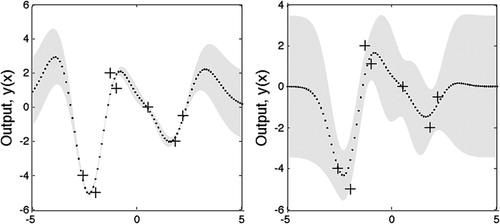
Figure 2. Two output vectors where the mean and variance of each output has been computed using (7) and (8), but where the values of the hyperparameters of the covariance function are different. The training data are shown by ‘+’ signs. The output predictions (dots) were generated using a GP with the covariance function as in (5) with: left – (l, σ_f, σ_n) = (1, 1, 0.1); right – (l, σ_f, σ_n)=(√3, 0.5, 0.8). Both plots also show the two standard-deviation error bars for the predictions obtained using these values of the hyperparameters.

2.2. Mutual information

The Mutual Information (MI) of two discrete random variables X and Y measures how much knowing one of these variables reduces uncertainty about the other. It is expressed as

where is a marginal entropy – the amount of uncertainty about random variable X and is a conditional entropy – the amount of uncertainty remaining about X after Y is known – computed as

The entropy of a Gaussian random variable X conditioned on variable Y is a monotonic function of its variance:

If X is assumed to be an observation associated with a particular input to the system as discussed in the previous section, for instance, then, using GP regression, the predicted value of is easily computed using (8). Also, as the computation in (8) only depends on the inputs, it is possible to compute H(X|Y) before the actual observation is made. It is useful, in the context of optimization, to think of a discretized input space as a set of random variables. Let X_L be such a set of random variables, X_T be any subset of X_L and x any random variable in , then the mutual information , expressed as is the information gain, or the amount of uncertainty remaining about (the rest of the input space), if x is revealed.

3. The MOAL algorithm

Consider n objectives, associated with n targets, as in (2), and a budget of t evaluations. Two sets of points are involved: (1) the training set X_T, which is used to train the surrogate models and which gains a point with each iteration of the algorithm; and (2) a set X_L of other solutions from a discretized decision space. A surrogate model is trained for each process. Then, at each iteration of the algorithm, the following steps are performed.

1. Using the surrogate models, estimates and the associated predicted variances of observations for each point , , are computed.

2. In relation to i’s objective, every point is referenced in two ways:

   1. the increase in mutual information it would provide (Guestrin, Krause, and Singh 2005):

      where (9), (10) and (11) were employed and Equation (8) is used to compute and ;

   2. the predicted value of regret

      where and y*⁽ⁱ⁾ are the predicted value of the response variable i at and the target value of the response variable i, respectively.

3. The sets and are mapped onto interval [0, 1]. The information about every point is first summarized as

   then the magnitudes and are computed. The following procedure¹ is then used to choose one point for sampling.

   1. All of the points are sorted according to non-domination, using the magnitudes and , and a Pareto set χ is identified. The point satisfying

      is chosen as the ‘current best’. Set χ is first reduced to size (to include only and at most z−1 ‘next best’ non-dominated points selected according to Equation 15) and then used as the first population for an NSGA-II algorithm (without crossover) to conduct a search for the maximizer.

   2. The NSGA-II algorithm is iterated M times. At each iteration:

      • following sorting and selection steps, mutations are carried out (by performing small perturbations of the input vectors) to obtain a set (of size ) of new points within the decision space;

      • each of the new points is referenced using (12) and (13) and one point is chosen according to (15). If the value computed for it using (15) is higher than that of the ‘current best’ point, it becomes the ‘current best’ point;

      • the ‘current best’ point after the last iteration is chosen for evaluation.

4. The evaluated point is added to the training set and the hyperparameters of the surrogate models are reoptimized.

Intuitively, the marginal increase in mutual information (Equation 12) decreases for points that are near the one that was just sampled, which means that the area will not be sampled again for a number of iterations. This has a direct affect on the accuracy of the algorithm. To overcome this problem, the decision set X_L can be re-sampled with density (where is the matrix of solutions collected so far), when, for instance, there has been no improvement in the value of the hypervolume indicator of the Pareto set for a number of iterations. Re-sampling with can be done using a mixture of Gaussians (with n components) as a density estimator, for instance. The value of the hypervolume indicator of the Pareto set is obtained as follows: first, the observations , collected so far, are transformed as

where

then, from the transformed observations, the non-dominated set is identified and the value of hypervolume indicator (for the whole of the non-dominated set), bounded by a reference point [1, 1], is computed.

The algorithm stops once the budget of evaluations is exhausted. The final Pareto set is presented to the end user. For comparison of performance against other algorithms (or against optimum performance, if such information is available), the value of the hypervolume indicator for the final Pareto set (bounded by a reference point [1, 1]) can also be computed. To reduce computational complexity, is calculated using only k points, where

Namely, points are arranged in decreasing order according to their respective values of covariance with (computed using Equation 5) and the first k are selected.

4. Illustration of the approach

To illustrate the potential use of the approach, it is applied to simulate two multi-target optimization problems. The first problem illustrates the application of the algorithm to a two-target unconstrained optimization problem in which: (1) the two fictitious physical processes are simulated by the Ackley and the Booth functions (see Figure 3);

where

where (2) the number of design variables is two, with each one ranging from −30 to 30; and (3) both targets are global minima. Thus, the target vector is . The set of candidate solutions X_L comprises 1200 uniformly spread out over the decision space input vectors. The initial training set X_T comprises 16 input vectors, obtained as a Latin Hyper Cube (LHC) sample, and the corresponding values of two processes. The values of the Booth function are log transformed prior to regression. For this problem, a GP with zero mean and the Matérn covariance function were employed:

with positive parameters ν, and l, where K_ν is a modified Bessel function and ; ν=3/2 was chosen for this problem, for which (21) can be simplified Abramowitz and Stegun (1965) to

Parameters and l in (21) and (22) play the same role as in (3).

Figure 3. The Ackley function (a) and the Booth function (b) in two dimensions.

The first problem is challenging as, in order to approximate the optimal Pareto set well, the algorithm is required to find solutions that are near both global minima. A big proportion of the landscape of the Ackley function is featureless, thus a surrogate model trained on a small initial training set may not be able to produce satisfactory predictions for points in the target area, and the algorithm will be required to explore efficiently (i.e. to update the surrogate model with the most informative points quickly), for an optimization to converge on a satisfactory set of solutions within a small budget of evaluations. For the Booth function, the global optimum is inside a long, flat valley. To find the valley is not difficult; however, convergence to the global optimum is challenging. For the Ackley function, the global optimum is inside a narrow funnel, making it also non-trivial to locate.

The second problem illustrates the application of the algorithm to a two-target constrained optimization problem in which: (1) the two fictitious physical processes are simulated by the Levy and the Dixon & Price functions:

where

and (2) there are four design variables and one constraint. A constraint often encountered in industrial applications is applied:

where and T is user defined (T=10 is used for this problem). The situation is often encountered in experiments with formulated products, for instance where x_i are volumes of ingredients and T is the total volume per formulation.

Three random target vectors were chosen from the box . The set of feasible solutions X_L comprises 2000 uniformly spread out input vectors satisfying (25). The initial training set X_T comprises 30 uniformly spread out feasible input vectors and the corresponding values of two processes. Function values of both processes are log transformed prior to regression. For this problem, a GP with zero mean and squared exponential (ARD) covariance function was employed.

For both problems:

• process values are perturbed by noise drawn from ;

• in (18), k=2|X_T| is used;

• the NSGA-II algorithm is iterated 100 times per iteration of the main algorithm with a population size at most 1% of . For each mutation, the value of perturbation is drawn from the uniform distribution on the interval (0,α 60 and (0,α 10] for the first and second problems, respectively. Values of the parameter α from the interval [0.01, 0.1] were tested and α=0.01 selected;

• the decision set is re-sampled if there has been no improvement in the value of the hypervolume indicator for three consecutive iterations. To re-sample, only the solutions so far collected, , are considered. are assumed to belong to a mixture of Gaussian distributions with the number of components being that of the dimension of the input space. A Gaussian mixture model is fitted McLachlan and Peel (2000) and the parameter estimates (the components’ means, covariances and mixture proportions) are obtained using an Expectation Maximization (EM) algorithm. A set of random input vectors (of the same cardinality as X_L) is then drawn from the resulting distribution.

The hyperparameters² of surrogate models are fitted by optimizing the marginal likelihood using a conjugate gradient optimizer. To avoid bad local minima, five random restarts are tried, picking the run with the best marginal likelihood. Leave-one-out cross-validation is used to validate the models. Namely, for each point in the training set, its predicted function value along with the variance of the predicted value are computed using the rest of the set. Following Jones, Schonlau, and Welch (1998), cross-validated standardized residuals S_r are computed:

and a check is carried out that the standardized residuals are all in the interval [−3,+3]. The optimizations are run for 30 iterations. The observations thus collected are transformed using (16). From the transformed observations, the non-dominated set is identified and the value of the hypervolume indicator for the whole of the set (bounded by a reference point [1, 1]) is computed. The value is then compared against the one computed for the SOEA algorithm and the optimum or a suitably chosen baseline. In this work, a baseline is obtained by computing the value of the hypervolume indicator for non-dominated observations obtained having evaluated 10,000 uniformly spread out input vectors.

5. Brief description of the SOEA algorithm for multi-target optimization

In this work the approach proposed by El-Beltagy and Keane (2001) is adapted. The SOEA algorithm proceeds as follows.

• (1) An initial population of solutions of size N is chosen. The initial population of solutions and the corresponding observations are used as a training set to train surrogate models.

• (2) A GP with zero mean and squared exponential (ARD) covariance function is used. The setting up of the surrogate models, the validation and the hyperparameter optimization are as described in Section 4.

• (3) Using a multi-objective evolutionary algorithm (NSGA-II), the next population of solutions is obtained.

• (4) The trained surrogate models are used to predict the mean values and the corresponding variances of process values (see Equations 7 and 8) for each of the solutions obtained. From the predicted variances of the process values, the corresponding standard deviations are computed and normalized to be in the interval .

• (5) Solutions for which the normalized standard deviation of each predicted process value is below the currently allowable tolerance, , are assigned the predicted process values. For the rest, the values are established through interaction with the real system. These points are added to the training set. The value of is updated after each iteration of the overall algorithm. It is reduced as follows:

  where is the maximum allowable tolerance (initialized prior to optimization), t is the maximum number of interactions with the real system that are budgeted for, is the total number of solutions (up to the iteration i−1) that were evaluated via interacting with the real system, and N is the number of solutions in a population. Prior to the first iteration, is equal to . To avoid the infinite loop scenario, where evaluations are carried out using the surrogate models only, is reduced by half if, at iteration i, all of the solutions in the population have been assigned their predicted values.

• (6) The hyperparamteters of the surrogate models are reoptimized after each iteration. The overall algorithm is iterated until the budget is exhausted.

Once the budget of evaluations has been exhausted, the algorithm is stopped. The corresponding observations are transformed using (16). From the transformed observations, the non-dominated set is identified and the value of the hypervolume (using ([1, 1] as a reference point) is computed. The same decision set and the initial training set as for the MOAL algorithm are used. The initial value of the parameter is established through experimentation. Values between 0.05 and 0.5 are tested and a value of 0.1 selected.

6. Results and discussion

The MOAL and SOEA algorithms were tested on the problems presented in Section 4. Ten optimization runs were performed for each target vector and the mean values of the hypervolume indicator of the Pareto set, along with the corresponding standard deviations, were recorded (see Tables 1 and 2). These values were used to compare the performance of the algorithms. For both algorithms, the R⁽ⁱ⁾ in (16) were computed using observations from 10,000 uniformly spread out solutions. In real applications, these values would be established using all available observations after the last iteration of the algorithm.

Table 1.  Mean and standard deviation of the hypervolume indicator of the Pareto set for the target vector in problem 1 (after 10 runs of the algorithms).

MOAL	SOEA	Baseline
49.43%(4.11)	27.55%(15.86)	64.66%

Table 2.  Mean and standard deviation of the hypervolume indicator of the Pareto set for the target vectors in problem 2 (after 10 runs of the algorithms).

	MOAL	SOEA	Optimum/Baseline
Target vector 1	98.44%(0.68)	91.71%(3.90)	100%
Target vector 2	87.01%(3.31)	81.98%(4.00)	93.12%
Target vector 3	97.92%(0.50)	91.84%(1.78)	100%

As can be seen from the results, the MOAL algorithm performed better than the SOEA algorithm on both problems. The plausible explanation is that the MOAL algorithm is able to improve actively on the prediction quality of the surrogate models over the target area, and to do so rapidly (see Figure 4). Locating the areas of the decision space least well covered by the training set, whilst at the same time ‘promising’ in terms of gaining on the targets, allows the MOAL algorithm efficiently to discover the relevant [for the optimization] features of the underlying function landscape. By contrast, the SOEA algorithm is only concerned with reducing uncertainty in the search areas. In a situation where the underlying function landscape is challenging and the budget of evaluations is small, the algorithm can be very successful or unsuccessful depending on how quickly the evolutionary part of it can converge on solutions near the target area/s. This is reflected in the high value of the standard deviation of the hypervolume indicator for problem 1 (see Table 1).

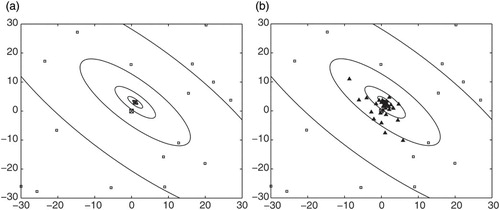
Figure 4. Contour plot of the Booth function with: (a) input locations of the initial training set, and (b) solutions obtained using the MOAL algorithm for an optimization run of 30 evaluations. Empty squares – solutions from the initial training set; filled triangles – solutions chosen by the MOAL algorithm; squares with a cross inside – the global minima of the Booth and the Ackley functions.

The following performance criteria can be used to assess the quality of the predictions of surrogate models.

• (1) The Standardized Mean Squared Error (SMSE) loss, which is the Mean Squared Error (MSE) normalized by the variance of the targets of the test cases (MSE on its own is sensitive to the overall scale of the target values).

• (2) The Negative Log Probability (NLP) of the target under the model,

  where and are the estimated mean and variance of the predictive distribution, respectively. This can be summarized by the Mean Negative Log Probability (MNLP), by averaging over the test set. This loss can be standardized by computing it relative to the NLP of a predictive model that ignores the inputs and always predicts using a Gaussian with the mean and variance of the training data. The MNLP will then be approximately zero for a simple predictive model and negative for a better one. The prediction quality of the surrogate models approximating the Booth function (as in problem 1) is used as an example (see Figure 5). The test set is chosen to be the solutions in and around the target area (a box).

Figure 5. Average SMSE values (a) and average MNLP values (b) computed for surrogate models approximating the Booth function in problem 1. The averages were computed over 10 optimization runs for budget sizes from 5 to 30 evaluations in increments of 5. Zero evaluations corresponds to the values computed for the model constructed using the initial training set.

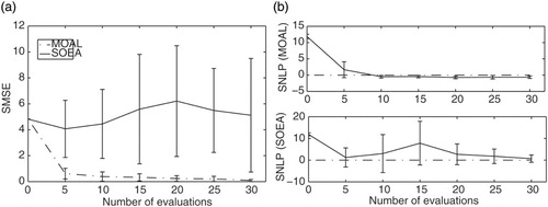
As can be seen from Figure 5, the surrogate models employed to approximate the Booth function during optimization runs of the MOAL algorithm produced predictions with on average smaller errors (see the SMSE plot). There is a big drop in the value of SMSE after just five evaluations, and a steady decrease thereafter, which indicates that the target area was found quickly, and that solutions are being chosen from it (the target area). The MNLP value also decreases rapidly by five evaluations, although the improvement is less pronounced thereafter. It can be argued that, for the SOEA algorithm, on average 30 evaluations were not enough to narrow down the search and hence adequately update its surrogate models.

The overall complexity of the MOAL algorithm is mostly due to the computation of the inverse of the covariance matrix (using Cholesky decomposition) for obtaining conditional entropies and using (11) in Section 2. The computational complexity for the approximation of the conditional entropies are and for and , respectively, where (the number of points in the decision space, as per discretization, plus the additional points obtained through the application of the genetic algorithm) and t is the budget (number of evaluations). The increase in complexity comes with an increase in the number of evaluations and an increase in the discretization of the input space, where the latter is dependent on the dimensionality of the problem. With this in mind, it is thought that the MOAL algorithm is most suited for problems where the cost of the resources outweighs the computational burden. For instance, a formulator may need to optimize a formulation and have a very limited number of experiments to conduct, duo to the high cost of a particular ingredient. Or, in chemical reaction optimization, a particular process may require a long time to run its course.

7. Summary and conclusions

In this article a novel approach to multi-target optimization of expensive-to-evaluate functions based on the combined application of Gaussian processes, mutual information and NSGA-II was proposed. To illustrate the potential use of the approach, it was applied to simulate the optimization of target values of fictitious physical processes. Constrained and unconstrained optimization, using the proposed algorithm, was illustrated. The algorithm was compared against a surrogate based online evolutionary algorithm specifically designed for the optimization of expensive-to-evaluate functions. Results indicate that, using the hypervolume indicator as performance criteria, the proposed approach compares favourably against the surrogate based online evolutionary algorithm on tasks involving a small budget of evaluations. Although the computational complexity of the proposed algorithm is high, it is not foreseen to be a hindrance for the type of applications it is designed for. The authors appreciate that, at the time of writing the article, the performance of the proposed algorithm has not yet been tested on a large number and a variety of multi-target optimization problems. The proposed algorithm is intended to be employed in experimentation with formulated products in the near future.

Funding

Nicolai Peremezhney is grateful for a PhD scholarship from the University of Warwick Complexity Doctoral Training Centre; the Engineering and Physical Sciences Research Council (EPSRC).

Notes

1. Note that other techniques, alternative to the genetic algorithm (the ‘branch-and-bound’ algorithm, for instance) could be used to find a solution to the single objective, constrained (by the boundaries of the decision space) optimization problem posed in (15).

2. The Gaussian Process Regression and Classification Toolbox version 3.1 for MATLAB™ by Carl Edward Rasmussen and Hannes Nickisch, downloaded from http://gaussianprocess.org/gpml/code was used.

References

- Abramowitz, M., and I. A. Stegun. 1965. Handbook of Mathematical Functions, 84–85. New York: Dover.
- Cox, D., and S. John. 1997. “A Statistical Method for Global Optimization.” In Multidisciplinary Design Optimization: State of the Art, edited by N. Alexandrow and M. Hussaini, 315–329. Philadelphia, PA: SIAM.
- Deb, K., A. Pratap, S. Agarwal, and T. Meyarivan. 2002. “A Fast and Elitist Multiobjective Genetic Algorithm: NSGA-II.” IEEE Transactions on Evolutionary Computation 6 (2): 182–197. doi: 10.1109/4235.996017
- El-Beltagy, M. A., and A. J. Keane. 2001. “Evolutionary Optimization for Computationally Expensive Problems Using Gaussian Processes.” In Proceedings of the International Conference on Artificial Intelligence, 708–714.: CSREA Press.
- Emmerich, M., K. Giannakoglou, and B. Naujoks. 2006. “Single and Multiobjective Evolutionary Optimization Assisted by Gaussian Rrandom Field Metamodels.” IEEE Transactions on Evolutionary Computation 10 (4): 421–439. doi: 10.1109/TEVC.2005.859463
- Guestrin, C., A. Krause, and A. Singh. 2005. “Near-Optimal Sensor Placements in Gaussian Processes.” In International Conference on Machine Learning (ICML), Bonn, Germany, August 7–11.
- Harrington, J. 1965. “The Desirability Function.” Industrial Quality Control 21 (10): 494–498.
- Jones, D., M. Schonlau, and W. Welch. 1998. “Efficient Global Optimization of Expensive Black-Box Functions.” Journal of Global Optimization 13 (4): 455–492. doi: 10.1023/A:1008306431147
- Liu, B., Q. Zhang, and G. Gielen. 2013. “A Gaussian Process Surrogate Model Assisted Evolutionary Algorithm for Medium Scale Expensive Optimization Problems.” IEEE Transactions on Evolutionary Computation, PP (99). doi: 10.1109/TEVC.2013.2248012.
- McLachlan, G., and D. Peel. 2000. Finite Mixture Models. Hoboken, NJ: Wiley.
- Peremezhney, N., C. Connaughton, G. Unali, E. Hines, and A. A. Lapkin. 2012. “Application of Dimensionality Reduction to Visualisation of High-Throughput Data and Building of a Classification Model in Formulated Consumer Product Design.” Chemical Engineering Research and Design 90 (12): 2179–2185. doi: 10.1016/j.cherd.2012.05.010
- Rasmussen, C. E., and C. K. I. Williams. 2006. Gaussian Processes for Machine Learning. Cambridge, MA: MIT Press.
- Wenzel, S., S. Straatmann, L. Kwiatkowski, P. Schmelzer, and J. Kunert. 2010. “A Novel Multi-Objective Target Value Optimization Approach.” In Classification as a Tool for Research: Studies in Classification, Data Analysis, and Knowledge Organization, edited by H. Locarek-Junge and C. Weihs, 801–809, Berlin: Springer-Verlag.
- Zitzler, E., and L. Thiele. 1998. “Multiobjective Optimization Using Evolutionary Algorithms – A Comparative Case Study.” In Parallel Problem Solving From Nature, V, edited by A. E. Eiben, T. Bäck, M. Schoenauer, and H. P. Schwefel, 292–301. Berlin: Springer-Verlag.