Comparison of model order reduction methods for optimal sensor placement for thermo-elastic models^*

* An abridged version of the manuscript was submitted to the CIRP sponsored conference on Conference on Thermal Issues in Machine Tools, 2018.

ABSTRACT

In this article an optimal sensor placement problem for a thermo-elastic solid body model is considered. Temperature sensors are placed in a near-optimal way so that their measurements allow an accurate prediction of the thermally induced displacement of a point of interest (POI). Low-dimensional approximations of the transient thermal field are used which allows for efficient calculations. Four model order reduction (MOR) methods are applied and subsequently compared with respect to the accuracy of the estimated POI displacement and the location of the sensors obtained.

KEYWORDS:

• Thermo-elastic model
• optimal sensor placement
• model order reduction

1. Introduction

This article is concerned with an optimal sensor placement problem for thermo-elastic solid body models. The goal is to place temperature sensors in a near-optimal way so that their measurements allow an accurate prediction of the thermally induced deformation at a particular point of interest (POI) in real time. The main motivation and example used throughout the article is the prediction of the deflection of the tool centre point (TCP) of a machine tool under thermal loading.

Sensor placement problems for partial differential equations (PDEs) are difficult optimization problems due to their large scale, as well as the intricate structure of the objective, which normally involves the estimator covariance matrix of the quantity estimated, or its asymptotic inverse, the Fisher information matrix. The present approach exploits the particular structure of thermo-elastic models. While the evolution of the temperature, T, is relatively slow, the deformation, $\mathit{u}$, is instantaneous. Moreover, mechanically induced heat sources are neglected, so that the coupling is $T\mapsto \mathit{u}$ is uni-directional.

In the optimal sensor placement problem, the objective is to choose sensor locations in such a way that the measurements contain the maximum amount of information with regard to the subsequent prediction of the thermally induced displacement at a POI, as opposed to the reconstruction of the temperature field itself. In order to reduce the complexity of the placement problem, model order reduction (MOR) for the temperature field is applied. In this article four model order reduction techniques are compared, namely proper orthogonal decomposition (POD), balanced truncation (BT), and two different moment matching (MM) approaches. The focus of this article is the application of modern model order reduction methods to the sensor placement procedure. Furthermore, the results of the sensor placement for these different MOR methods for the underlying temperature dynamics are compared.

To put this work into perspective, model order reduction techniques are frequently used in sensor placement problems involving PDEs, e.g. reaction–diffusion or convection–diffusion problems (Alonso, Frouzakis, and Kevrikidis 2004; Alonso et al. 2004; Armaou and Demetriou 2006; Green 2006; García et al. 2007) as well as fluid dynamics applications (Mokhasi and Rempfer 2004; Cohen, Siegel, and McLaughlin 2006; Willcox 2006; Yildirim, Chryssostomidis, and Karniadakis 2009), where POD is often the method of choice. In another class of applications involving mechanical deformation of large structures (Kammer 1991; Yi, Li, and Gu 2011; Meo and Zumpano 2005; Sun and Büyüköztürk 2015), modal analysis is employed as a reduction technique.

The references above fall into three categories concerning the actual placement strategy: forward, backward and simultaneous placement procedures. In the forward sequential setting, which is adopted in this article, sensors are placed one by one such that a maximal gain of information is obtained for each sensor. In the backward approach, a full set of possible sensor locations is chosen and those contributing the least amount of information are removed in a sequential fashion. Both are greedy algorithms. Simultaneous placement procedures can only be used, due to the combinatorial complexity, when the number of potential locations is relatively small.

The goal in all of the above references is to reconstruct the respective field of the underlying PDE from a limited number of measurements. In the setting under consideration, this would correspond to recovering the entire temperature field from a number of temperature measurements. By contrast, the objective in this article is to predict the mechanical displacement induced by that temperature field. This approach changes the metric with respect to which the gain of information is measured; see Körkel et al. (2008), Koevoets et al. (2007), and Herzog and Riedel (2015). In Koevoets et al. (2007), thermally induced displacements are estimated using temperature measurements as well. However, in contrast to the present work, only a small number of potential sensor locations is considered, and modal analysis is used. In Herzog and Riedel (2015), a sensor placement approach based on POD was presented. One drawback of this simulation based MOR technique is its dependence on the thermal load cycle used to obtain the snapshots. The present article is an extension of this work in which four different MOR techniques are compared, three of which do not depend on simulations and are thus more widely applicable.

The article is organized as follows. In the remainder of this section the thermo-elastic model is stated. The sequential placement strategy is described in detail in Section 3. The model order reduction techniques under consideration are presented in Section 4. Numerous numerical experiments are provided in Section 5, which allows a comparison of the MOR techniques in the context of sensor placement problems.

2. Thermo-elastic forward model

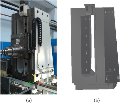
Before the sensor placement and model order reduction procedures are described, the model problem to be considered is introduced. The solid body whose thermo-mechanical displacement is to be considered will be denoted by Ω, and its surface by Γ. In the application at hand, Ω is the column of a machine tool shown in Figure 1(a). Consider the linear heat equation, (1) $\begin{array}{rl}\rho c_p\dot{T}-\mathrm{div}\left(\lambda \mathrm{\nabla }T\right)& =0\text{in }\mathrm{\Omega }\times (0,t_{\mathrm{end}})\\ \lambda \frac{\mathrm{\partial }}{\mathrm{\partial }n}T+\alpha \left(x\right)(T-T_{\mathrm{ref}})& =r(x,t)\text{on }\mathrm{\Gamma }\times (0,t_{\mathrm{end}})\\ T(\cdot ,0)& =T_0\text{in }\mathrm{\Omega }\end{array}\}$(1) The boundary conditions represent a simple model for the free convection occurring at the surface Γ, and the heat transfer coefficient may vary across the surface. The right hand side $r(x,t)$ represents thermal loads, e.g.  due to electric drives. All symbols occurring in (1(1) $\begin{array}{rl}\rho c_p\dot{T}-\mathrm{div}\left(\lambda \mathrm{\nabla }T\right)& =0\text{in }\mathrm{\Omega }\times (0,t_{\mathrm{end}})\\ \lambda \frac{\mathrm{\partial }}{\mathrm{\partial }n}T+\alpha \left(x\right)(T-T_{\mathrm{ref}})& =r(x,t)\text{on }\mathrm{\Gamma }\times (0,t_{\mathrm{end}})\\ T(\cdot ,0)& =T_0\text{in }\mathrm{\Omega }\end{array}\}$(1) ) are summarized in Table 1.

Figure 1. Auerbach ACW 630 machine column. (a) Photograph of the machine column, (b) CAD model of the machine column.

Table 1. Table of symbols occurring in the thermal (1(1) $\begin{array}{rl}\rho c_p\dot{T}-\mathrm{div}\left(\lambda \mathrm{\nabla }T\right)& =0\text{in }\mathrm{\Omega }\times (0,t_{\mathrm{end}})\\ \lambda \frac{\mathrm{\partial }}{\mathrm{\partial }n}T+\alpha \left(x\right)(T-T_{\mathrm{ref}})& =r(x,t)\text{on }\mathrm{\Gamma }\times (0,t_{\mathrm{end}})\\ T(\cdot ,0)& =T_0\text{in }\mathrm{\Omega }\end{array}\}$(1) ) and the elasticity model (4(4) $\begin{array}{rl}\mathit{\sigma }\left(\mathit{\epsilon }\right(\mathit{u}),T)& ={\mathit{\sigma }}^{\mathrm{el}}\left(\mathit{\epsilon }\right(\mathit{u}\left)\right)+{\mathit{\sigma }}^{\mathrm{th}}\left(T\right)\\ {\mathit{\sigma }}^{\mathrm{el}}\left(\mathit{\epsilon }\right(\mathit{u}\left)\right)& =\frac{E}{1+\nu }\mathit{\epsilon }\left(\mathit{u}\right)+\frac{E\nu }{(1+\nu )(1-2\nu )}\mathrm{trace}\left(\mathit{\epsilon }\right(\mathit{u}\left)\right)\mathrm{I}\\ {\mathit{\sigma }}^{\mathrm{th}}\left(T\right)& =-\frac{E}{1-2\nu }\beta (T-T_{\mathrm{ref}})\mathrm{I}\end{array}\}$(4) ).

Symbol	Meaning	Value	Units
T	Temperature		K
$T_0$	Initial temperature		K
r	Thermal surface load		W m^−2
ρ	Density	7 250	kg m^−3
$c_p$	Specific heat at constant pressure	500	J kg^−1 K^−1
λ	Thermal conductivity	46.8	W K^−1 m^−1
$T_{\mathrm{ref}}$	Ambient temperature	20	${}^{\circ }$C
α	Heat transfer coefficient	0 to 12	W K^−1 m^−2
$\mathit{u}$	Displacement		m
$\mathit{\sigma }$	Stress		N m^−2
$\mathit{\epsilon }$	Strain		1
ν	Poisson's ratio	0.3	1
E	Modulus of elasticity	$114\cdot {10}^9$	N m^−2
β	Thermal volumetric expansion coefficient	$1.1\cdot {10}^{-5}$	K^−1

Applying a standard linear Lagrangian finite element discretization in space, see e.g.  Braess (2007) and Grossmann, Roos, and Stynes (2007), the thermal boundary value problem (1(1) $\begin{array}{rl}\rho c_p\dot{T}-\mathrm{div}\left(\lambda \mathrm{\nabla }T\right)& =0\text{in }\mathrm{\Omega }\times (0,t_{\mathrm{end}})\\ \lambda \frac{\mathrm{\partial }}{\mathrm{\partial }n}T+\alpha \left(x\right)(T-T_{\mathrm{ref}})& =r(x,t)\text{on }\mathrm{\Gamma }\times (0,t_{\mathrm{end}})\\ T(\cdot ,0)& =T_0\text{in }\mathrm{\Omega }\end{array}\}$(1) ) can be written in terms of a linear time-invariant (LTI) control system (2) $\begin{array}{rl}{E}_{\mathrm{th}}\dot{T}& =A_{\mathrm{th}}T+B_{\mathrm{th}}z\\ T(\cdot ,0)& =T_0\end{array}$(2) Here $T\in {\mathbb{R}}^{n_{\mathrm{th}}}$ represents the temperature field in the nodal Lagrangian basis. The so-called system inputs $z\in {\mathbb{R}}^m$ represent all external influences to the system such as the temperatures $T_{\mathrm{ref}}$ of the surrounding media and the thermal loads $r(x,t)$. The matrices $E_{\mathrm{th}}$, $A_{\mathrm{th}}\in {\mathbb{R}}^{n_{\mathrm{th}}\times n_{\mathrm{th}}}$, and $B_{\mathrm{th}}\in {\mathbb{R}}^{n_{\mathrm{th}}\times m}$ denote the mass matrix, the stiffness matrix, and the input matrix, respectively.

The linear elasticity model is based on the balance of forces, (3) $-\mathrm{div}\mathit{\sigma }\left(\mathit{\epsilon }\right(\mathit{u}),T)=\mathit{f}\text{in }\mathrm{\Omega }$(3)

An additive split of the stress tensor $\mathit{\sigma }$ into its mechanically and thermally induced components is employed. Together with the usual homogeneous and isotropic stress–strain relationship, the following constitutive law is obtained, see Boley and Weiner (1960, Sec. 1.12) and Eslami et al. (2013, Sec. 2.8): (4) $\begin{array}{rl}\mathit{\sigma }\left(\mathit{\epsilon }\right(\mathit{u}),T)& ={\mathit{\sigma }}^{\mathrm{el}}\left(\mathit{\epsilon }\right(\mathit{u}\left)\right)+{\mathit{\sigma }}^{\mathrm{th}}\left(T\right)\\ {\mathit{\sigma }}^{\mathrm{el}}\left(\mathit{\epsilon }\right(\mathit{u}\left)\right)& =\frac{E}{1+\nu }\mathit{\epsilon }\left(\mathit{u}\right)+\frac{E\nu }{(1+\nu )(1-2\nu )}\mathrm{trace}\left(\mathit{\epsilon }\right(\mathit{u}\left)\right)\mathrm{I}\\ {\mathit{\sigma }}^{\mathrm{th}}\left(T\right)& =-\frac{E}{1-2\nu }\beta (T-T_{\mathrm{ref}})\mathrm{I}\end{array}\}$(4)

Herein, $\mathit{\epsilon }$ denotes the linearized strain tensor, $\mathit{\epsilon }\left(\mathit{u}\right)=\frac{1}{2}(\mathrm{\nabla }\mathit{u}+\mathrm{\nabla }{\mathit{u}}^{\mathrm{\top }})$ and $\mathrm{I}$ the $3\times 3$ identity tensor. Moreover, E and ν denote Young's modulus and Poisson's ratio; see Table 1.

In order to simplify the notation, consider from now on the temperature relative to the constant $T_{\mathrm{ref}}$, i.e.  $T-T_{\mathrm{ref}}$ is replaced by T. Using the same finite element discretization as for the thermal model (1(1) $\begin{array}{rl}\rho c_p\dot{T}-\mathrm{div}\left(\lambda \mathrm{\nabla }T\right)& =0\text{in }\mathrm{\Omega }\times (0,t_{\mathrm{end}})\\ \lambda \frac{\mathrm{\partial }}{\mathrm{\partial }n}T+\alpha \left(x\right)(T-T_{\mathrm{ref}})& =r(x,t)\text{on }\mathrm{\Gamma }\times (0,t_{\mathrm{end}})\\ T(\cdot ,0)& =T_0\text{in }\mathrm{\Omega }\end{array}\}$(1) ) and noting that there are no further external forces in the system, i.e.  $\mathit{f}=\mathbf{0}$, system (3(3) $-\mathrm{div}\mathit{\sigma }\left(\mathit{\epsilon }\right(\mathit{u}),T)=\mathit{f}\text{in }\mathrm{\Omega }$(3) ) becomes (5) $A_{\mathrm{el}}u-A_{\mathrm{thel}}T=0$(5) where $u\in {\mathbb{R}}^{n_{\mathrm{el}}}$ is the coefficient vector representing the spatially discretized displacement field and the matrices $A_{\mathrm{el}}\in {\mathbb{R}}^{n_{\mathrm{el}}\times n_{\mathrm{el}}}$ and $A_{\mathrm{thel}}\in {\mathbb{R}}^{n_{\mathrm{el}}\times n_{\mathrm{th}}}$ denote the elasticity stiffness matrix and the thermo-elastic coupling matrix, respectively. Note that since the same piecewise linear finite element (FE) discretization for both the thermal and elasticity equations is used, $n_{\mathrm{el}}=3n_{\mathrm{th}}$ holds. Since the thermally induced deformations of the machine column are the quantity of interest, the coupling of the thermal model (2(2) $\begin{array}{rl}{E}_{\mathrm{th}}\dot{T}& =A_{\mathrm{th}}T+B_{\mathrm{th}}z\\ T(\cdot ,0)& =T_0\end{array}$(2) ) with the elasticity equation (5(5) $A_{\mathrm{el}}u-A_{\mathrm{thel}}T=0$(5) ) is considered, which leads to the coupled thermo-elastic system (6) $\left[\begin{array}{cc}{E}_{\mathrm{th}}& 0\\ 0& 0\end{array}\right]\left[\begin{array}{c}\dot{T}\\ \dot{u}\end{array}\right]=\left[\begin{array}{cc}{A}_{\mathrm{th}}& 0\\ A_{\mathrm{thel}}& -A_{\mathrm{el}}\end{array}\right]\left[\begin{array}{c}T\\ u\end{array}\right]+\left[\begin{array}{c}{B}_{\mathrm{th}}\\ 0\end{array}\right]z\iff E\dot{x}=Ax+Bz$(6) for the combined state $x=(T,u)$ which is of dimension $n=n_{\mathrm{th}}+n_{\mathrm{el}}=4n_{\mathrm{th}}$. Note that the coupled thermo-elastic model (6(6) $\left[\begin{array}{cc}{E}_{\mathrm{th}}& 0\\ 0& 0\end{array}\right]\left[\begin{array}{c}\dot{T}\\ \dot{u}\end{array}\right]=\left[\begin{array}{cc}{A}_{\mathrm{th}}& 0\\ A_{\mathrm{thel}}& -A_{\mathrm{el}}\end{array}\right]\left[\begin{array}{c}T\\ u\end{array}\right]+\left[\begin{array}{c}{B}_{\mathrm{th}}\\ 0\end{array}\right]z\iff E\dot{x}=Ax+Bz$(6) ) and the thermal model (2(2) $\begin{array}{rl}{E}_{\mathrm{th}}\dot{T}& =A_{\mathrm{th}}T+B_{\mathrm{th}}z\\ T(\cdot ,0)& =T_0\end{array}$(2) ) are basically of the same form. Moreover, the coupled system is a so-called differential algebraic equation (DAE) of index 1. However, since the displacement u specifically at the TCP is the quantity of interestin the application at hand, the additional output equation (7) $y=Cx$(7) is defined, where $C\in {\mathbb{R}}^{q\times n}$ maps the state vector x to the points of interest, the so-called system outputs y. Finally, the thermo-elastic model is described by the LTI control system (6(6) $\left[\begin{array}{cc}{E}_{\mathrm{th}}& 0\\ 0& 0\end{array}\right]\left[\begin{array}{c}\dot{T}\\ \dot{u}\end{array}\right]=\left[\begin{array}{cc}{A}_{\mathrm{th}}& 0\\ A_{\mathrm{thel}}& -A_{\mathrm{el}}\end{array}\right]\left[\begin{array}{c}T\\ u\end{array}\right]+\left[\begin{array}{c}{B}_{\mathrm{th}}\\ 0\end{array}\right]z\iff E\dot{x}=Ax+Bz$(6) )–(7(7) $y=Cx$(7) ).

In the following section, the sensor placement procedure based on this model is presented.

3. Sequentially optimal sensor placement

With the sensor placement problem, optimal positions of temperature sensors on the surface Γ are sought. The goal is to reconstruct from these measurements the temperature field T as an intermediate quantity, and subsequently to predict the displacement $\mathit{u}\left(x_{\mathrm{TCP}}\right)$ at the point of interest, i.e.  at the TCP. As was mentioned in the introduction, such placement problems are challenging for a number of reasons. In the following subsections, the complexity of the problem is reduced step by step so that it becomes tractable. The material in this section closely follows (Herzog and Riedel 2015, Sec. 2), where a sequential placement approach was proposed in the context of POD-reduced temperature dynamics. Major parts of this technique can be used in combination with other MOR methods as well. In the interests of keeping this article self-contained, however, the main steps are briefly recalled.

3.1. Displacement estimation

The first step to make the problem tractable is to apply model order reduction to the temperature state space. The temperature T is replaced by an approximation $T\approx V\hat{T}$ where $V\in {\mathbb{R}}^{n\times r}$ with $r\ll n$. The particular choice of the matrix V depends on the model order reduction technique; see Section 4. Exploiting the linearity of the elasticity equation (5(5) $A_{\mathrm{el}}u-A_{\mathrm{thel}}T=0$(5) ), the elasticity field can be expressed in terms of the reduced temperature $\hat{T}$, $\mathit{u}=ST\approx SV\hat{T}$ Herein, $S=A_{\mathrm{el}}^{-1}{A}_{\mathrm{thel}}$ is the solution operator for the elasticity equation. Then the displacement at the point of interest is (8) $\mathit{u}\left(x_{\mathrm{TCP}}\right)=C_{\mathrm{el}}\mathit{u}\approx C_{\mathrm{el}}SV\hat{T}\in {\mathbb{R}}^3$(8) with an observation matrix $C_{\mathrm{el}}\in {\mathbb{R}}^{3\times n_{\mathrm{el}}}$ which is related to the output equation y=Cx in (7(7) $y=Cx$(7) ) by $C=\left[\begin{array}{cc}{C}_{th}& 0\\ 0& C_{\mathrm{el}}\end{array}\right]$ with $C_{th}\in {\mathbb{R}}^{q_{th}\times n_{th}}$. Since in the present application only the displacement of the TCP is observed, $q_{th}=0$ and $C=[0,C_{\mathrm{el}}]$ holds.

To estimate the TCP displacement (8(8) $\mathit{u}\left(x_{\mathrm{TCP}}\right)=C_{\mathrm{el}}\mathit{u}\approx C_{\mathrm{el}}SV\hat{T}\in {\mathbb{R}}^3$(8) ) from temperature measurements, the reduced temperature $\hat{T}$ is estimated first. This estimation is instantaneous, i.e.  at any given moment in time the temperature field is estimated using only measurements from that time instance. Therefore the dependence on time is suppressed in the notation. The estimation of the reduced temperature field is achieved by solving the least squares problem (9) $\underset{\hat{T}\in {\mathbb{R}}^r}{\mathrm{Minimize}}\frac{1}{2}\sum _{i=1}^{n_{\mathrm{sensors}}}\left(\sum _{j=1}^r{\hat{T}}_j{v}_j\right(x_i)-{\tilde{T}}_i)$(9) Here ${\tilde{T}}_i$ denotes the ith temperature measurement, acquired at location $x_i$ on the surface Γ, where $i=1,\dots ,n_{\mathrm{sensors}}$. These locations are restricted to the vertices of the finite element mesh on the surface. Notice moreover that each row of the reduced basis matrix V corresponds to one nodal degree of freedom in the temperature finite element space. Hence the jth column of V can be identified with a function $v_j$. This justifies the notation $v_j\left(x_i\right)=V_{ij}$.

Next let $X=[x_1,\dots ,x_{n_{\mathrm{sensors}}}]$ be the vector of all sensor positions selected. Then the solution of the linear least-squares problem (9(9) $\underset{\hat{T}\in {\mathbb{R}}^r}{\mathrm{Minimize}}\frac{1}{2}\sum _{i=1}^{n_{\mathrm{sensors}}}\left(\sum _{j=1}^r{\hat{T}}_j{v}_j\right(x_i)-{\tilde{T}}_i)$(9) ) is given by the normal equation (10) $J\left(X{)}^{\mathrm{\top }}J\right(X)\hat{T}=J(X{)}^{\mathrm{\top }}\tilde{T}$(10) Here $J\left(X\right)$ denotes the Jacobian of the residuals with respect to the unknowns (the components of the reduced temperature $\hat{T}$), i.e.  $J\left(X\right)=\left[\begin{array}{ccc}{v}_1\left(x_1\right)& \cdots & v_r\left(x_1\right)\\ ⋮& & ⋮\\ v_1\left(x_{n_{\mathrm{sensors}}}\right)& \cdots & v_r\left(x_{n_{\mathrm{sensors}}}\right)\end{array}\right]\in {\mathbb{R}}^{n_{\mathrm{sensors}}\times r}$ The vector of measurements is $\tilde{T}=[{\tilde{T}}_1,\dots ,{\tilde{T}}_{n_{\mathrm{sensors}}}{]}^{\mathrm{\top }}$ The solution of (10(10) $J\left(X{)}^{\mathrm{\top }}J\right(X)\hat{T}=J(X{)}^{\mathrm{\top }}\tilde{T}$(10) ) is unique if $J\left(X\right)$ has full rank, which is assumed. To ensure this, it is necessary to have $n_{\mathrm{sensors}}\ge r$. The solution of (10(10) $J\left(X{)}^{\mathrm{\top }}J\right(X)\hat{T}=J(X{)}^{\mathrm{\top }}\tilde{T}$(10) ) provides an estimator for the reduced temperature, ${\theta }_{\hat{T}}\left(X\right)=\left(J\right(X{)}^{\mathrm{\top }}J\left(X\right){)}^{-1}J(X{)}^{\mathrm{\top }}\tilde{T}$ Using the relation (8(8) $\mathit{u}\left(x_{\mathrm{TCP}}\right)=C_{\mathrm{el}}\mathit{u}\approx C_{\mathrm{el}}SV\hat{T}\in {\mathbb{R}}^3$(8) ), an estimator for the TCP displacement $\mathit{u}\left(x_{\mathrm{TCP}}\right)$ is given by (11) ${\theta }_{\mathit{u}\left(x_{\mathrm{TCP}}\right)}\left(X\right)=C_{\mathrm{el}}SV{\theta }_{\hat{T}}\left(X\right)=C_{\mathrm{el}}SV(J\left(X{)}^{\mathrm{\top }}J\right(X\left){)}^{-1}J\right(X{)}^{\mathrm{\top }}\tilde{T}$(11)

3.2. Covariance of the estimator

In order to assess the quality of the estimator, the covariance matrix of ${\theta }_{\mathit{u}\left(x_{\mathrm{TCP}}\right)}\left(X\right)$ is considered. The measurement errors are assumed to be independent and identically distributed random variables with normal distribution $\mathcal{N}(0,{\mu }^2)$, i.e.  with zero mean and the variance ${\mu }^2$. This means that the measurements $\tilde{T}$ are normally distributed with associated covariance matrix ${\mathrm{Cov}}_{\tilde{T}}={\mu }^{2}I$ The estimator ${\theta }_{\hat{T}}\left(X\right)$ for the reduced temperature field is a linear transformation of the measurements $\tilde{T}$. Thus, its covariance can be written as $\begin{array}{rl}{\mathrm{Cov}}_{\hat{T}}\left(X\right)& =\left(J\right(X{)}^{\mathrm{\top }}J\left(X\right){)}^{-1}J\left(X{)}^{\mathrm{\top }}{\mathrm{Cov}}_{\tilde{T}}J\right(X\left)\right(J\left(X{)}^{\mathrm{\top }}J\right(X){)}^{-1}\\ & ={\mu }^2\left(J\right(X{)}^{\mathrm{\top }}J\left(X\right){)}^{-1}\in {\mathbb{R}}^{r\times r}\end{array}$ Analogously the covariance of the estimator ${\theta }_{\mathit{u}\left(x_{\mathrm{TCP}}\right)}\left(X\right)$ for the TCP displacement is obtained from (12) ${\mathrm{Cov}}_{\mathit{u}\left(x_{\mathrm{TCP}}\right)}\left(X\right)={\mu }^2{C}_{\mathrm{el}}SV\left(J\right(X{)}^{\mathrm{\top }}J\left(X\right){)}^{-1}(C_{\mathrm{el}}SV{)}^{\mathrm{\top }}\in {\mathbb{R}}^{3\times 3}$(12) Note that the covariance ${\mathrm{Cov}}_{\mathit{u}\left(x_{\mathrm{TCP}}\right)}\left(X\right)$ does not depend on the current thermal state of the machine. However, it does depend on the sensor positions selected (encoded in X) as well as on the choice of the reduced-order basis matrix V .

3.3. Sensor placement strategy

The precision of a linear least-squares estimator can be inferred from the eigenvalues of its covariance matrix; see for instance (Fedorov and Hackl 1997, Ch. 1) or (Seber and Wild 2005, Ch. 3). Large eigenvalues of ${\mathrm{Cov}}_{\mathit{u}\left(x_{\mathrm{TCP}}\right)}\left(X\right)$ indicate a high sensitivity of $\mathit{u}\left(x_{\mathrm{TCP}}\right)$ with respect to perturbations in the temperature measurements. For this reason the goal is to choose sensor positions X such that the covariance becomes small. This results in the optimal sensor placement problem (13) $\begin{array}{rl}\text{Minimize }& \mathrm{\Psi }\left({\mathrm{Cov}}_{\mathit{u}\left(x_{\mathrm{TCP}}\right)}\right(X\left)\right)\\ \text{subject to }& X=[x_1,\dots ,x_{n_{\mathrm{sensors}}}]\subset \mathrm{\Gamma }\end{array}$(13) Common optimality criteria used in experimental design include the following, (14) ${\mathrm{\Psi }}_A\left(\mathrm{Cov}\right)=\mathrm{trace}\left(\mathrm{Cov}\right){\mathrm{\Psi }}_D\left(\mathrm{Cov}\right)=\ln (det(\mathrm{Cov}\left)\right){\mathrm{\Psi }}_E\left(\mathrm{Cov}\right)={\lambda }_{max}\left(\mathrm{Cov}\right)$(14) where ${\lambda }_{max}$ denotes the maximal eigenvalue; see for instance Uciński (2005). Different optimality criteria may produce different solutions of (13(13) $\begin{array}{rl}\text{Minimize }& \mathrm{\Psi }\left({\mathrm{Cov}}_{\mathit{u}\left(x_{\mathrm{TCP}}\right)}\right(X\left)\right)\\ \text{subject to }& X=[x_1,\dots ,x_{n_{\mathrm{sensors}}}]\subset \mathrm{\Gamma }\end{array}$(13) ). The criteria above can be interpreted in terms of the uncertainty ellipsoid for the estimates $\mathit{u}\left(x_{\mathrm{TCP}}\right)$. While D-optimal designs minimize the ellipsoid's volume, A-optimal designs minimize the mean squared lengths of its axes, while E-optimal designs minimize the length of its largest axis. In the rest of the article the D-optimality criterion will be considered.

Due to the fact that problem (13(13) $\begin{array}{rl}\text{Minimize }& \mathrm{\Psi }\left({\mathrm{Cov}}_{\mathit{u}\left(x_{\mathrm{TCP}}\right)}\right(X\left)\right)\\ \text{subject to }& X=[x_1,\dots ,x_{n_{\mathrm{sensors}}}]\subset \mathrm{\Gamma }\end{array}$(13) ) is in general hard to solve, the complexity of the problem will be reduced in the following sections. On the one hand, taking the constraints $x_1,\dots ,x_{n_{\mathrm{sensors}}}\in \mathrm{\Gamma }$ literally would require a parametrization of a complicated surface such as the one depicted in Figure 1(b). As mentioned previously, the potential sensor positions are restricted to the FE nodes to overcome this difficulty. This amounts to the selection of a finite but possibly large set ${\mathrm{\Gamma }}_{\mathrm{finite}}\subset \mathrm{\Gamma }$ of feasible sensor locations.

Finding globally optimal solutions of (13(13) $\begin{array}{rl}\text{Minimize }& \mathrm{\Psi }\left({\mathrm{Cov}}_{\mathit{u}\left(x_{\mathrm{TCP}}\right)}\right(X\left)\right)\\ \text{subject to }& X=[x_1,\dots ,x_{n_{\mathrm{sensors}}}]\subset \mathrm{\Gamma }\end{array}$(13) ) with the constraints $x_1,\dots ,x_{n_{\mathrm{sensors}}}\in {\mathrm{\Gamma }}_{\mathrm{finite}}$ would require the solution of a large combinatorial problem. While in principle this can be achieved for sizeable problems using sophisticated branch-and-bound algorithms, see for instance Uciński and Patan (2007), the approach pursued here is different and the simultaneous placement is replaced by a sequential (greedy) placement of one sensor at a time. As observed in Herzog and Riedel (2015) this will lead to slightly suboptimal solutions but it makes the overall problem tractable. In addition, the sequential placement strategy allows determination of the total number of sensors required for a desired target precision on the fly.

In view of the sequential placement approach, a series of subproblems of the form (:sequential_sensor_placement) $\begin{array}{rl}\underset{x_i\in {\mathrm{\Gamma }}_{\mathrm{finite}}}{\mathrm{Minimize}}& \mathrm{\Psi }\left({\mathrm{Cov}}_{\mathit{u}\left(x_{\mathrm{TCP}}\right)}\right(x_1,\dots ,x_{i-1};x_i\left)\right)\end{array}$(:sequential_sensor_placement) needs to be solved. Here $x_1,\dots ,x_{i-1}$ are the locations of the sensors already placed and $x_i$ is the currently sought position of the ith temperature sensor. Care needs to be taken here when i<r, i.e.  when the number of sensors is not yet sufficient to estimate the entire temperature field in the reduced basis which has dimension r. The approach proposed in Herzog and Riedel (2015) is adopted and the estimation problem is restricted to the leading $min\{i,r\}$ components of the reduced basis. To this end the columns of the reduced basis matrix V are sorted in decreasing order of significance, which is a natural side product of the model order reduction techniques under consideration.

Altogether, the approach just described amounts to using the restricted basis matrix $V_i=[v_1,\dots ,v_{min\{i,r\}}]$ and the restricted Jacobian $J_i\left(x_i\right)=\left[\begin{array}{ccc}{v}_1\left(x_1\right)& \cdots & v_{min\{i,r\}}\left(x_1\right)\\ ⋮& & ⋮\\ v_1\left(x_{i-1}\right)& \cdots & v_{min\{i,r\}}\left(x_{i-1}\right)\\ v_1\left(x_i\right)& \cdots & v_{min\{i,r\}}\left(x_i\right)\end{array}\right]$ where only the sensor location $x_i$ associated with the last row is subject to optimization in (15(:sequential_sensor_placement) $\begin{array}{rl}\underset{x_i\in {\mathrm{\Gamma }}_{\mathrm{finite}}}{\mathrm{Minimize}}& \mathrm{\Psi }\left({\mathrm{Cov}}_{\mathit{u}\left(x_{\mathrm{TCP}}\right)}\right(x_1,\dots ,x_{i-1};x_i\left)\right)\end{array}$(:sequential_sensor_placement) ). Finally, the covariance matrix appearing in the objective in (15(:sequential_sensor_placement) $\begin{array}{rl}\underset{x_i\in {\mathrm{\Gamma }}_{\mathrm{finite}}}{\mathrm{Minimize}}& \mathrm{\Psi }\left({\mathrm{Cov}}_{\mathit{u}\left(x_{\mathrm{TCP}}\right)}\right(x_1,\dots ,x_{i-1};x_i\left)\right)\end{array}$(:sequential_sensor_placement) ) is given by (16) ${\mathrm{Cov}}_{\mathit{u}\left(x_{\mathrm{TCP}}\right)}(x_1,\dots ,x_{i-1};x_i)={\mu }^2{C}_{\mathrm{el}}S{V}_i\left(J_i\right(x_i{)}^{\mathrm{\top }}{J}_i\left(x_i\right){)}^{-1}(C_{\mathrm{el}}S{V}_i{)}^{\mathrm{\top }}$(16) as opposed to (12(12) ${\mathrm{Cov}}_{\mathit{u}\left(x_{\mathrm{TCP}}\right)}\left(X\right)={\mu }^2{C}_{\mathrm{el}}SV\left(J\right(X{)}^{\mathrm{\top }}J\left(X\right){)}^{-1}(C_{\mathrm{el}}SV{)}^{\mathrm{\top }}\in {\mathbb{R}}^{3\times 3}$(12) ). The reader is referred to Herzog and Riedel (2015) for further details.

4. MOR techniques

Within the sensor placement procedure, the temperature field $T\in {\mathbb{R}}^{n_{\mathrm{th}}}$ of the machine column is replaced by a low-dimensional approximation $\hat{T}\in {\mathbb{R}}^r$, $r\ll n_{\mathrm{th}}$. The transformation is described by the basis matrix $V\in {\mathbb{R}}^{n_{\mathrm{th}}\times r}$ such that $T\approx V\hat{T}$ holds (in a sense to be made precise). In order to find an appropriate low-dimensional subspace, spanned by the columns of V , for the approximation of the temperature field T, various MOR techniques are applied to the state-space models (2(2) $\begin{array}{rl}{E}_{\mathrm{th}}\dot{T}& =A_{\mathrm{th}}T+B_{\mathrm{th}}z\\ T(\cdot ,0)& =T_0\end{array}$(2) ) and (6(6) $\left[\begin{array}{cc}{E}_{\mathrm{th}}& 0\\ 0& 0\end{array}\right]\left[\begin{array}{c}\dot{T}\\ \dot{u}\end{array}\right]=\left[\begin{array}{cc}{A}_{\mathrm{th}}& 0\\ A_{\mathrm{thel}}& -A_{\mathrm{el}}\end{array}\right]\left[\begin{array}{c}T\\ u\end{array}\right]+\left[\begin{array}{c}{B}_{\mathrm{th}}\\ 0\end{array}\right]z\iff E\dot{x}=Ax+Bz$(6) )–(7(7) $y=Cx$(7) ), respectively.

A sophisticated overview of the following MOR methods can be found in e.g.  Antoulas (2005). In general, modern projection based MOR is concerned with the dimension reduction of dynamical systems of the form (17) $E\dot{x}=Ax+Bzy=Cx$(17) That is, projection based MOR aims to find projection matrices $V,W\in {\mathbb{R}}^{n\times r}$ with $r\ll n$ defining the reduced-order model (ROM) (18) $\hat{E}\dot{\hat{x}}=\hat{A}\hat{x}+\hat{B}z\hat{y}=\hat{C}\hat{x}$(18) where $\begin{array}{rl}\hat{E}& =W^{\mathrm{\top }}EV\in {\mathbb{R}}^{r\times r}\hat{B}=W^{\mathrm{\top }}B\in {\mathbb{R}}^{r\times m}\\ \hat{A}& =W^{\mathrm{\top }}AV\in {\mathbb{R}}^{r\times r}\hat{C}=CV\in {\mathbb{R}}^{q\times r}\end{array}$ The requirement $\hat{y}\approx y$ is interpreted differently for each MOR technique. In the following section, brief introductions to POD, BT, and two moment matching procedures are given, namely Padé approximation (Padé) and the iterative rational Krylov algorithm (IRKA). Note that the POD and Padé methods simply use one-sided projections with V =W. The MOR techniques considered also differ with respect to whether they are applied to the temperature equation (2(2) $\begin{array}{rl}{E}_{\mathrm{th}}\dot{T}& =A_{\mathrm{th}}T+B_{\mathrm{th}}z\\ T(\cdot ,0)& =T_0\end{array}$(2) ) only, or to the thermo-mechanically coupled control system (6(6) $\left[\begin{array}{cc}{E}_{\mathrm{th}}& 0\\ 0& 0\end{array}\right]\left[\begin{array}{c}\dot{T}\\ \dot{u}\end{array}\right]=\left[\begin{array}{cc}{A}_{\mathrm{th}}& 0\\ A_{\mathrm{thel}}& -A_{\mathrm{el}}\end{array}\right]\left[\begin{array}{c}T\\ u\end{array}\right]+\left[\begin{array}{c}{B}_{\mathrm{th}}\\ 0\end{array}\right]z\iff E\dot{x}=Ax+Bz$(6) )–(7(7) $y=Cx$(7) ). The latter also contains information about the low-dimensional output y=Cx, the TCP displacement that is the ultimate quantity of interest.

4.1. Proper orthogonal decomposition (POD)

POD is a simulation based MOR technique for linear or nonlinear time-dependent problems. As in Herzog and Riedel (2015), it is only applied to the thermal system (2(2) $\begin{array}{rl}{E}_{\mathrm{th}}\dot{T}& =A_{\mathrm{th}}T+B_{\mathrm{th}}z\\ T(\cdot ,0)& =T_0\end{array}$(2) ). System (2(2) $\begin{array}{rl}{E}_{\mathrm{th}}\dot{T}& =A_{\mathrm{th}}T+B_{\mathrm{th}}z\\ T(\cdot ,0)& =T_0\end{array}$(2) ) is simulated using a typical loading cycle $z\left(t\right)$ and snapshots $T\left(t_1\right),\dots ,T\left(t_{n_{\mathrm{snapshots}}}\right)$ are stored. Following standard POD procedure, see e.g.  Kunisch and Volkwein (2001), the Gramian matrix $G=T^{\mathrm{\top }}{E}_{\mathrm{th}}T$ is set up, where $T=\left[T\right(t_1),\dots ,T(t_{n_{\mathrm{snapshots}}}\left)\right]$ is the matrix of snapshots and $E_{\mathrm{th}}$ denotes the mass matrix representing the $L_2\left(\mathrm{\Omega }\right)$ inner product. Moreover, let $D=\mathrm{diag}\left(d_j\right)$ be the diagonal weight matrix with entries $d_1^2=\frac{\delta t_1}{2}{d}_j^2=\frac{\delta t_j+\delta t_{j+1}}{2}{d}_{n_{\mathrm{snapshots}}}^2=\frac{\delta t_{n_{\mathrm{snapshots}}-1}}{2}$ depending on the time steps $\delta t_j=t_{j+1}-t_j$. Now let ${\lambda }_1\ge {\lambda }_2\ge \cdots \ge {\lambda }_r\ge {\lambda }_{r+1}\ge \cdots \ge {\lambda }_{n_{\mathrm{snapshots}}}\ge 0$ be the eigenvalues of the generalized eigenvalue problem $DGDx=\lambda E_{\mathrm{th}}x$ with associated eigenvectors $\left\{v_i\right\}$, $i=1,\dots ,n_{\mathrm{snapshots}}$, which are orthonormal with respect to the E_th-inner product, i.e.  $v_i^{\mathrm{\top }}{E}_{\mathrm{th}}{v}_j={\delta }_{ij}$ holds. Then the projection matrix V defining the POD MOR technique is chosen as $V=[v_1,\dots ,v_r]$ It is well known that the eigenvalues of DGD typically decay exponentially for snapshots drawn from the heat equation. Therefore a few eigenvectors usually suffice. Commonly, the truncation threshold r is chosen such that the ratio of the energies contained in the bases of the reduced and full models is near 1, i.e.  $\frac{\sum _{i=1}^r{\lambda }_i}{\sum _{i=1}^{n_{\mathrm{snapshots}}}{\lambda }_i}=\frac{\sum _{i=1}^r{\lambda }_i}{\mathrm{trace}\left(E^{-1}DGD\right)}\approx 1$ Clearly, one drawback of POD in the context of the problem at hand is that the snapshots, and thus the reduced basis, cover only temperature states present in the set of snapshots. Temperature states obtained from a simulation with different inputs are not necessarily well represented in $\mathrm{span}\left(V\right)$.

4.2. Balanced truncation (BT)

In contrast to POD, BT is based on the input/output behaviour of the system under consideration and does not depend on simulations of the system. The question arises which system BT should be applied to, since an output equation is always required. Normally, BT relies on the dimension of both the input as well as the output to be significantly smaller than the state dimension; see however Benner and Schneider (2013) for recent advances to overcome this limitation. Since the output of the temperature equation (2(2) $\begin{array}{rl}{E}_{\mathrm{th}}\dot{T}& =A_{\mathrm{th}}T+B_{\mathrm{th}}z\\ T(\cdot ,0)& =T_0\end{array}$(2) ) is defined by the temperature sensors, whose locations are sought, BT cannot be directly applied solely to the temperature equation with all possible sensor locations as output. However the thermally induced displacement at the TCP (8(8) $\mathit{u}\left(x_{\mathrm{TCP}}\right)=C_{\mathrm{el}}\mathit{u}\approx C_{\mathrm{el}}SV\hat{T}\in {\mathbb{R}}^3$(8) ) can be used as the output of (2(2) $\begin{array}{rl}{E}_{\mathrm{th}}\dot{T}& =A_{\mathrm{th}}T+B_{\mathrm{th}}z\\ T(\cdot ,0)& =T_0\end{array}$(2) ). Thus, instead of the full thermo-mechanical model (6(6) $\left[\begin{array}{cc}{E}_{\mathrm{th}}& 0\\ 0& 0\end{array}\right]\left[\begin{array}{c}\dot{T}\\ \dot{u}\end{array}\right]=\left[\begin{array}{cc}{A}_{\mathrm{th}}& 0\\ A_{\mathrm{thel}}& -A_{\mathrm{el}}\end{array}\right]\left[\begin{array}{c}T\\ u\end{array}\right]+\left[\begin{array}{c}{B}_{\mathrm{th}}\\ 0\end{array}\right]z\iff E\dot{x}=Ax+Bz$(6) )–(7(7) $y=Cx$(7) ), the equivalent control system (19) $E_{\mathrm{th}}\dot{T}=A_{\mathrm{th}}T+B_{\mathrm{th}}z,y=C_{\mathrm{el}}{A}_{\mathrm{el}}^{-1}{A}_{\mathrm{thel}}T=:\tilde{C}T$(19) is considered, which describes the thermo-elastic behaviour, and which is of the same structure as (6(6) $\left[\begin{array}{cc}{E}_{\mathrm{th}}& 0\\ 0& 0\end{array}\right]\left[\begin{array}{c}\dot{T}\\ \dot{u}\end{array}\right]=\left[\begin{array}{cc}{A}_{\mathrm{th}}& 0\\ A_{\mathrm{thel}}& -A_{\mathrm{el}}\end{array}\right]\left[\begin{array}{c}T\\ u\end{array}\right]+\left[\begin{array}{c}{B}_{\mathrm{th}}\\ 0\end{array}\right]z\iff E\dot{x}=Ax+Bz$(6) )–(7(7) $y=Cx$(7) ), but of dimension $n_{\mathrm{th}}$ instead of $n=4n_{\mathrm{th}}$. Note that the information of the elasticity model is entirely contained in the modified output matrix $\tilde{C}$.

The idea of BT MOR is to identify those states that require the least energy to be controlled, and at the same time yield the most energy through observation; see Enns (1984) and Moore (1981). These states will be preserved within the low-dimensional approximation $\hat{T}$. The states which are difficult to excite and/or difficult to observe are neglected.

The determination of the projection subspaces, represented by V and W, is based on the controllability and observability of the underlying control system (19(19) $E_{\mathrm{th}}\dot{T}=A_{\mathrm{th}}T+B_{\mathrm{th}}z,y=C_{\mathrm{el}}{A}_{\mathrm{el}}^{-1}{A}_{\mathrm{thel}}T=:\tilde{C}T$(19) ). Therefore, in order to identify the dominant states, the controllability and observability Gramians P and Q have to be computed. In practice, the Gramians can be found as the solutions of the generalized controllability and observability algebraic Lyapunov equations (ALEs) (20) $\begin{array}{rl}{A}_{\mathrm{th}}P{E}_{\mathrm{th}}^{\mathrm{\top }}+E_{\mathrm{th}}P{A}_{\mathrm{th}}^{\mathrm{\top }}+B_{\mathrm{th}}{B}_{\mathrm{th}}^{\mathrm{\top }}& =0\\ A_{\mathrm{th}}^{\mathrm{\top }}Q{E}_{\mathrm{th}}+E_{\mathrm{th}}^{\mathrm{\top }}Q{A}_{\mathrm{th}}+C^{\mathrm{\top }}C& =0\end{array}$(20) respectively. As in the case of POD, $E_{\mathrm{th}}$ represents the $L_2\left(\mathrm{\Omega }\right)$ inner product. Then $P=Q=\mathrm{diag}({\lambda }_1,\dots ,{\lambda }_n)$ is referred to as a balanced realization, where the ${\lambda }_i$ are the so-called Hankel singular values (HSVs). Such a realization can be obtained by the application of a certain state transformation. Given such a balanced realization, the HSVs reveal the dominant states of the system and can be computed as the positive square roots of the eigenvalues of the product $P{E}_{\mathrm{th}}^{\mathrm{\top }}Q{E}_{\mathrm{th}}$. Note that in general the solutions P and Q of the ALEs (20(20) $\begin{array}{rl}{A}_{\mathrm{th}}P{E}_{\mathrm{th}}^{\mathrm{\top }}+E_{\mathrm{th}}P{A}_{\mathrm{th}}^{\mathrm{\top }}+B_{\mathrm{th}}{B}_{\mathrm{th}}^{\mathrm{\top }}& =0\\ A_{\mathrm{th}}^{\mathrm{\top }}Q{E}_{\mathrm{th}}+E_{\mathrm{th}}^{\mathrm{\top }}Q{A}_{\mathrm{th}}+C^{\mathrm{\top }}C& =0\end{array}$(20) ) are neither equal nor in diagonal form. Still, computing the projection matrices $V,W$ by using e.g.  the square-root method (SRM), see Glover (1984) and Laub et al. (1987), the balancing transformation is carried out implicitly. Often Cholesky-like factorizations of the Gramians $P,Q$ are computed within the SRM. For large-scale problems, i.e.  models with large state dimensions as in the case under consideration here, low-rank approximations of the Gramians should be used in order to efficiently solve the large-scale ALEs (20(20) $\begin{array}{rl}{A}_{\mathrm{th}}P{E}_{\mathrm{th}}^{\mathrm{\top }}+E_{\mathrm{th}}P{A}_{\mathrm{th}}^{\mathrm{\top }}+B_{\mathrm{th}}{B}_{\mathrm{th}}^{\mathrm{\top }}& =0\\ A_{\mathrm{th}}^{\mathrm{\top }}Q{E}_{\mathrm{th}}+E_{\mathrm{th}}^{\mathrm{\top }}Q{A}_{\mathrm{th}}+C^{\mathrm{\top }}C& =0\end{array}$(20) ); see Benner, Kürschner, and Saak (2013a, 2013b, 2014/15) and Kürschner (2016). In other words, the Gramians are computed in the form $P=R{R}^{\mathrm{\top }}$ and $Q=S{S}^{\mathrm{\top }}$ with $\mathrm{rank}\left(R\right),\mathrm{rank}\left(S\right)\ll n$. Then, a singular value decomposition (SVD) $S^{\mathrm{\top }}{E}_{\mathrm{th}}R=X\mathrm{\Lambda }{Y}^{\mathrm{\top }}=[X_1,X_2]\mathrm{diag}({\mathrm{\Lambda }}_1,{\mathrm{\Lambda }}_2)[Y_1,Y_2{]}^{\mathrm{\top }}$ with decreasingly ordered singular values ${\lambda }_1,\dots ,{\lambda }_n$, reveals the $r\ll n$ dominant singular values ${\lambda }_1\ge \cdots \ge {\lambda }_r>0$ contained in the leading block matrix ${\mathrm{\Lambda }}_1\in {\mathbb{R}}^{r\times r}$. Given the SVD, the projection matrices $V,W$ are computed in the form $V=R{Y}_1{\mathrm{\Lambda }}_1^{-1/2}W=S{X}_1{\mathrm{\Lambda }}_1^{-1/2}$

The most important advantages of BT are the guaranteed preservation of stability of the dynamical system and the easily computable error bound $\begin{array}{r}\frac{\parallel y-\hat{y}{\parallel }_2}{\parallel u{\parallel }_2}\le 2\sum _{j=r+1}^n{\lambda }_j\end{array}$ with ${\lambda }_j$, $j=r+1,\dots ,n$, denoting the truncated singular values contained in ${\mathrm{\Lambda }}_2$, and the $L_2$-norm $\parallel u{\parallel }_2^2={\int }_0^{\mathrm{\infty }}u\left(t{)}^{\mathrm{\top }}u\right(t)\mathrm{d}t$.

It should be emphasized that, in contrast to the POD approach, the elasticity equation plays a role in the MOR process through the output equation (8(8) $\mathit{u}\left(x_{\mathrm{TCP}}\right)=C_{\mathrm{el}}\mathit{u}\approx C_{\mathrm{el}}SV\hat{T}\in {\mathbb{R}}^3$(8) ). Moreover, although only the matrix V is needed for the sensor placement procedure, the BT method essentially needs to compute both projection matrices V and W.

4.3. Moment matching (MM)

In the context of MOR by MM, the starting point is the transfer function (TF) (21) $G\left(s\right)=\tilde{C}(s{E}_{th}-A_{th}{)}^{-1}{B}_{th}$(21) of the thermo-mechanical system (19(19) $E_{\mathrm{th}}\dot{T}=A_{\mathrm{th}}T+B_{\mathrm{th}}z,y=C_{\mathrm{el}}{A}_{\mathrm{el}}^{-1}{A}_{\mathrm{thel}}T=:\tilde{C}T$(19) ). Note that, again, the system formulation (19(19) $E_{\mathrm{th}}\dot{T}=A_{\mathrm{th}}T+B_{\mathrm{th}}z,y=C_{\mathrm{el}}{A}_{\mathrm{el}}^{-1}{A}_{\mathrm{thel}}T=:\tilde{C}T$(19) ) of dimension $n_{th}$ is used. The TF (21(21) $G\left(s\right)=\tilde{C}(s{E}_{th}-A_{th}{)}^{-1}{B}_{th}$(21) ) represents the input–output mapping of the underlying linear dynamical system evaluated in the frequency domain. In other words, the input–output behaviour with respect to a certain excitation frequency s is described. Under the assumption that $s_0\in \mathbb{C}$ is not an eigenvalue of the matrix pencil $(E,A)$, the TF (21(21) $G\left(s\right)=\tilde{C}(s{E}_{th}-A_{th}{)}^{-1}{B}_{th}$(21) ) can be written as $\begin{array}{rl}G\left(s\right)& =\tilde{C}(s{E}_{th}-A_{th}{)}^{-1}{B}_{th}=\tilde{C}(s{E}_{th}-s_0{E}_{th}+s_0{E}_{th}-A_{th}{)}^{-1}{B}_{th}\\ & =\tilde{C}\left[\right(s_0{E}_{th}-A_{th}\left)\right((s-s_0)(s_0{E}_{th}-A_{th}{)}^{-1}{E}_{th}+I){]}^{-1}{B}_{th}\\ & =\tilde{C}[I-(-1\left)\right(s-s_0\left)\right(s_0{E}_{th}-A_{th}{)}^{-1}{E}_{th}{]}^{-1}(s_0{E}_{th}-A_{th}{)}^{-1}{B}_{th}\end{array}$ If s is sufficiently close to $s_0$, the inverse $[\cdot {]}^{-1}$ can in fact be treated as a Neumann series and therefore $G\left(s\right)=\sum _{j=0}^{\mathrm{\infty }}\tilde{C}(-(s_0{E}_{th}-A_{th}{)}^{-1}{E}_{th}{)}^j(s_0{E}_{th}-A_{th}{)}^{-1}{B}_{th}(s-s_0{)}^j=\sum _{j=0}^{\mathrm{\infty }}{m}_j(s-s_0{)}^j$ is obtained where (22) $m_j=\tilde{C}(-(s_0{E}_{th}-A_{th}{)}^{-1}{E}_{th}{)}^j(s_0{E}_{th}-A_{th}{)}^{-1}{B}_{th}$(22) are said to be the moments of the transfer function around $s_0$.

MM MOR methods aim at finding a ROM (18(18) $\hat{E}\dot{\hat{x}}=\hat{A}\hat{x}+\hat{B}z\hat{y}=\hat{C}\hat{x}$(18) ) such that a certain number of moments ${\hat{m}}_j=\hat{C}(-(s_0\hat{E}-\hat{A}{)}^{-1}\hat{E}{)}^j(s_0\hat{E}-\hat{A}{)}^{-1}\hat{B}$ of the TF $\hat{G}\left(s\right)$ associated with the reduced-order model (18(18) $\hat{E}\dot{\hat{x}}=\hat{A}\hat{x}+\hat{B}z\hat{y}=\hat{C}\hat{x}$(18) ) match the moments $m_j$ of the original TF $G\left(s\right)$. For large-scale problems, the application of Krylov subspace based methods has proven to be very effective. Computing the projection matrix V in such a way that (23) $\mathrm{span}\left(V\right)={\mathcal{K}}_p\left(\right(s_0{E}_{th}-A_{th}{)}^{-1}{E}_{th},(s_0{E}_{th}-A_{th}{)}^{-1}{B}_{th})$(23) holds, it turns out that the first p moments are matched. The same holds for W with (24) $\mathrm{span}\left(W\right)={\mathcal{K}}_p\left(\right(s_0{E}_{th}-A_{th}{)}^{-T}{E}_{th}^{\mathrm{\top }},(s_0{E}_{th}-A_{th}{)}^{-T}{\tilde{C}}^{\mathrm{\top }})$(24) Here, ${\mathcal{K}}_{\ell }$ is a Krylov subspace defined as ${\mathcal{K}}_{\ell }(Y,Z)=\mathrm{span}(Z,YZ,Y^{2}Z,\dots ,Y^{\ell -1}Z).$ If both conditions, (23(23) $\mathrm{span}\left(V\right)={\mathcal{K}}_p\left(\right(s_0{E}_{th}-A_{th}{)}^{-1}{E}_{th},(s_0{E}_{th}-A_{th}{)}^{-1}{B}_{th})$(23) ) and (24(24) $\mathrm{span}\left(W\right)={\mathcal{K}}_p\left(\right(s_0{E}_{th}-A_{th}{)}^{-T}{E}_{th}^{\mathrm{\top }},(s_0{E}_{th}-A_{th}{)}^{-T}{\tilde{C}}^{\mathrm{\top }})$(24) ), are fulfilled, matching of $2p$ moments is achieved. For the choice $s_0=0$, the resulting problem is known as Padé approximation. In case $s_0=\mathrm{\infty }$, the moments are called Markov parameters. In the general case $0<s_0<\mathrm{\infty }$ the problem is widely known as a rational interpolation problem. The computation of the matrices V , W can be easily achieved by Arnoldi or Lanczos methods; see e.g.  (Saad 2003, Ch. 6). A detailed description of MOR by MM, using Krylov subspace methods, can be found, in e.g.  (Antoulas 2005, Ch. 11).

In the application under consideration, the heat equation is characterized by a rather slow evolution. Therefore, the Padé approach, approximating the system related TF at the frequency $s_0=0$, is a natural choice for a first representation of the moment matching procedures.

In addition, the application of the iterative rational Krylov algorithm (IRKA) is investigated; see Gugercin, Antoulas, and Beattie (2008). The latter describes the rational interpolation using multiple prescribed expansion points $s_i,i=1,2,\dots ,r$. Note that the number of expansion points coincides with the dimension of the reduced-order model being generated by IRKA. Moreover, the expansion points are automatically determined in an ${\mathcal{H}}_2$ optimal sense. The IRKA is developed in order to find a Hermite interpolant of the TF, $G(\cdot )$, such that the first two moments are matched at every expansion point. To summarize, MM approaches based on matching multiple moments ($>2$) at a single expansion point $s_0=0$ (Padé) will be compared to matching the first two moments at several expansion points (IRKA).

Note that the optimal sensor placement strategy only requires the projection matrix V . Therefore, using the Padé approximation, it suffices to compute the input Krylov subspace $\mathrm{span}\left(V\right)$ based on the system and input matrices $A_{th}$ and $B_{th}$, respectively, given by the thermal model equation (2(2) $\begin{array}{rl}{E}_{\mathrm{th}}\dot{T}& =A_{\mathrm{th}}T+B_{\mathrm{th}}z\\ T(\cdot ,0)& =T_0\end{array}$(2) ). In contrast, similarly to BT, the IRKA based approach additionally requires the specification of an output matrix in order to automatically compute optimal expansion points in the ${\mathcal{H}}_2$ sense and thus, the system (19(19) $E_{\mathrm{th}}\dot{T}=A_{\mathrm{th}}T+B_{\mathrm{th}}z,y=C_{\mathrm{el}}{A}_{\mathrm{el}}^{-1}{A}_{\mathrm{thel}}T=:\tilde{C}T$(19) ) has to be considered. For a detailed derivation and explanation of the procedure the reader is referred to Gugercin, Antoulas, and Beattie (2008).

5. Numerical results and comparison

5.1. Description of problem data

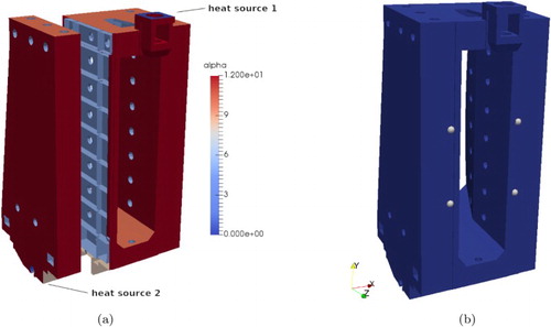
The following numerical experiments are based on the geometry of the prototypical Auerbach ACW 630 machine column shown in Figure 1(b). The material constants are given in Table 1. Notice that the heat transfer coefficient varies over different parts of the boundary, classified according to the orientation of the outer surface normal; see Figure 2(a). The machine column experiences the influence of two heat sources, see again Figure 2(a). One source originates from an electric drive mounted on the top of the machine column (surface part ${\mathrm{\Gamma }}_{r1}$), while the other source represents the spindle driving the horizontal movement of the column (${\mathrm{\Gamma }}_{r2}$).

Figure 2. Heat sources, values of heat transfer coefficient and TCP location. (a) Heat sources and heat transfer coefficient. (b) Mounting points determining the TCP location.

The location of the heat sources enters the matrix $B_{\mathrm{th}}$ in (2(2) $\begin{array}{rl}{E}_{\mathrm{th}}\dot{T}& =A_{\mathrm{th}}T+B_{\mathrm{th}}z\\ T(\cdot ,0)& =T_0\end{array}$(2) ) and (6(6) $\left[\begin{array}{cc}{E}_{\mathrm{th}}& 0\\ 0& 0\end{array}\right]\left[\begin{array}{c}\dot{T}\\ \dot{u}\end{array}\right]=\left[\begin{array}{cc}{A}_{\mathrm{th}}& 0\\ A_{\mathrm{thel}}& -A_{\mathrm{el}}\end{array}\right]\left[\begin{array}{c}T\\ u\end{array}\right]+\left[\begin{array}{c}{B}_{\mathrm{th}}\\ 0\end{array}\right]z\iff E\dot{x}=Ax+Bz$(6) ) and thus it has an impact on all reduced-order models. Note that the number of inputs is m=3, because the ambient temperature $T_{\mathrm{ref}}$ is considered as an input in order to achieve a linear (as opposed to affine) control system (2(2) $\begin{array}{rl}{E}_{\mathrm{th}}\dot{T}& =A_{\mathrm{th}}T+B_{\mathrm{th}}z\\ T(\cdot ,0)& =T_0\end{array}$(2) ). For the generation of the snapshots needed for the simulation based POD MOR technique, a typical thermal load cycle has to be specified in addition to the initial temperature. In (1(1) $\begin{array}{rl}\rho c_p\dot{T}-\mathrm{div}\left(\lambda \mathrm{\nabla }T\right)& =0\text{in }\mathrm{\Omega }\times (0,t_{\mathrm{end}})\\ \lambda \frac{\mathrm{\partial }}{\mathrm{\partial }n}T+\alpha \left(x\right)(T-T_{\mathrm{ref}})& =r(x,t)\text{on }\mathrm{\Gamma }\times (0,t_{\mathrm{end}})\\ T(\cdot ,0)& =T_0\text{in }\mathrm{\Omega }\end{array}\}$(1) ) the load profile (25) $r(x,t)=\{\begin{array}{ll}6700{\mathrm{W}\mathrm{m}}^{-2}& \text{if }x\in {\mathrm{\Gamma }}_{r1}\text{ and }0\mathrm{s}\le t\le 1800\mathrm{s},\\ 2700{\mathrm{W}\mathrm{m}}^{-2}& \text{if }x\in {\mathrm{\Gamma }}_{r2}\text{ and }0\mathrm{s}\le t\le 1800\mathrm{s},\\ 2700{\mathrm{W}\mathrm{m}}^{-2}& \text{if }x\in {\mathrm{\Gamma }}_{r2}\text{ and }3600\mathrm{s}\le t\le 5400\mathrm{s},\\ 6700{\mathrm{W}\mathrm{m}}^{-2}& \text{if }x\in {\mathrm{\Gamma }}_{r1}\text{ and }5400\mathrm{s}<t\le 7200\mathrm{s},\\ 0& \mathrm{else}\end{array}$(25) is used, which represents a realistic machining scenario. This heat source gives rise to a time-dependent control input $z\left(t\right)$ in the semi-discretized models (2(2) $\begin{array}{rl}{E}_{\mathrm{th}}\dot{T}& =A_{\mathrm{th}}T+B_{\mathrm{th}}z\\ T(\cdot ,0)& =T_0\end{array}$(2) ) and (6(6) $\left[\begin{array}{cc}{E}_{\mathrm{th}}& 0\\ 0& 0\end{array}\right]\left[\begin{array}{c}\dot{T}\\ \dot{u}\end{array}\right]=\left[\begin{array}{cc}{A}_{\mathrm{th}}& 0\\ A_{\mathrm{thel}}& -A_{\mathrm{el}}\end{array}\right]\left[\begin{array}{c}T\\ u\end{array}\right]+\left[\begin{array}{c}{B}_{\mathrm{th}}\\ 0\end{array}\right]z\iff E\dot{x}=Ax+Bz$(6) ). The simulation of the temperature equation (2(2) $\begin{array}{rl}{E}_{\mathrm{th}}\dot{T}& =A_{\mathrm{th}}T+B_{\mathrm{th}}z\\ T(\cdot ,0)& =T_0\end{array}$(2) ) was carried out in a time interval $t\in [0\mathrm{s},9000\mathrm{s}]$ with uniform step length $\delta t=60\mathrm{s}$ using the implicit Euler scheme. The initial temperature for these simulations was choosen as $T_0\equiv T_{\mathrm{ref}}$.

The quantity of interest $\mathit{u}\left(x_{\mathrm{TCP}}\right)$ in the estimation problem on which the sensor placement problem is based is the displacement at the so-called TCP. The tip of the main spindle (holding the tool) seen in the left of Figure 1(a) is defined as the TCP. The main spindle assembly is considered as a rigid body which is thermally insulated from the machine column. Consequently, the TCP displacement is determined by the four mounting points of the sledge holding the main spindle, see Figure 2(b). The dependence of $\mathit{u}\left(x_{\mathrm{TCP}}\right)$ on the deflection in the four mounting points is actually nonlinear, but it is replaced by its linearization; see Herzog and Riedel (2015) for details.

5.2. Comparison of MOR techniques for sensor placement

In this section the results of the sensor placement procedure described in Section 3 are presented and compared, using the MOR techniques under consideration. Recall that POD, BT as well as two variants of MM (Padé and IRKA) are considered, as described in Section 4. In each case, the respective reduced basis V was obtained, following which the sequential sensor placement procedure as described in Section 3.3 was carried out, which amounts to solving a sequence of problems (15(:sequential_sensor_placement) $\begin{array}{rl}\underset{x_i\in {\mathrm{\Gamma }}_{\mathrm{finite}}}{\mathrm{Minimize}}& \mathrm{\Psi }\left({\mathrm{Cov}}_{\mathit{u}\left(x_{\mathrm{TCP}}\right)}\right(x_1,\dots ,x_{i-1};x_i\left)\right)\end{array}$(:sequential_sensor_placement) ). The size of the reduced-order model was r=20 and $n_{\mathrm{sensors}}=30$ sensors were placed in each case.

Figure 3 shows the sensor locations obtained. In the case of POD most of the sensors are placed near to the heat sources, see Figure 3(a). The reason for this phenomenon is that the projection subspace associated with the basis matrix V is based solely on simulations of the thermal model (2(2) $\begin{array}{rl}{E}_{\mathrm{th}}\dot{T}& =A_{\mathrm{th}}T+B_{\mathrm{th}}z\\ T(\cdot ,0)& =T_0\end{array}$(2) ). In particular, the relative intensities and locations of the heat sources will strongly influence the computed subspace. Due to the properties of the heat equation and the heat loss through the boundary, the simulation snapshots are almost zero at a certain distance from the heat sources. Therefore the POD basis also shares this property and thus the information gain for temperature measurements far away from the heat sources is negligible.

Figure 3. Optimal sensor locations for the different MOR methods. (a) POD, (b) BT, (c) Padé, (d) IRKA.

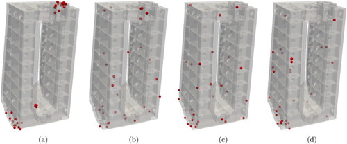
By contrast, the projection matrices V computed from the BT and the two MM procedures are set up independent of the thermal loads and initial condition. Therefore the final sensor locations are spread out more evenly across the machine column's surface, see Figure 3(b–d), to account for all possible heat source trajectories in the image space of $B_{\mathrm{th}}$. Despite its smaller physical extension, it can be observed that the heat source located at the lower part of the machine column attracts a significant amount of sensors. This is quite intuitive since even small deformations at the base of the machine column will naturally be transferred up along the height of the column and thus may have a sizeable influence on the displacement of the TCP.

Recall that BT and IRKA are applied to the reformulation (19(19) $E_{\mathrm{th}}\dot{T}=A_{\mathrm{th}}T+B_{\mathrm{th}}z,y=C_{\mathrm{el}}{A}_{\mathrm{el}}^{-1}{A}_{\mathrm{thel}}T=:\tilde{C}T$(19) ) of the full thermo-elastic model (6(6) $\left[\begin{array}{cc}{E}_{\mathrm{th}}& 0\\ 0& 0\end{array}\right]\left[\begin{array}{c}\dot{T}\\ \dot{u}\end{array}\right]=\left[\begin{array}{cc}{A}_{\mathrm{th}}& 0\\ A_{\mathrm{thel}}& -A_{\mathrm{el}}\end{array}\right]\left[\begin{array}{c}T\\ u\end{array}\right]+\left[\begin{array}{c}{B}_{\mathrm{th}}\\ 0\end{array}\right]z\iff E\dot{x}=Ax+Bz$(6) )–(7(7) $y=Cx$(7) ) and thus the displacement information about the quantity of interest (QOI) is contained in the ROM. In contrast, the POD and Padé procedures solely consider the thermal model (2(2) $\begin{array}{rl}{E}_{\mathrm{th}}\dot{T}& =A_{\mathrm{th}}T+B_{\mathrm{th}}z\\ T(\cdot ,0)& =T_0\end{array}$(2) ).

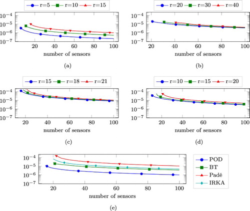
Figure 4 shows the values of the objective function (15(:sequential_sensor_placement) $\begin{array}{rl}\underset{x_i\in {\mathrm{\Gamma }}_{\mathrm{finite}}}{\mathrm{Minimize}}& \mathrm{\Psi }\left({\mathrm{Cov}}_{\mathit{u}\left(x_{\mathrm{TCP}}\right)}\right(x_1,\dots ,x_{i-1};x_i\left)\right)\end{array}$(:sequential_sensor_placement) ) for the different test cases as a function of the number of sensors placed. Smaller values of the objective function indicate less influence of measurement errors on the TCP displacement estimation and thus better estimation precision. Moreover, Figur 4(a–d) shows the influence of the size r of the ROM. For the Padé method, the number p of moments to be matched was chosen as $p\in \{5,6,7\}$. Based on the number of inputs m=3 and the relation r=pm this results in reduced dimensions $r\in \{15,18,21\}$ for the Padé based estimations. Regarding the evolution of the objective function, the qualitative behaviour is very similar for all MOR methods. That is, the best performance in the sense of the experimental design criterion (14(14) ${\mathrm{\Psi }}_A\left(\mathrm{Cov}\right)=\mathrm{trace}\left(\mathrm{Cov}\right){\mathrm{\Psi }}_D\left(\mathrm{Cov}\right)=\ln (det(\mathrm{Cov}\left)\right){\mathrm{\Psi }}_E\left(\mathrm{Cov}\right)={\lambda }_{max}\left(\mathrm{Cov}\right)$(14) ) is achieved for small model sizes. This result was to be expected since smaller models lead to fewer coefficients to be estimated. On the other hand, smaller models lead to larger approximation errors of the ROM compared to the full state model. This is not accounted for in the experimental design criterion. Depending on the needs of the application or the user, a good balance between the two goals has to be found. Figure 4(e) shows a comparison of the different MOR methods for a fixed dimension (r=20) of the reduced systems. Here, the POD based approach shows the best performance with respect to the optimization objective.

Figure 4. Values of the optimal experimental design objective $\mathrm{\Psi }\left(\mathrm{Cov}\right)$ for each MOR technique according to the ROM size r and the number of sensors placed. (a) POD, (b) BT, (c) Padé, (d) IRKA, (e) Comparison for r=20.

Note that the sequence of optimal sensor placement problems (15(:sequential_sensor_placement) $\begin{array}{rl}\underset{x_i\in {\mathrm{\Gamma }}_{\mathrm{finite}}}{\mathrm{Minimize}}& \mathrm{\Psi }\left({\mathrm{Cov}}_{\mathit{u}\left(x_{\mathrm{TCP}}\right)}\right(x_1,\dots ,x_{i-1};x_i\left)\right)\end{array}$(:sequential_sensor_placement) ) operates under the assumption that only temperature states in the range of the respective basis V can occur. To achieve a more meaningful comparison of the four MOR variants, measurements were created from a simulation of the full model. The thermal loads in this simulation differ from those in (25(25) $r(x,t)=\{\begin{array}{ll}6700{\mathrm{W}\mathrm{m}}^{-2}& \text{if }x\in {\mathrm{\Gamma }}_{r1}\text{ and }0\mathrm{s}\le t\le 1800\mathrm{s},\\ 2700{\mathrm{W}\mathrm{m}}^{-2}& \text{if }x\in {\mathrm{\Gamma }}_{r2}\text{ and }0\mathrm{s}\le t\le 1800\mathrm{s},\\ 2700{\mathrm{W}\mathrm{m}}^{-2}& \text{if }x\in {\mathrm{\Gamma }}_{r2}\text{ and }3600\mathrm{s}\le t\le 5400\mathrm{s},\\ 6700{\mathrm{W}\mathrm{m}}^{-2}& \text{if }x\in {\mathrm{\Gamma }}_{r1}\text{ and }5400\mathrm{s}<t\le 7200\mathrm{s},\\ 0& \mathrm{else}\end{array}$(25) ), which were used to create the POD snapshots. The simulation spans the time interval $t\in [0\mathrm{s},7200\mathrm{s}]$ and the thermal loads (26) $r(x,t)=\{\begin{array}{ll}6700{\mathrm{W}\mathrm{m}}^{-2}& \text{if }x\in {\mathrm{\Gamma }}_{r1}\text{ and }0\mathrm{s}\le t\le 2400\mathrm{s},\\ 2700{\mathrm{W}\mathrm{m}}^{-2}& \text{if }x\in {\mathrm{\Gamma }}_{r2}\text{ and }0\mathrm{s}\le t\le 4800\mathrm{s},\\ 6700{\mathrm{W}\mathrm{m}}^{-2}& \text{if }x\in {\mathrm{\Gamma }}_{r1}\text{ and }4800\mathrm{s}<t\le 7200\mathrm{s},\\ 0& \text{else}\end{array}$(26) and an initial temperature of $T_0\equiv T_{\mathrm{ref}}$ were applied. Figure 5(a,b) show the evolution of the simulated TCP deflection compared to its estimated position based on the $n_{\mathrm{sensors}}=30$ optimally placed sensors (in the sense of the approach in Section 3.3) with reduced bases of dimension r=20. The simulated temperature values were evaluated for each ROM at the relevant sensor locations. The TCP displacement estimate was then obtained from solving the least-squares problem (11(11) ${\theta }_{\mathit{u}\left(x_{\mathrm{TCP}}\right)}\left(X\right)=C_{\mathrm{el}}SV{\theta }_{\hat{T}}\left(X\right)=C_{\mathrm{el}}SV(J\left(X{)}^{\mathrm{\top }}J\right(X\left){)}^{-1}J\right(X{)}^{\mathrm{\top }}\tilde{T}$(11) ).

Again, according to the relative errors between simulated and estimated TCP displacements, the POD approach yields the best results in this exercise. The estimation of the TCP displacement associated to the subspace spanned by the Padé procedure shows significant inaccuracies at times $t=120\mathrm{s}$ and $t=4800\mathrm{s}$. 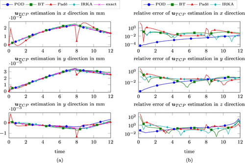This may be due to the fact that the matching of p=7 moments of the transfer function at a single expansion point $s_0=0$ and a resulting reduced dimension r=21, restricted to r=20, cannot sufficiently approximate the actual model behaviour of the original full-order model at those points. Apart from these peaks, the BT, Padé and IRKA based estimates are roughly of the same order of accuracy. Note that the large relative errors at the beginning of the time interval are mainly caused by the fact that the trajectories evolve closely around zero and therefore the relative error is violated by divisions of values that are close to zero. However, it is a well known fact that the ROMs based on POD are, in general, only reliable for operating conditions near those used to generate the POD snapshots. Therefore the experiment was repeated with thermal loads (27) $r_{\mathrm{mod}}(x,t)=\{\begin{array}{ll}3000{\mathrm{W}\mathrm{m}}^{-2}& \text{if }x\in {\mathrm{\Gamma }}_{r1}\text{ and }0\mathrm{s}\le t\le 2400\mathrm{s},\\ 5000{\mathrm{W}\mathrm{m}}^{-2}& \text{if }x\in {\mathrm{\Gamma }}_{r2}\text{ and }0\mathrm{s}\le t\le 4800\mathrm{s},\\ 3000{\mathrm{W}\mathrm{m}}^{-2}& \text{if }x\in {\mathrm{\Gamma }}_{r1}\text{ and }4800\mathrm{s}<t\le 7200\mathrm{s},\\ 0& \text{else}\end{array}$(27) which differ more significantly from the nominal loads (25(25) $r(x,t)=\{\begin{array}{ll}6700{\mathrm{W}\mathrm{m}}^{-2}& \text{if }x\in {\mathrm{\Gamma }}_{r1}\text{ and }0\mathrm{s}\le t\le 1800\mathrm{s},\\ 2700{\mathrm{W}\mathrm{m}}^{-2}& \text{if }x\in {\mathrm{\Gamma }}_{r2}\text{ and }0\mathrm{s}\le t\le 1800\mathrm{s},\\ 2700{\mathrm{W}\mathrm{m}}^{-2}& \text{if }x\in {\mathrm{\Gamma }}_{r2}\text{ and }3600\mathrm{s}\le t\le 5400\mathrm{s},\\ 6700{\mathrm{W}\mathrm{m}}^{-2}& \text{if }x\in {\mathrm{\Gamma }}_{r1}\text{ and }5400\mathrm{s}<t\le 7200\mathrm{s},\\ 0& \mathrm{else}\end{array}$(25) ) than (26(26) $r(x,t)=\{\begin{array}{ll}6700{\mathrm{W}\mathrm{m}}^{-2}& \text{if }x\in {\mathrm{\Gamma }}_{r1}\text{ and }0\mathrm{s}\le t\le 2400\mathrm{s},\\ 2700{\mathrm{W}\mathrm{m}}^{-2}& \text{if }x\in {\mathrm{\Gamma }}_{r2}\text{ and }0\mathrm{s}\le t\le 4800\mathrm{s},\\ 6700{\mathrm{W}\mathrm{m}}^{-2}& \text{if }x\in {\mathrm{\Gamma }}_{r1}\text{ and }4800\mathrm{s}<t\le 7200\mathrm{s},\\ 0& \text{else}\end{array}$(26) ). Figure 6(a,b) show the estimation quality in this case. Here, it was observed that the change of the intensity of the heat sources does not considerably influence the estimations compared to the previous scenario. Only the POD approach performs slightly worse, producing similar error levels to the other MOR methods in this case.

Figure 5. Comparison of the exact (simulated by the full model) TCP displacement with the estimates (11(11) ${\theta }_{\mathit{u}\left(x_{\mathrm{TCP}}\right)}\left(X\right)=C_{\mathrm{el}}SV{\theta }_{\hat{T}}\left(X\right)=C_{\mathrm{el}}SV(J\left(X{)}^{\mathrm{\top }}J\right(X\left){)}^{-1}J\right(X{)}^{\mathrm{\top }}\tilde{T}$(11) ) with simulated measurements at the respective measurement locations (left) with heat sources (26(26) $r(x,t)=\{\begin{array}{ll}6700{\mathrm{W}\mathrm{m}}^{-2}& \text{if }x\in {\mathrm{\Gamma }}_{r1}\text{ and }0\mathrm{s}\le t\le 2400\mathrm{s},\\ 2700{\mathrm{W}\mathrm{m}}^{-2}& \text{if }x\in {\mathrm{\Gamma }}_{r2}\text{ and }0\mathrm{s}\le t\le 4800\mathrm{s},\\ 6700{\mathrm{W}\mathrm{m}}^{-2}& \text{if }x\in {\mathrm{\Gamma }}_{r1}\text{ and }4800\mathrm{s}<t\le 7200\mathrm{s},\\ 0& \text{else}\end{array}$(26) ). Relative errors are shown in the right plot. (a) Estimated and simulated displacements at the TCP. (b) Relative errors.

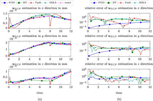
Figure 6. As for Figure 5 using alternative heat sources (27(27) $r_{\mathrm{mod}}(x,t)=\{\begin{array}{ll}3000{\mathrm{W}\mathrm{m}}^{-2}& \text{if }x\in {\mathrm{\Gamma }}_{r1}\text{ and }0\mathrm{s}\le t\le 2400\mathrm{s},\\ 5000{\mathrm{W}\mathrm{m}}^{-2}& \text{if }x\in {\mathrm{\Gamma }}_{r2}\text{ and }0\mathrm{s}\le t\le 4800\mathrm{s},\\ 3000{\mathrm{W}\mathrm{m}}^{-2}& \text{if }x\in {\mathrm{\Gamma }}_{r1}\text{ and }4800\mathrm{s}<t\le 7200\mathrm{s},\\ 0& \text{else}\end{array}$(27) ). (a) Estimated and simulated displacements at the TCP. (b) Relative errors.

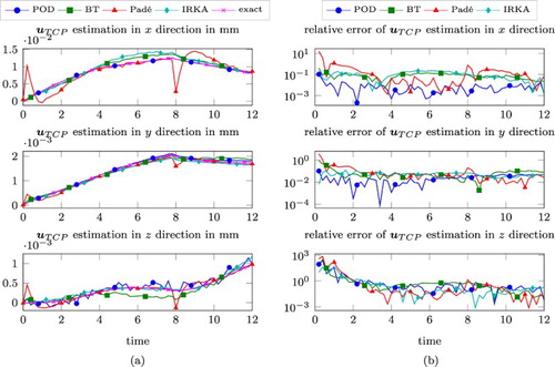
In a final experiment the robustness of the TCP displacement estimation with respect to noisy measurements using a standard deviation of $\sigma =0.1$ is analysed in Figure 7(a,b). The heat sources were chosen as in (26(26) $r(x,t)=\{\begin{array}{ll}6700{\mathrm{W}\mathrm{m}}^{-2}& \text{if }x\in {\mathrm{\Gamma }}_{r1}\text{ and }0\mathrm{s}\le t\le 2400\mathrm{s},\\ 2700{\mathrm{W}\mathrm{m}}^{-2}& \text{if }x\in {\mathrm{\Gamma }}_{r2}\text{ and }0\mathrm{s}\le t\le 4800\mathrm{s},\\ 6700{\mathrm{W}\mathrm{m}}^{-2}& \text{if }x\in {\mathrm{\Gamma }}_{r1}\text{ and }4800\mathrm{s}<t\le 7200\mathrm{s},\\ 0& \text{else}\end{array}$(26) ). The TCP evolution trajectories and the corresponding relative errors again reveal the superiority of the POD approach applied to the optimal experimental design framework, while the other strategies are of the same order of accuracy as before.

Figure 7. As for Figure 5 with heat sources (26(26) $r(x,t)=\{\begin{array}{ll}6700{\mathrm{W}\mathrm{m}}^{-2}& \text{if }x\in {\mathrm{\Gamma }}_{r1}\text{ and }0\mathrm{s}\le t\le 2400\mathrm{s},\\ 2700{\mathrm{W}\mathrm{m}}^{-2}& \text{if }x\in {\mathrm{\Gamma }}_{r2}\text{ and }0\mathrm{s}\le t\le 4800\mathrm{s},\\ 6700{\mathrm{W}\mathrm{m}}^{-2}& \text{if }x\in {\mathrm{\Gamma }}_{r1}\text{ and }4800\mathrm{s}<t\le 7200\mathrm{s},\\ 0& \text{else}\end{array}$(26) ) using noisy measurements. (a) Estimated and simulated displacements at the TCP. (b) Relative errors.

6. Discussion

In this article, an optimal sequential placement strategy for temperature sensors in order to predict thermally induced mechanical deformations from temperature measurements was revisited. To make the sensor placement procedure tractable, MOR was applied either to the temperature equation alone, or to the full thermo-mechanical model. The main focus of this article was to compare the performance of different MOR methods with respect to the sensor placement objective and the prediction quality of the induced displacement estimation using simulated measurements at the optimized sensor positions.

Comparing the simulation results based on the data used as the POD training scenario and a fixed model size of r=20, the POD approach showed the best performance with respect to the experimental design objective as well as the estimation accuracy of the TCP displacement. Considering thermal loads outside the POD training set, as well as for noisy measurement data, the POD, BT, and IRKA based MOR approaches basically show the same behaviour with respect to the estimation accuracy. POD, as a simulation based MOR approach, depends on the snapshot ensemble being sufficiently rich to yield a reliable ROM. Nevertheless, POD was found to work well compared to the other MOR schemes, even under significant perturbations of the heating profile used during the training phase. Interestingly, POD shows best performance with respect to to the prescribed reduced order/number of sensors and the comparison criteria even though it targets only the temperature field and no information about the true QOI (the TCP displacement) is included. POD especially takes into account the explicit influence of the actual acting loads and, according to that, clusters the sensors corresponding to the regions of dominant thermal interest.

The three other MOR methods which were considered do not depend on simulations. Moreover, the BT and IRKA approaches operate on an equivalent reformulation of the full thermo-mechanical model and thus include QOI information. On the other hand, these methods do not consider the actual machining process. Therefore, they are less specialized such that the corresponding ROMs need to be significantly larger in order to achieve comparable performance. Still, for drastically changed machining processes, e.g.  with no action on the lower heat source, they are expected to give much better results than the POD prior to modification, i.e.  regeneration of the POD basis by new training with the changed input situation. However, quantification of the degeneration of the POD model requires further investigation. Out of these methods, the BT and the IRKA MM approaches performed best, and very similarly.

Disclosure statement

No potential conflict of interest was reported by the authors.

ORCID

Peter Benner http://orcid.org/0000-0003-3362-4103

Roland Herzog http://orcid.org/0000-0003-2164-6575

Norman Lang http://orcid.org/0000-0002-9074-0103

Ilka Riedel http://orcid.org/0000-0002-7705-6550

Jens Saak http://orcid.org/0000-0001-5567-9637

Additional information

Funding

This work was supported by two Deutsche Forschungsgemeinschaft (DFG) grants within the Special Research Program SFB/Transregio 96 (Thermo-energetische Gestaltung von Werkzeugmaschinen), which is gratefully acknowledged.

Notes

* An abridged version of the manuscript was submitted to the CIRP sponsored conference on Conference on Thermal Issues in Machine Tools, 2018.

References

- Alonso, A. A., C. E. Frouzakis, and I. G. Kevrikidis. 2004. “Optimal Sensor Placement for State Reconstruction of Distributed Process Systems.” AIChE Journal 50 (7): 1438–1452. doi: 10.1002/aic.10121
- Alonso, A. A., I. G. Kevrekidis, J. R. Banga, and C. E. Frouzakis. 2004. “Optimal Sensor Location and Reduced Order Observer Design for Distributed Process Systems.” Computers & Chemical Engineering 28 (1-2): 27–35. doi: 10.1016/S0098-1354(03)00175-3
- Antoulas, A. C. 2005. Approximation of Large-scale Dynamical Systems. Vol. 6 of Advances in Design and Control. Philadelphia, PA: Society for Industrial and Applied Mathematics (SIAM).
- Armaou, A., and M. A. Demetriou. 2006. “Optimal Actuator/Sensor Placement for Linear Parabolic PDEs Using Spatial Norm.” Chemical Engineering Science 61 (22): 7351–7367. doi: 10.1016/j.ces.2006.07.027
- Benner, P., P. Kürschner, and J. Saak. 2013a. “An Improved Numerical Method for Balanced Truncation for Symmetric Second-order Systems.” Mathematical and Computer Modelling of Dynamical Systems 19 (6): 593–615. doi: 10.1080/13873954.2013.794363
- Benner, P., P. Kürschner, and J. Saak. 2013b. “A Reformulated Low-Rank ADI Iteration with Explicit Residual Factors.” Proceedings in Applied Mathematics and Mechanics 13 (1): 585–586. doi: 10.1002/pamm.201310273
- Benner, P., P. Kürschner, and J. Saak. 2014/15. “Self-generating and Efficient Shift Parameters in ADI Methods for Large Lyapunov and Sylvester Equations.” Electronic Transactions on Numerical Analysis 43: 142–162.
- Benner, P., and A. Schneider. 2013. Balanced Truncation for Descriptor Systems with Many Terminals. Preprint MPIMD/13-17. Max Planck Institute Magdeburg.
- Boley, B. A., and J. H. Weiner. 1960. Theory of Thermal Stresses. New York London: John Wiley & Sons Inc.
- Braess, D. 2007. Finite Elements: Theory, Fast Solvers, and Applications in Solid Mechanics. Cambridge: Cambridge University Press.
- Cohen, K., S. Siegel, and T. McLaughlin. 2006. “A Heuristic Approach to Effective Sensor Placement for Modeling of a Cylinder Wake.” Computers & Fluids 35 (1): 103–120. doi: 10.1016/j.compfluid.2004.11.002
- Enns, D. F. 1984. “Model Reduction with Balanced Realizations: An Error Bound and a Frequency Weighted Generalization.” In Proceedings of the 23rd IEEE Conference on Decision and Control, 127–132. New York: IEEE.
- Eslami, M. R., R. B. Hetnarski, J. Ignaczak, N. Noda, N. Sumi, and Y. Tanigawa. 2013. Theory of Elasticity and Thermal Stresses. Vol. 197 of Solid Mechanics and its Applications. Dordrecht: Springer. Explanations, problems and solutions.
- Fedorov, V. V., and P. Hackl. 1997. Model-oriented Design of Experiments. Vol. 125 of Lecture Notes in Statistics. New York: Springer-Verlag.
- García, M. R., C. Vilas, J. R. Banga, and A. A. Alonso. 2007. “Optimal Field Reconstruction of Distributed Process Systems from Partial Measurements.” Industrial & Engineering Chemistry Research 46 (2): 530–539. doi: 10.1021/ie0604167
- Glover, K. 1984. “All Optimal Hankel-norm Approximations of Linear Multivariable Systems and their L∞-error Bounds.” International Journal of Control 39 (6): 1115–1193. doi: 10.1080/00207178408933239
- Green, K. 2006. “Optimal Sensor Placement for Parameter Identification.” Master thesis, Rice University, Houston.
- Grossmann, C., H.-G. Roos, and M. Stynes. 2007. Numerical Treatment of Partial Differential Equations. Berlin: Springer.
- Gugercin, S., A. C. Antoulas, and C. Beattie. 2008. “H2 Model Reduction for Large-scale Linear Dynamical Systems.” SIAM Journal on Matrix Analysis and Applications 30 (2): 609–638. doi: 10.1137/060666123
- Herzog, R., and I. Riedel. 2015. “Sequentially Optimal Sensor Placement in Thermoelastic Models for Real Time Applications.” Optimization and Engineering 16 (4): 737–766. doi: 10.1007/s11081-015-9275-0
- Kammer, D. C. 1991. “Sensor Placement for On-orbit Modal Identification and Correlation of Large Space Structures.” Journal of Guidance, Control, and Dynamics 14 (2): 251–259. doi: 10.2514/3.20635
- Koevoets, A. H., H. J. Eggink, J. Van der Sanden, J. Dekkers, and T. A. M. Ruijl. 2007. “Optimal Sensor Configuring Techniques for the Compensation of Thermo-elastic Deformations in High-precision Systems.” In Proceedings of the 13th International Workshop on Thermal Investigation of ICs and Systems, 208–213. IEEE.
- Körkel, S., H. Arellano-Garcia, J. Schöneberger, and G. Wozny. 2008. “Optimum Experimental Design for Key Performance Indicators.” Computer Aided Chemical Engineering 25: 575–580. doi: 10.1016/S1570-7946(08)80101-0
- Kunisch, K., and S. Volkwein. 2001. “Galerkin Proper Orthogonal Decomposition Methods for Parabolic Problems.” Numerische Mathematik 90 (1): 117–148. doi: 10.1007/s002110100282
- Kürschner, P. 2016. “Efficient Low-Rank Solution of Large-Scale Matrix Equations.” Dissertation, Otto-von-Guericke-Universität Magdeburg.
- Laub, A., M. Heath, C. Paige, and R. Ward. 1987. “Computation of System Balancing Transformations and Other Applications of Simultaneous Diagonalization Algorithms.” IEEE Transactions on Automatic Control 32 (2): 115–122. doi: 10.1109/TAC.1987.1104549
- Meo, M., and G. Zumpano. 2005. “On the Optimal Sensor Placement Techniques for a Bridge Structure.” Engineering Structures 27 (10): 1488–1497. doi: 10.1016/j.engstruct.2005.03.015
- Mokhasi, P., and D. Rempfer. 2004. “Optimized Sensor Placement for Urban Flow Measurement.” Physics of Fluids 16 (5): 1758–1764. doi: 10.1063/1.1689351
- Moore, B. 1981. “Principal Component Analysis in Linear Systems: Controllability, Observability, and Model Reduction.” IEEE Transactions on Automatic Control 26 (1): 17–32. doi: 10.1109/TAC.1981.1102568
- Saad, Y. 2003. Iterative Methods for Sparse Linear Systems. 2nd ed. Philadelphia: Society for Industrial and Applied Mathematics (SIAM).
- Seber, G. A. F., and C. J. Wild. 2005. Nonlinear Regression. Wiley Series in Probability and Statistics. New York: John Wiley & Sons.
- Sun, H., and O. Büyüköztürk. 2015. “Optimal Sensor Placement in Structural Health Monitoring Using Discrete Optimization.” Smart Materials and Structures 24 (12): 125034. doi: 10.1088/0964-1726/24/12/125034
- Uciński, D. 2005. Optimal Measurement Methods for Distributed Parameter System Identification. Systems and Control Series. Boca Raton, FL: CRC Press.
- Uciński, D., and M. Patan. 2007. “D-optimal Design of a Monitoring Network for Parameter Estimation of Distributed Systems.” Journal of Global Optimization 39 (2): 291–322. doi: 10.1007/s10898-007-9139-z
- Willcox, K. 2006. “Unsteady Flow Sensing and Estimation via the Gappy Proper Orthogonal Decomposition.” Computers & Fluids 35 (2): 208–226. doi: 10.1016/j.compfluid.2004.11.006
- Yi, T.-H., H.-N. Li, and M. Gu. 2011. “Optimal Sensor Placement for Structural Health Monitoring Based on Multiple Optimization Strategies.” The Structural Design of Tall and Special Buildings 20 (7): 881–900. doi: 10.1002/tal.712
- Yildirim, B., C. Chryssostomidis, and G. E. Karniadakis. 2009. “Efficient Sensor Placement for Ocean Measurements Using Low-dimensional Concepts.” Ocean Modelling 27 (3-4): 160–173. doi: 10.1016/j.ocemod.2009.01.001