Robust optimization based on analytical evaluation of uncertainty propagation

ABSTRACT

Optimization under uncertainty requires proper handling of those input parameters that contain scatter. Scatter in input parameters propagates through the process and causes scatter in the output. Stochastic methods (e.g. Monte Carlo) are very popular for assessing uncertainty propagation using black-box function metamodels. However, they are expensive. Therefore, in this article a direct method of calculating uncertainty propagation has been employed based on the analytical integration of a metamodel of a process. Analytical handling of noise variables not only improves the accuracy of the results but also provides the gradients of the output with respect to input variables. This is advantageous in the case of gradient-based optimization. Additionally, it is shown that the analytical approach can be applied during sequential improvement of the metamodel to obtain a more accurate representative model of the black-box function and to enhance the search for the robust optimum.

KEYWORDS:

• Robustness and sensitivity analysis
• uncertainty modeling
• sequential optimization
• metamodel-based optimization

1. Introduction

Optimizing a process using computer simulations requires many evaluations of the model. Those models are generally black-box functions that evaluate the output based on the input parameters. For a computationally expensive model, a metamodel can replace the black-box function to enhance the optimization procedure, since function evaluation on a metamodel is much faster than on the model itself (Koziel, Ciaurri, and Leifsson 2011; Dellino, Kleijnen, and Meloni 2015). A metamodel-based approach is used not only in deterministic optimization but also in optimization under uncertain input parameters (Zhuang, Pan, and Du 2015).

Uncontrollable or difficult-to-control input parameters are a challenge in engineering design and manufacturing. The parameters that can be adjusted to get an optimum output are called design variables. The parameters that are mainly out of control or are difficult to control are called noise variables. Noise variables require thoughtful handling. The main concern is how these affect the response of the process. This problem is very common in various fields of study, including—but not limited to—engineering, physics, biology and economics. For instance, uncertainty analysis has been performed in large-scale energy/economic policy models (Kann and Weyant 2000), zero-defect manufacturing (Myklebust 2013), maintenance modelling (Gao and Zhang 2008), the study of groundwater flow (Dettinger and Wilson 1981), engineering design (Kang, Lee, and Lee 2012), weather forecasting (Palmer 2000) and health related issues (Barchiesi, Kessentini, and Grosges 2011). For this purpose, several uncertainty analysis methods have been developed over the past decades. Monte Carlo (MC) and its variations, perturbation methods (Taylor-series expansion), Gaussian Quadrature (GQ), polynomial chaos and stochastic collocation have been widely used (Lee and Chen 2009). The dimensionality of the problem (Fuchs and Neumaier 2008) and the fidelity of the model (Ng and Willcox 2014) determine the efficiency of these methods.

The goal of robust optimization is to find a design point at which the output is least sensitive to the variation of input noise variables. A typical metamodel-based robust optimization approach, shown in Figure 1, consists of several steps. First, a design of experiments (DOE) is generated (step 1) and the responses of the black-box function are evaluated for the discrete DOE points (step 2). Then a metamodel, which is the mathematical fit of the black-box function, is constructed (Step 3). Considering the uncertainty of noise variables, the characteristics of the response uncertainty is then evaluated (step 4). Then, using a given criterion, the objective function value which should be minimized is calculated and a robust optimum is obtained. The objective function is generally selected as $f\left(\mathbf{x}\right)=\tilde{f}\left(\mu \right(\mathbf{x}),\sigma (\mathbf{x}\left)\right)$ in which $\mu \left(\mathbf{x}\right)$ is the mean of the response and $\sigma \left(\mathbf{x}\right)$ is the standard deviation of the response (step 5). The robust optimum is evaluated on a metamodel of the process. As the metamodel is an approximate representation of the process, reliance on a metamodel might lead to loss of accuracy in the evaluation of the robust optimum. To reduce the prediction error, sequential improvement of the metamodel can be applied (Wiebenga, van den Boogaard, and Klaseboer 2012). For this purpose new points are added to the initial DOE to get an improved metamodel of the process. Improving the metamodel helps to get a more accurate robust optimum of the underlying process. A new infill point is selected in combined design and noise parameter space (step 6) and the black-box output is evaluated at that point (step 7). Then an updated metamodel is fitted to evaluate the objective function value (step 8). One might continue this improvement until a satisfactory level of accuracy is obtained by sequentially adding more infill points.

Figure 1. Steps of robust optimization with sequential improvement.

In recent years, metamodel-based robust optimization has been implemented in a variety of fields to optimize the processes in the presence of unavoidable noise parameters. Sun et al. (2014) applied it to improve the crashworthiness and robustness of a foam-filled thin-walled structure. In that work, the initial DOE comprised 32 sample points generated using the Latin hyper-cube sampling (LHS) approach and 12 sampling points were added by a sequential sampling strategy in a two-dimensional parameter space. They showed the influence of improvement steps on the accuracy of the metamodel and predicted the robust optimum. Choi et al. (2018) implemented a robust optimization method for designing a tandem grating solar absorber. A Kriging method was used to build a metamodel in a five-dimensional input space and uncertainty propagation was evaluated using a genetic algorithm method. It was shown that at the robust optimum design a solar absorptance of greater than 0.92 was achieved with a probability of $90\mathrm{\%}$. That was a significant improvement compared to the reference design in a previous work in which only $22\mathrm{\%}$ of samples could satisfy the same condition. The capability of metamodel-based robust optimization to solve an industrial V-bending process was investigated by Wiebenga, van den Boogaard, and Klaseboer (2012). Various initial DOEs were generated using LHS on a six-dimensional design-noise variable space. A Kriging metamodel was used and uncertainty propagation was evaluated using an MC method. They validated the obtained robust optimum through a metamodel using a large reference data set, constructed by performing 6000 FE simulations.

For each robust optimization step shown in Figure 1, various methods exist and a variety of choices can be combined during the whole procedure (Huang et al. 2006; Marzat, Walter, and Piet-Lahanier 2013; Kitayama and Yamazaki 2014; ur Rehman, Langelaar, and van Keulen 2014). For instance, several methods exist for making an initial DOE such as factorial design, central composite, space filling, and LHS (Cavazzuti 2013). To evaluate noise propagation through a metamodel, various techniques such as Bayesian statistical modeling, the method of moments, MC, analytical integration, and Taylor series approximation can be used (Heijungs and Lenzen 2014; Leil 2014). The computational effort during metamodel-based robust optimization directly depends on the methods used in each step. There are some steps, e.g. the calculation of uncertainty propagation and objective function uncertainty, that occur more frequently than the other steps. The current methods dealing with those steps are not efficient enough.

In this article, an efficient method for the calculation of uncertainty propagation during the search for a robust optimum is presented. This method assesses uncertainty propagation through the analytical integration of the multiplication of metamodel and input noise probability distribution. Moreover, it can evaluate the uncertainty of the objective function value and the derivatives of output with respect to each input variable. This approach is compared with an MC method in terms of efficiency and accuracy. This article is structured as follows: in Section 2, a general approach is presented for calculating uncertainty propagation analytically. In Section 2.4, the parameters for Kriging and radial basis function (RBF) metamodels are derived. Two examples are addressed in Section 3: a Branin function having one design and one noise parameter, and a basketball free throw in windy weather conditions having three design and two noise variables.

2. Analytical approach for evaluating output uncertainty in robust optimization

2.1. Uncertainty propagation

Assume a process that has M inputs and one output. The vector of input variables is considered as $\mathbf{X}\in {\mathbb{R}}^M$, which includes design parameters, $\mathbf{x}\in {\mathbb{R}}^m$, and noise parameters, $\mathbf{z}\in {\mathbb{R}}^n$. Assume that the response of the process, r, is defined as $r=r\left(\mathbf{X}\right)=r\left(\mathbf{x}\mathbf{,}\mathbf{z}\right)$ using a metamodel. The mean and variance of the response are expressed by (1) ${\mu }_r\left(\mathbf{x}\right)={\int }_{\mathbf{z}}r\left(\mathbf{x}\mathbf{,}\mathbf{z}\right)p\left(\mathbf{z}\right)\mathrm{d}\mathbf{z}$(1) (2) ${\sigma }_r^2\left(\mathbf{x}\right)={\int }_{\mathbf{z}}[r\left(\mathbf{x}\mathbf{,}\mathbf{z}\right)-{\mu }_r\left(\mathbf{x}\right){]}^{2}p\left(\mathbf{z}\right)\mathrm{d}\mathbf{z}.$(2) In this equation, $p\left(\mathbf{z}\right)$ is the probability distribution function of the noise parameters. It is assumed that the noise variables are statistically independent. If the noise variables are not statistically independent, this method is still applicable using principal component analysis (PCA) of the input noise. A PCA step should be performed before robust optimization to transform a set of correlated parameters into a set of linearly uncorrelated parameters. More details about employing PCA in robust optimization to decouple the input noise parameters can be found in Wiebenga et al. (2014).

It has been shown that if $r\left(\mathbf{X}\right)$ can be expressed as a sum of tensor-product basis functions the results of univariate integrals can be combined to evaluate multivariate integrals (Chen, Jin, and Sudjianto 2005). Multivariate tensor-product basis functions, $B_i\left(\mathbf{X}\right)$, can be written as a product of M univariate basis functions, $b_i\left(X\right)$: (3) $B_i\left(\mathbf{X}\right)=\prod _{P=1}^M{b}_{iP}\left(X_P\right),$(3) where $b_{iP}\left(X_P\right)$ is a univariate basis function. If a response function $r\left(\mathbf{X}\right)$ can be defined using linear expansion of these multivariate basis functions, it can also be re-written in terms of univariate basis functions as follows: (4) $r\left(\mathbf{X}\right)=a_0+\sum _{i=1}^N{a}_i{B}_i\left(\mathbf{X}\right)=a_0+\sum _{i=1}^N[a_i\prod _{P=1}^M{b}_{iP}\left(X_P\right)].$(4) In this equation, N is the number of multivariate basis functions that are used to describe $r\left(\mathbf{X}\right)$. Most of the metamodels commonly used, e.g. polynomial regression, Kriging and Gaussian RBFs, can be expressed using tensor-product basis functions.

By substituting Equation (4(4) $r\left(\mathbf{X}\right)=a_0+\sum _{i=1}^N{a}_i{B}_i\left(\mathbf{X}\right)=a_0+\sum _{i=1}^N[a_i\prod _{P=1}^M{b}_{iP}\left(X_P\right)].$(4) ) into (1(1) ${\mu }_r\left(\mathbf{x}\right)={\int }_{\mathbf{z}}r\left(\mathbf{x}\mathbf{,}\mathbf{z}\right)p\left(\mathbf{z}\right)\mathrm{d}\mathbf{z}$(1) ), the mean and standard deviation are obtained through (5) ${\mu }_r\left(\mathbf{x}\right)=a_0+\sum _{i=1}^N\{a_i\prod _{p=1}^m{b}_{ip}\left(x_p\right)\prod _{q=1}^n\mathrm{C}{1}_{iq}\},$(5) where C1 depends on the choice of metamodel and probability distribution: (6) $\mathrm{C}{1}_{iq}={\int }_{z_q}{b}_{iq}\left(z_q\right)p\left(z_q\right)\mathrm{d}{z}_q.$(6) The details of derivations can be found in Appendix 1. Similarly, by inserting Equations (4(4) $r\left(\mathbf{X}\right)=a_0+\sum _{i=1}^N{a}_i{B}_i\left(\mathbf{X}\right)=a_0+\sum _{i=1}^N[a_i\prod _{P=1}^M{b}_{iP}\left(X_P\right)].$(4) ) and (5(5) ${\mu }_r\left(\mathbf{x}\right)=a_0+\sum _{i=1}^N\{a_i\prod _{p=1}^m{b}_{ip}\left(x_p\right)\prod _{q=1}^n\mathrm{C}{1}_{iq}\},$(5) ) into Equation (2(2) ${\sigma }_r^2\left(\mathbf{x}\right)={\int }_{\mathbf{z}}[r\left(\mathbf{x}\mathbf{,}\mathbf{z}\right)-{\mu }_r\left(\mathbf{x}\right){]}^{2}p\left(\mathbf{z}\right)\mathrm{d}\mathbf{z}.$(2) ) the standard deviation is calculated using: (7) ${\sigma }_r^2\left(\mathbf{x}\right)=\sum _{i=1}^N\sum _{j=1}^N{a}_i{a}_j\prod _{p=1}^m{b}_{ip}\left(x_p\right)b_{jp}\left(x_p\right)(\prod _{q=1}^n\mathrm{C}{2}_{ijq}-\prod _{q=1}^n\mathrm{C}{1}_{iq}\mathrm{C}{1}_{jq}),$(7) where C2 depends on the choice of metamodel and probability distribution: (8) $\mathrm{C}{2}_{ijq}={\int }_{z_q}{b}_{iq}\left(z_q\right)b_{jq}\left(z_q\right)p\left(z_q\right)\mathrm{d}{z}_q.$(8) Once these coefficients are known for the combination of metamodel and probability distribution, the mean and standard deviation of the output can be evaluated at each design point.

As shown above, C1 and C2 are written in a general form and one needs to choose a metamodel and use proper basis functions, $b_{iP}\left(X_P\right)$, for that metamodel. In addition, the input probability distribution $p\left(\mathbf{z}\right)$ must be specified. C1 and C2 for Kriging metamodels and Gaussian RBFs are evaluated in Section 2.4.

2.2. Analytical gradients

In the case of gradient-based optimization, it is beneficial to provide the gradients analytically. Analytical gradients increase accuracy and computational efficiency, specifically when a large number of input parameters are present. If numerical algorithms are not provided with analytical gradients, finite difference is usually performed to calculate them. When the number of input parameters is large, finite difference is computationally expensive and less accurate than the use of analytical gradients.

Analytical gradients of the mean and standard deviation with respect to each input variable can be calculated by (9) $\frac{\mathrm{d}{\mu }_r\left(\mathbf{x}\right)}{\mathrm{d}{x}_l}=\sum _{i=1}^N\{a_i\prod _{p=1}^m(b_{ip}\left(x_p\right)\frac{\mathrm{d}{b}_{il}\left(x_l\right)/\mathrm{d}{x}_l}{b_{il}\left(x_l\right)})\prod _{q=1}^n\mathrm{C}{1}_{iq}\}$(9) (10) $\begin{array}{rl}\frac{\mathrm{d}{\sigma }_r\left(\mathbf{x}\right)}{\mathrm{d}{x}_l}& =\frac{1}{2{\sigma }_r\left(\mathbf{x}\right)}\sum _{i=1}^N\sum _{j=1}^N{a}_i{a}_j(\prod _{p=1}^m{b}_{ip}\left(x_p\right)b_{jp}\left(x_p\right)\frac{\frac{\mathrm{d}{b}_{il}\left(x_l\right)}{\mathrm{d}{x}_l}{b}_{jl}\left(x_l\right)+b_{il}\left(x_l\right)\frac{\mathrm{d}{b}_{jl}\left(x_l\right)}{\mathrm{d}{x}_l}}{b_{il}\left(x_l\right)b_{jl}\left(x_l\right)})\\ & \times (\prod _{q=1}^n\mathrm{C}{2}_{ijq}-\prod _{q=1}^n\mathrm{C}{1}_{iq}\mathrm{C}{1}_{jq}),\end{array}$(10) where C1 and C2 are as defined in (6(6) $\mathrm{C}{1}_{iq}={\int }_{z_q}{b}_{iq}\left(z_q\right)p\left(z_q\right)\mathrm{d}{z}_q.$(6) ) and (8(8) $\mathrm{C}{2}_{ijq}={\int }_{z_q}{b}_{iq}\left(z_q\right)b_{jq}\left(z_q\right)p\left(z_q\right)\mathrm{d}{z}_q.$(8) ).

2.3. Sequential robust optimization

An optimum design found using the metamodel is not always equal to the optimum of the underlying black-box function. This occurs when the prediction behaviour of the metamodel around the predicted optimum is poor when there are no sampling points around the optimum. Therefore, it is necessary to use an update procedure to improve the metamodel and subsequently obtain an accurate robust optimum. For deterministic optimization, a method has been proposed to take into account both local and global search for new infill points based on expected improvement (Jones, Schonlau, and Welch 1998). The expected improvement is then defined by (11) $\mathrm{EI}\left(\mathbf{x}\right)=(r_{min}^{\ast }-\hat{r})\mathrm{\Phi }\left(\frac{r_{min}^{\ast }-\hat{r}}{\hat{s}}\right)+\hat{s}\phi \left(\frac{r_{min}^{\ast }-\hat{r}}{\hat{s}}\right).$(11) In this equation, φ is the probability distribution of a standardized normal distribution, Φ is the cumulative probability distribution of a standardized normal distribution and $r_{min}^{\ast }$ is the minimum value of the response at the DOE points examined so far. $\hat{r}$ and $\hat{s}$ are the predicted value and uncertainty of the predicted response. A DOE of untried points is formed and the EI is evaluated at those points. The point that has the highest EI value is chosen to be added to the initial DOE and the black-box function is evaluated at that point. Then a new metamodel is fitted based on the updated DOE and responses.

Equation (11(11) $\mathrm{EI}\left(\mathbf{x}\right)=(r_{min}^{\ast }-\hat{r})\mathrm{\Phi }\left(\frac{r_{min}^{\ast }-\hat{r}}{\hat{s}}\right)+\hat{s}\phi \left(\frac{r_{min}^{\ast }-\hat{r}}{\hat{s}}\right).$(11) ) is only useful for deterministic optimization. However, it can be altered to use in a robust optimization procedure (ur Rehman and Langelaar 2016). A new infill point $\mathbf{(}{\mathbf{x}}^{\prime }\mathbf{,}{\mathbf{z}}^{\prime }\mathbf{)}$ must be selected in the combined design and noise space. The robustness measure or objective function value, $f\mathbf{\left(}\mathbf{x}\mathbf{\right)}$, replaces the function value, $r\left(\mathbf{x}\right)$. Moreover, to evaluate $f\mathbf{\left(}\mathbf{x}\mathbf{\right)}$ and get $f_{min}^{\ast }$ one needs to calculate ${\mu }_r\mathbf{\left(}\mathbf{x}\mathbf{\right)}$ and ${\sigma }_r\mathbf{\left(}\mathbf{x}\mathbf{\right)}$ using Equations (1(1) ${\mu }_r\left(\mathbf{x}\right)={\int }_{\mathbf{z}}r\left(\mathbf{x}\mathbf{,}\mathbf{z}\right)p\left(\mathbf{z}\right)\mathrm{d}\mathbf{z}$(1) ) and (2(2) ${\sigma }_r^2\left(\mathbf{x}\right)={\int }_{\mathbf{z}}[r\left(\mathbf{x}\mathbf{,}\mathbf{z}\right)-{\mu }_r\left(\mathbf{x}\right){]}^{2}p\left(\mathbf{z}\right)\mathrm{d}\mathbf{z}.$(2) ). Therefore, the objective function values are not a result of evaluations of the black-box function, but a prediction using a metamodel. Thus, there is a prediction uncertainty at the current best point, which is not the case in the deterministic approach. The minimum of the objective function values obtained from the projection of the DOE points on the design variable domain is then selected as $f_{min}^{\ast }$ that has an uncertainty of ${\hat{s}}^{\ast }$. Suitable estimation for prediction error at any design, $\hat{s}\mathbf{\left(}\mathbf{x}\mathbf{\right)}$, is also required. As the uncertainty measure on the metamodel is dependent on both the design variables and noise variables, there are two main approaches to obtain the uncertainty of the objective function value, ${\hat{s}}_f$. One method is to evaluate an integral over the noise space—evaluating the mean value of the mean square error (MSE) (Wiebenga, van den Boogaard, and Klaseboer 2012; Havinga, van den Boogaard, and Klaseboer 2017)—and the other approach is the minimax robustness criterion (Jurecka 2007; Jurecka, Ganser, and Bletzinger 2007). In this article the first approach is used: (12) ${\hat{s}}_f^2\left(\mathbf{x}\right)={\int }_{\mathbf{z}}{\hat{s}}_f^2(\mathbf{x},\mathbf{z})p\left(\mathbf{z}\right)\mathrm{d}\mathbf{z}.$(12) The influence of the uncertainty of the best point, ${\hat{s}}^{\ast }$, is neglected and the expected improvement is evaluated using Sóbester, Leary, and Keane (2004): (13) $\mathrm{EI}\left(\mathbf{x}\right)=\omega (f_{min}^{\ast }-f)\mathrm{\Phi }(\frac{f_{min}^{\ast }-f}{{\hat{s}}_f})+(1-\omega ){\hat{s}}_f\phi (\frac{f_{min}^{\ast }-f}{{\hat{s}}_f}).$(13) More details about including the influence of ${\hat{s}}^{\ast }$ can be found elsewhere (Jurecka 2007; Jurecka, Ganser, and Bletzinger 2007). The first term in Equation (13(13) $\mathrm{EI}\left(\mathbf{x}\right)=\omega (f_{min}^{\ast }-f)\mathrm{\Phi }(\frac{f_{min}^{\ast }-f}{{\hat{s}}_f})+(1-\omega ){\hat{s}}_f\phi (\frac{f_{min}^{\ast }-f}{{\hat{s}}_f}).$(13) ) is related to local search and the second term is related to global search. One can adjust the search in global and local domains by choosing a proper weight factor such that $0<\omega <1$. In this work $\omega =0.5$ is selected to balance between local and global search. Maximizing the expected improvement using (13(13) $\mathrm{EI}\left(\mathbf{x}\right)=\omega (f_{min}^{\ast }-f)\mathrm{\Phi }(\frac{f_{min}^{\ast }-f}{{\hat{s}}_f})+(1-\omega ){\hat{s}}_f\phi (\frac{f_{min}^{\ast }-f}{{\hat{s}}_f}).$(13) ) leads to the infill point in the design space, ${\mathbf{x}}^{\prime }$. For that design, a point in noise space must be selected to be able to evaluate the black-box function. For this purpose, ${\mathbf{z}}^{\prime }=\arg \underset{\mathbf{z}}{max}\left({\hat{s}}^2\right({\mathbf{x}}^{\prime },\mathbf{z}\left)p\right(\mathbf{z}\left)\right)$ is employed to choose a point in the noise domain. The point $\mathbf{(}{\mathbf{x}}^{\prime }\mathbf{,}{\mathbf{z}}^{\prime }\mathbf{)}$ is then added to the initial DOE, a new metamodel is fitted and the robust optimum is evaluated using the updated metamodel. The sequential improvement stops when the root-mean-square error (RMSE) at the robust optimum (${\hat{s}}_f\left({\mathbf{x}}_{\mathrm{opt}}\right)$) is below a specific threshold.

2.3.1. Analytical approach in sequential robust optimization

Sequential improvement of the metamodel during robust optimization requires prediction of the MSE estimate ${\hat{s}}^2\left(\mathbf{X}\right)={\hat{s}}^2\left(\mathbf{x}\mathbf{,}\mathbf{z}\right)$. For a robust optimization problem, the uncertainty of the objective function must be provided. If the expression of ${\hat{s}}^2$ can be written as a linear expansion of products of univariate basis functions, the evaluation of this integral is also similar to that of (7(7) ${\sigma }_r^2\left(\mathbf{x}\right)=\sum _{i=1}^N\sum _{j=1}^N{a}_i{a}_j\prod _{p=1}^m{b}_{ip}\left(x_p\right)b_{jp}\left(x_p\right)(\prod _{q=1}^n\mathrm{C}{2}_{ijq}-\prod _{q=1}^n\mathrm{C}{1}_{iq}\mathrm{C}{1}_{jq}),$(7) ). The expression of ${\hat{s}}^2$ depends on the choice of metamodel and therefore it will be discussed in the next section.

Up to this section, there has been no assumption on basis functions (choice of metamodel) or probability distribution. One can employ the analytical approach as long as the initial assumptions hold and the multiplication of basis functions in the probability distribution is integrable. If an integral cannot be calculated analytically, numerical quadrature methods can be employed to evaluate the integral. In the next section, the derivations will be provided for Kriging and Gaussian RBF metamodels, combined with the normal probability distribution.

2.4. Evaluation for Kriging and RBF

Calculation of the mean, standard deviation, derivatives and the uncertainty of the objective function value requires the evaluation of C1 and C2. It should be noted that C1 and C2 are only associated with noise parameters and they depend on the choice of metamodel and input probability distribution. In this section, they are evaluated for commonly-used metamodels combined with the normal probability distribution of noise: (14) $\mathcal{N}\left(z_q\right)=\frac{1}{{\sigma }_q\sqrt{2\pi }}\exp \{-\frac{{(z_q-{\mu }_q)}^2}{2{\sigma }_q^2}\},$(14) where ${\mu }_q$ and ${\sigma }_q$ are the mean and standards deviation of the input noise data.

An ordinary Kriging metamodel is described by (15) $r\left(\mathbf{X}\right)={\alpha }_0+\mathbf{r}\left(\mathbf{X}{)}^{\mathrm{T}}{\mathbf{R}}^{-1}\right({\mathbf{y}}_0-{\alpha }_0\mathbf{1})={\alpha }_0+\mathbf{r}(\mathbf{X}{)}^{\mathrm{T}}\mathit{\kappa }={\alpha }_0+\sum _{i=1}^N{\kappa }_i\prod _{P=1}^M{b}_{iP}\left({\mathrm{X}}_P\right).$(15) In this equation, $\mathbf{R}$ contains the correlations between all DOE points. The basis functions for Kriging are (16) $b_{iP}\left({\mathrm{X}}_P\right)=\exp \{-{\theta }_P^2({\mathrm{X}}_P-{\mathrm{X}}_{iP}{)}^2\},$(16) where the values for ${\theta }_P$ are obtained from fitting the Kriging metamodel.

To find the characteristics of the output probability distribution, a normal probability distribution is assumed as input. Considering these assumptions, $C{1}_{iq}$ and $C{2}_{ijq}$ for the Kriging metamodel are (17) $\mathrm{C}{1}_{iq}=\frac{1}{\sqrt{2{\sigma }_q^2{\theta }_q^2+1}}\exp \{\frac{-{\theta }_q^2}{2{\sigma }_q^2{\theta }_q^2+1}({\mu }_q-z_{iq}{)}^2\}$(17) (18) $\mathrm{C}{2}_{ijq}=\frac{1}{\sqrt{4{\sigma }_q^2{\theta }_q^2+1}}\exp \{\frac{-{\theta }_q^2}{4{\sigma }_q^2{\theta }_q^2+1}[({\mu }_q-z_{iq}{)}^2+({\mu }_q-z_{jq}{)}^2+2{\sigma }_q^2{\theta }_q^2(z_{iq}-z_{jq}{)}^2]\}.$(18) For universal Kriging that has a linear trend, the linear part can be evaluated separately. For more detail, the reader is referred to Appendix 2.

The basis functions for RBF are (19) $b_{iP}\left({\mathrm{X}}_P\right)=\exp \{-\frac{{\theta }_P^2}{2{\tau }_i^2}({\mathrm{X}}_P-{\mathrm{X}}_{iP}{)}^2\}.$(19) In these equations, ${\theta }_P$ and ${\tau }_i$ are the parameters obtained from fitting a Gaussian RBF model. The main difference between RBF and Kriging is that the weights in RBF are assigned for each basis function and variable, whereas those weights in a Kriging model are assigned to each variable. More details about fitting and RBF model can be found elsewhere (Havinga, van den Boogaard, and Klaseboer 2017). $C{1}_{iq}$ and $C{2}_{ijq}$ for RBF are (20) $\mathrm{C}{1}_{iq}=\frac{1}{\sqrt{\frac{{\sigma }_q^2{\theta }_q^2}{{\tau }_i^2}+1}}\exp \{\frac{-{\theta }_q^2}{(2{\sigma }_q^2{\theta }_q^2+2{\tau }_i^2)}({\mu }_q-z_{iq}{)}^2\}$(20) (21) $\begin{array}{rl}\mathrm{C}{2}_{ijq}& =\frac{{\tau }_i{\tau }_j}{\sqrt{{\theta }_q^2{\sigma }_q^2{\tau }_i^2+{\theta }_q^2{\sigma }_q^2{\tau }_j^2+{\tau }_i^2{\tau }_j^2}}\exp \{\frac{-{\theta }_q^2}{2({\theta }_q^2{\sigma }_q^2{\tau }_i^2+{\theta }_q^2{\sigma }_q^2{\tau }_j^2+{\tau }_i^2{\tau }_j^2)}\\ & \times [{\tau }_i^2({\mu }_q-z_{jq}{)}^2{\tau }_j^2({\mu }_q-z_{iq}{)}^2+{\theta }_q^2{\sigma }_q^2(z_{iq}-z_{jq}{)}^2]\}.\end{array}$(21) The details on how to evaluate $C{1}_{iq}$ and $C{2}_{ijq}$ for Kriging and RBF metamodels can be found in Appendix 2.

As mentioned earlier, the uncertainty measure for the objective function is another important parameter to obtain during sequential optimization. It depends on the choice of metamodel, and for the Kriging metamodel, (22) ${\hat{s}}_{\mathrm{obj}}^2={\hat{\sigma }}^2-{\hat{\sigma }}^2\sum _{i=1}^N\sum _{j=1}^N{R}_{ij}^{-1}(\prod _{p=1}^m{b}_{ip}{b}_{jp}\prod _{q=1}^n\mathrm{C}{2}_{ijq}).$(22) More details can be found in Appendix 2. In contrast to the Kriging metamodel, RBF does not provide an explicit uncertainty measure. Nevertheless, there are several methods of estimating ${\hat{s}}^2$ for RBF in the literature (see Sóbester, Leary, and Keane 2004; Li et al. 2010; Havinga, van den Boogaard, and Klaseboer 2017) and one common approach is to use the same form as employed for Kriging (Gibbs 1998).

In the next section, the analytical approach for Kriging and RBF will be implemented and the results and predictions presented. A comparison will be made between the analytical approach and MC analyses in terms of accuracy and efficiency.

3. Results and discussion

3.1. Case 1: The Branin function

In this section, the Branin function is used to show the relevance and advantages of using the analytical approach in metamodel-based robust optimization. The exact robust optimum of the Branin function is evaluated and is used for comparison purposes. Branin function has two variables. It is assumed that one variable is the design parameter and the other is the noise variable: (23) $r(x,z)=(z-\frac{5.1x^2}{4{\pi }^2}+\frac{5x}{\pi }-6{)}^2+10(1-\frac{1}{8\pi })\cos \left(x\right)+10,$(23) where $-5\le x\le 10$ and the noise variable, z, follows a normal distribution described by a given mean and standard deviation, $\mathcal{N}(7.5,2.5)$. The function to be minimized is chosen to be $f\left(x\right)={\mu }_r\left(x\right)+3{\sigma }_r\left(x\right)$. The LHS method combined with full factorial design (FFD) is used to generate 14 DOE points. This is done by generating 10,000 various DOE sets using LHS, merging each one with FFD, and evaluating the minimum distance between all DOE points in each set. Among these 10,000 DOE sets, the one that has the biggest minimum distance is selected as the final DOE. Branin function values are evaluated at those points. Both Kriging and Gaussian RBF are used to fit the metamodel. For uncertainty propagation, both MC and analytical methods are employed. 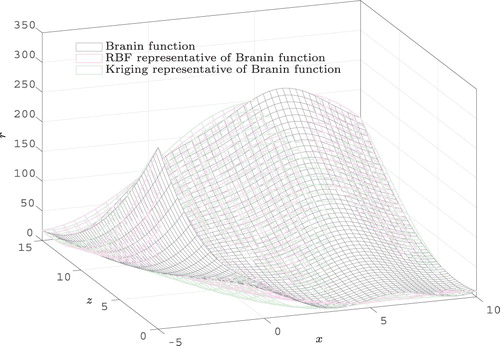It must be noted that Equation (23(23) $r(x,z)=(z-\frac{5.1x^2}{4{\pi }^2}+\frac{5x}{\pi }-6{)}^2+10(1-\frac{1}{8\pi })\cos \left(x\right)+10,$(23) ) is used to find the reference robust optimum. This reference value is used to compare the accuracy of robust optima obtained using MC and the analytical method on metamodels of the Branin function, while in practice the underlying mathematical description of the response might be unknown (Black-box function evaluation). The Branin function and its representative metamodels are illustrated in Figure 2. The sequential quadratic programming (SQP) method is used to find the robust optimum (Cheng and Li 2015).

Figure 2. The Branin function and its representative metamodels.

To minimize the objective function, the algorithm must be supplied with ${\mu }_r\left(x\right)$ and ${\sigma }_r\left(x\right)$. Figure 3 shows the obtained values for ${\mu }_r\left(x\right)$ and ${\sigma }_r\left(x\right)$ using the MC method and the analytical approach. Owing to the randomness of MC sampling, runs using various MC samples using the same metamodel lead to different results. Small MC sampling leads to large deviations in the prediction. It has been suggested that the number of samples for crude MC analysis should be between 100 and 1000 for each dimension (Kleijnen 2007; Bucher 2009). This range balances accuracy versus computational effort. Therefore, in this article these sample sizes are used. Even though increasing the sample size in the noise domain reduces the deviations, they never vanish. In contrast, the consistency of the analytical approach is a big advantage in comparison with stochastic methods such as MC. Additionally, a bigger sample size in the noise domain greatly increases the computational cost. The ratio of calculation time between analytical and MC methods to obtain various output distribution characteristics is shown in Figure 4. Although the computational effort is comparable for small MC samples, increased computational time specifically in high-dimensional problems is inevitable when using a larger MC sample size.

Figure 3. Comparison of mean and standard deviation in the design space obtained using analytical and MC methods for a Kriging metamodel.

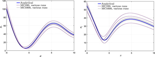
Figure 4. Calculation time ratio for various output distribution characteristics.

Most nonlinear optimization algorithms require derivatives. Providing analytical gradients in the case of gradient-based optimization has significant influence on accuracy and computational efficiency. Approximation methods such as finite difference are widely used to obtain those gradients. However, providing analytical gradients improves the computational efficiency by diminishing unnecessary function evaluations that are required to obtain gradients numerically (Nocedal and Wright 1999). Using the analytical method, second order derivatives (Hessians) of a function can be obtained by using a similar approach if required.

Figure 5 shows a comparison between gradients obtained using finite difference/MC and the analytical approach. As shown here, an accurate and stable gradient is calculated with minimal computational effort.

Figure 5. Comparison of gradients of mean and standard deviation on design space obtained using analytical and MC method for Kriging metamodel.

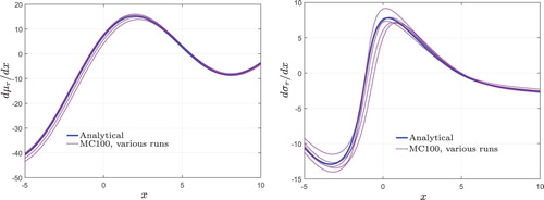
Figure 6 shows the analytical mean, standard deviation, gradient of the mean, and gradient of the standard deviation predicted for RBF. For comparison purposes, MC predictions are also illustrated. It is apparent that the predictions of RBF are different from those of Kriging even though both Kriging and RBF metamodels represent the same function. However, they are essentially different owing to dissimilar parametrizations during the fitting as mentioned in Section 2.4. The predicted trends in the design space for the mean, standard deviation, gradient of the mean and gradient of the standard deviation look similar, but there are basic differences originating from the fitting of the parameters. These differences influence the evaluation of the robust optimum.

Figure 6. Comparison of mean, standard deviation, gradient of mean, and gradient of standard deviation on design space obtained using analytical and MC method for RBF metamodel.

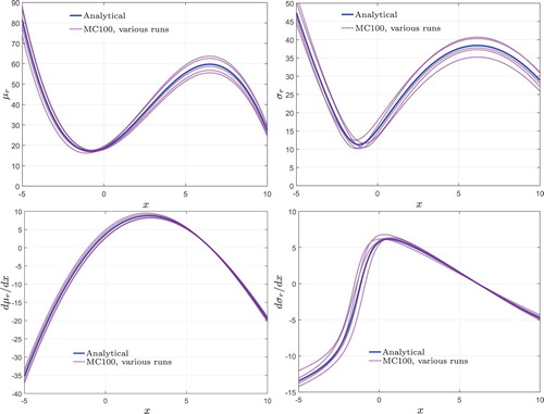
Figure 7 shows the prediction of the uncertainty of the objective function, $\hat{s}\left(x\right)$, using the Kriging model. This figure shows that MC prediction of $\hat{s}\left(x\right)$ mostly underpredicts $\hat{s}\left(x\right)$ values compared to the analytical approach. An improved prediction of $\hat{s}\left(x\right)$ is very important as this value is calculated during each step of the sequential improvement to maximize expected improvement. A better prediction of expected improvement increases the efficiency of the metamodel update by selecting a proper infill point.

Figure 7. Comparison of objective function uncertainty obtained using analytical and MC methods for the Kriging metamodel.

Sequential improvement using the criterion of Equation (13(13) $\mathrm{EI}\left(\mathbf{x}\right)=\omega (f_{min}^{\ast }-f)\mathrm{\Phi }(\frac{f_{min}^{\ast }-f}{{\hat{s}}_f})+(1-\omega ){\hat{s}}_f\phi (\frac{f_{min}^{\ast }-f}{{\hat{s}}_f}).$(13) ) tends to add points that are close to each other. This happens when the sequential improvement is repeated several times and the algorithm finds a candidate optimum. Therefore, besides the initial DOE, there is a cloud of points near to the candidate optimum. In this way, the correlation matrix becomes nearly singular and there are methods to deal with that (Jones, Schonlau, and Welch 1998). A method to avoid sampling nearby points is to use a criterion for global optimization such that it samples on sparsely-sampled regions (Sasena, Papalambros, and Goovaerts 2002). Another approach is to adjust the weight factor in the expected improvement criterion in Equation (13(13) $\mathrm{EI}\left(\mathbf{x}\right)=\omega (f_{min}^{\ast }-f)\mathrm{\Phi }(\frac{f_{min}^{\ast }-f}{{\hat{s}}_f})+(1-\omega ){\hat{s}}_f\phi (\frac{f_{min}^{\ast }-f}{{\hat{s}}_f}).$(13) ) to balance the sampling in a local or global trend (Sóbester, Leary, and Keane 2004).

Using RBF can avoid the above-mentioned problem by assigning each basis function with its own shape parameter, τ, in (19(19) $b_{iP}\left({\mathrm{X}}_P\right)=\exp \{-\frac{{\theta }_P^2}{2{\tau }_i^2}({\mathrm{X}}_P-{\mathrm{X}}_{iP}{)}^2\}.$(19) ). This parameter can be chosen to be correlated with the scaled distance to the nearest neighbour and so avoid a badly-conditioned correlation matrix (Havinga, van den Boogaard, and Klaseboer 2017). Nevertheless, RBF does not include explicit uncertainty measure as Kriging does. Therefore, in this work sequential optimization is only used with the Kriging metamodel.

As the main goal of optimization is to minimize the objective function value, Table 1 shows the objective function values obtained from various approaches. The reference optimum from analytical assessment of the Branin function is at x=−1.12, which has an objective function value of f=47.97. Each MC run using the same metamodel leads to a different robust optimum value and location.

Table 1. Comparison of objective function value and the robust design for various metamodels and approaches without sequential improvement.

	Kriging		RBF
	$x_{\mathrm{optimum}}$	$f_{\mathrm{optimum}}$	$x_{\mathrm{optimum}}$	$f_{\mathrm{optimum}}$
Analytical	−1.02	44.5	−1.10	51.13
MC100 $\mathrm{\#}$1	−1.42	47.10	−1.71	47.45
MC100 $\mathrm{\#}$2	−0.95	44.14	−0.98	45.69
MC100 $\mathrm{\#}$3	−0.67	42.25	−0.66	50.35
MC1000 $\mathrm{\#}$1	−0.94	43.94	−1.06	51.83
MC1000 $\mathrm{\#}$2	−1.06	41.07	−1.02	52.26
MC1000 $\mathrm{\#}$3	−1.09	40.80	−1.19	47.41

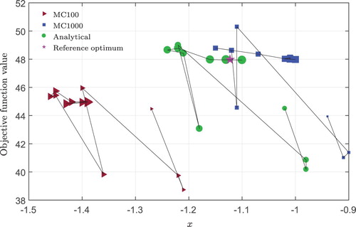
The difference between the reference robust optimum and predicted optimum location and value might decrease if the metamodel is updated properly. Sequential improvement of the metamodel is necessary to obtain a more accurate prediction of the process response specifically around the optimum and consequently to obtain a more accurate robust optimum. Figure 8 shows the improvement of the prediction of the optimum design and objective function values by increasing the number of sequential improvement steps. Each marker shows the optimum design and objective function value after a sequential optimization step. To follow the sequence of improvement, the small markers indicate the beginning of the sequential improvement process, and as the sequential improvement progresses they become larger in size. An improvement in prediction is not always expected, owing to uncertainties (Jurecka 2007). The star mark shown in Figure 8 is the reference optimum. The MC method using 100 samples has quite big deviations in the prediction of both optimum design and objective function values even after sequential improvement. The prediction error decreases by increasing the MC samples to 1000. It is interesting to see that at some point the predicted optimum arrives in the vicinity of the reference optimum. However, by continuing the sequential improvement, the predicted optimum moves away from the reference optimum and converges to a more distant design point. The capability of the analytical approach in predicting the robust optimum is apparent from this figure. Even though the algorithm detects distant designs as candidate optima, e.g. x=−1.24 and x=−1.05, the next try makes sure that those are not the optimum and the algorithm converges towards the reference robust optimum. In addition to that, fewer steps are required to find the robust optimum compared to the MC method. As the predictions of the mean, standard deviation and $\hat{s}$ are more accurate than those found using the MC method, the search for the robust optimum using the analytical method is more efficient.

Figure 8. Improving the prediction of optimum design and objective function values by increasing the number of sequential improvement steps using the Kriging metamodel.

The error in the prediction of the optimum design and objective function values after sequential improvement is shown in Table 2. A bigger MC sample does not always guarantee a better prediction of the optimum design and objective function values. This is due to the fact that the results of MC are sample dependent. Even for the same sample size, there is the possibility of deviations. However, the spread decreases as the MC sample becomes bigger.

Table 2. Comparison of accuracy between the analytical and MC methods for predicting the optimum design and objective function values.

	Reference value	Analytical	MC100	MC1000
x	−1.12	−1.13	−1.39	−1.01
f	47.97	47.96	44.92	48.03
No. of improve-ment steps	–	11	14	15

3.2. Case 2: A basketball free throw in windy weather conditions

In this section, the proposed approach is used to find an optimized setting for a basketball free throw in windy weather conditions. Figure 9 shows the projectile motion of a basketball in the x–z-plane. The design parameters for this problem are initial velocity, $V_0$, throw angle in the x–z-plane, ${\theta }_{xz}$, and throw angle in the x–y-plane, ${\theta }_{xy}$. A side wind is considered as noise during the projectile motion of the basketball. Assuming that the side wind is blowing in the $+y$-direction, a negative throw angle ${\theta }_{xy}$ is required to compensate for the effects of wind. Wind magnitude, $V_w$, and the angle of wind in the x–y-plane, ${\gamma }_w$, are considered as noise variables. The ranges of these parameters are mentioned in Tables 3 and 4.

Figure 9. Projectile motion of a basketball in the x–z-plane.

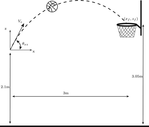
Table 3. Design parameters in basketball free throw.

Design parameter	Lower bound	Upper bound
$V_0$ (m/s)	6.5	7.5
${\theta }_{xz}$ (deg)	55	70
${\theta }_{xy}$ (deg)	−20	−10

Table 4. Noise variables in basketball free throw.

Noise variable	Mean (${\mu }_z$)	St.dev. (${\sigma }_z$)	${\mu }_z-3{\sigma }_z$	${\mu }_z+3{\sigma }_z$
$V_w$ (m/s)	3	1	0	6
${\gamma }_w$ (deg)	−15	5	−30	0

A simulation of this problem gives the final coordinates of the centre of the ball in the x–y-plane at the height of the hoop ($x_f,y_f;z=3.05$) as well as the angle of approach towards the hoop, ${\beta }_{xy}$. As shown in Figure 10, the angle of approach towards the hoop is an important parameter that determines the success of the throw (Brancazio 1981). A higher throw results in a higher angle of approach and therefore a wider range of success. On the other hand, a higher throw increases the effect of the wind and therefore results in more scatter of the final coordinates. It is expected that a strategy can be found that maximizes the number of successful throws.

Figure 10. Side and top view of the hoop and the area of successful approach.

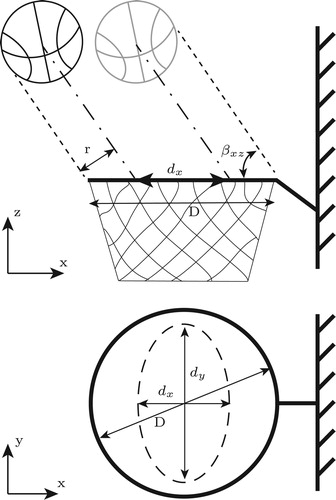
The simulation results are combined in one output parameter, p, that measures the success of the throw: (24) $p=\frac{(x_f-3{)}^2}{d_x^2}+\frac{(y_f{)}^2}{d_y^2},$(24) where (25) $\begin{array}{rl}{d}_x& =D-\frac{2r}{\sin \left({\beta }_{xz}\right)}\\ d_y& =D-\frac{2r}{\sin \left({\beta }_{xy}\right)}.\end{array}$(25) In these equations, $d_x$ and $d_y$ determine the range of successful approaches to the hoop and they depend on the angle of approach towards the hoop as shown in Figure 10 (Brancazio 1981). The lower the value of p, the more successful the throw. The goal is to obtain a setting of design parameters in which p has a minimum value and variation in the windy situation to guarantee the highest rate of success. Therefore, $f\left(\mathbf{x}\right)={\mu }_p\left(\mathbf{x}\right)+3{\sigma }_p\left(\mathbf{x}\right)$ is used as the objective function during robust optimization.

A total of 132 DOE points in the five-dimensional design–noise space is generated based on combined LHS and FFD. The Kriging model is used to build the metamodel and sequential improvement is employed to improve the search for the robust optimum. Table 5 shows the throw setting in windy weather conditions that has the least sensitivity to wind. As discussed in the previous section, MC results fluctuate around the results obtained by the exact analytical method. To investigate the accuracy of the optimum, simulations are done for both MC and the analytical approach in the predicted robust optimum setting. The final coordinates are plotted in Figure 11. 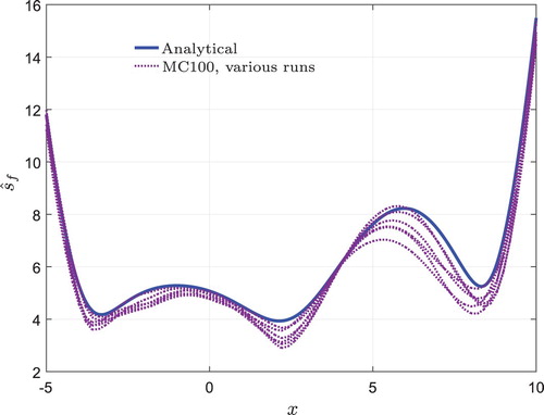This figure shows the top view of the basket and the dotted ellipse represents $d_x$ and $d_y$, which determine the range of successful throws. Inspecting the results obtained by three MC samples of size 100 does not show a reliable prediction in most cases. When the MC sample size increases to 1000, the robust optimum predicted is slightly improved but at the expense of extra computational effort. Simulation of multiple basketball throws in the robust optimum setting found by the analytical approach indicates the consistency and success of this method in high-dimensional problems. Additionally, the computational effort to find the robust optimum is much less compared to MC.

Figure 11. Multiple throws at the robust optimum setting obtained using three different MC100 samples (left), three different MC1000 samples (middle), and the analytical method (right).

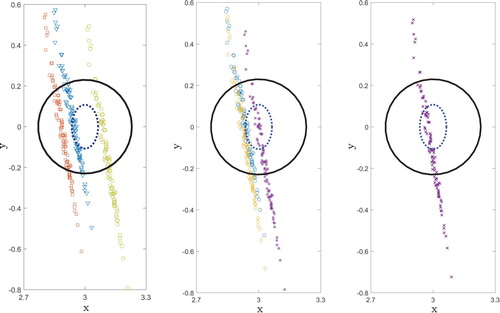
Table 5. Comparison of objective function values and the setting of robust design for various approaches without sequential improvement.

	Optimum throw setting
	$V_0$	${\theta }_{xz}$	${\theta }_{xy}$	$f_{\mathrm{optimum}}$
Analytical	6.92	60.23	−16.25	9.29
MC100 $\mathrm{\#}1$	6.82	60.13	−14.17	6.64
MC100 $\mathrm{\#}2$	7.03	59.74	−17.07	18.47
MC100 $\mathrm{\#}3$	6.74	58.96	−12.67	4.81
MC1000 $\mathrm{\#}1$	6.73	58.67	−11.99	4.54
MC1000 $\mathrm{\#}2$	6.94	59.58	−17.24	12.02
MC1000 $\mathrm{\#}3$	6.88	60.38	−15.47	7.78

Using these examples, it is shown that the analytical approach for uncertainty evaluation can be used during robust optimization of a black-box function. Although some methods have been proposed recently to enhance MC predictability and accuracy (Rajabi, Ataie-Ashtiani, and Janssen 2015), the analytical approach has significant advantages for use in the robust optimization procedure.

4. Conclusions

A sequentially-improved robust optimization technique has been studied using an analytical approach for the evaluation of uncertainty propagation. Robust design in the presence of uncertainties was obtained for Kriging and RBF metamodels, and the results compared with Monte Carlo methods in terms of accuracy and efficiency.

It has been shown that analytical evaluation used in robust optimization is capable of predicting uncertainty propagation more accurately and consistently with minimal computational effort. In addition, analytical evaluation provides the analytical gradients (and analytical Hessians if required), which is a big advantage during gradient-based optimization. Moreover, sequential improvement employing the analytical approach for Kriging metamodels improves prediction of the robust optimum and requires fewer improvement steps.

Disclosure statement

No potential conflict of interest was reported by the authors.

Additional information

Funding

This research was carried out under project number F22.1.13506 in the framework of the Partnership Program of the Materials innovation institute M2i (www.m2i.nl) and the Foundation of Fundamental Research on Matter (FOM) (www.fom.nl), which is part of the Netherlands Organization for Scientific Research (www.nwo.nl).

Appendices

Appendix 1. General approach for propagation of mean and variance

Derivation of mean propagation from (5(5) ${\mu }_r\left(\mathbf{x}\right)=a_0+\sum _{i=1}^N\{a_i\prod _{p=1}^m{b}_{ip}\left(x_p\right)\prod _{q=1}^n\mathrm{C}{1}_{iq}\},$(5) ): (A1) $\begin{array}{rl}{\mu }_r\left(\mathbf{x}\right)& =\int r\left(\mathbf{x}\mathbf{,}\mathbf{z}\right)\mathcal{N}\left(\mathbf{z}\right)\mathrm{d}\mathbf{z}=\int r\left(\mathbf{x}\mathbf{,}\mathbf{z}\right)\prod _{q=1}^n\left[\mathcal{N}\right(z_q\left)\mathrm{d}{z}_q\right]\\ & =\int \{a_0+\sum _{i=1}^N[a_i\prod _{P=1}^M{b}_{iP}\left(X_P\right)]\}\prod _{q=1}^n\left[\mathcal{N}\right(z_q\left)\mathrm{d}{z}_q\right]\\ & =\int \{a_0+\sum _{i=1}^N[a_i\prod _{p=1}^m{b}_{ip}\left(x_p\right)\prod _{q=1}^n{b}_{iq}\left(z_q\right)]\}\prod _{q=1}^n\left[\mathcal{N}\right(z_q\left)\mathrm{d}{z}_q\right]\\ & =a_0+\sum _{i=1}^N\{a_i\prod _{p=1}^m{b}_{ip}\left(x_p\right)\prod _{q=1}^n[\int b_{iq}\left(z_q\right)\mathcal{N}\left(z_q\right)\mathrm{d}{z}_q]\}\\ & =a_0+\sum _{i=1}^N\{a_i\prod _{p=1}^m{b}_{ip}\left(x_p\right)\prod _{q=1}^n\mathrm{C}{1}_{iq}\}.\end{array}$(A1) Derivation of variance propagation from (7(7) ${\sigma }_r^2\left(\mathbf{x}\right)=\sum _{i=1}^N\sum _{j=1}^N{a}_i{a}_j\prod _{p=1}^m{b}_{ip}\left(x_p\right)b_{jp}\left(x_p\right)(\prod _{q=1}^n\mathrm{C}{2}_{ijq}-\prod _{q=1}^n\mathrm{C}{1}_{iq}\mathrm{C}{1}_{jq}),$(7) ): (A2) $\begin{array}{rl}{\sigma }_r^2\left(\mathbf{x}\right)& =\int \left[r\right(\mathbf{x}\mathbf{,}\mathbf{z})-{\mu }_r(\mathbf{x}\left){]}^2\mathcal{N}\right(\mathbf{z})\mathrm{d}\mathbf{z}\\ & =\int r\left(\mathbf{x}\mathbf{,}\mathbf{z}{)}^2\mathcal{N}\right(\mathbf{z})\mathrm{d}\mathbf{z}-2{\mu }_r(\mathbf{x})\int r(\mathbf{x}\mathbf{,}\mathbf{z}\left)\mathcal{N}\right(\mathbf{z})\mathrm{d}\mathbf{z}+{\mu }_r(\mathbf{x}{)}^2\int \mathcal{N}\left(\mathbf{z}\right)\mathrm{d}\mathbf{z}\\ & =\int r\left(\mathbf{x}\mathbf{,}\mathbf{z}{)}^2\mathcal{N}\right(\mathbf{z})\mathrm{d}\mathbf{z}-{\mu }_r(\mathbf{x}{)}^2\\ & =\int [\sum _{i=1}^N{a}_i\prod _{P=1}^{m+n}{b}_{iP}\left(X_P\right){]}^2\prod _{q=1}^n\left[\mathcal{N}\right(z_q\left)\mathrm{d}{z}_q\right]-[\sum _{i=1}^N{a}_i\prod _{p=1}^m{b}_{ip}\left(x_p\right)\prod _{q=1}^n\mathrm{C}{1}_{iq}{]}^2\\ & =\int [\sum _{i=1}^N\sum _{j=1}^N{a}_i{a}_j\prod _{P=1}^{m+n}{b}_{iP}\left(X_P\right)b_{jP}\left(X_P\right)]\prod _{q=1}^n\left[\mathcal{N}\right(z_q\left)\mathrm{d}{z}_q\right]\\ & -\sum _{i=1}^N\sum _{j=1}^N[a_i{a}_j\prod _{p=1}^m{b}_{ip}\left(x_p\right)b_{jp}\left(x_p\right)\prod _{q=1}^n\mathrm{C}{1}_{iq}\mathrm{C}{1}_{jq}]\\ & =\sum _{i=1}^N\sum _{j=1}^N{a}_i{a}_j\prod _{p=1}^m{b}_{ip}\left(x_p\right)b_{jp}\left(x_p\right)[\prod _{q=1}^n\int b_{iq}\left(z_q\right)b_{jq}\left(z_q\right)\mathcal{N}\left(z_q\right)\mathrm{d}{z}_q-\prod _{q=1}^n\mathrm{C}{1}_{iq}\mathrm{C}{1}_{jq}]\\ & =\sum _{i=1}^N\sum _{j=1}^N{a}_i{a}_j\prod _{p=1}^m{b}_{ip}\left(x_p\right)b_{jp}\left(x_p\right)[\prod _{q=1}^n\mathrm{C}{2}_{ijq}-\prod _{q=1}^n\mathrm{C}{1}_{iq}\mathrm{C}{1}_{jq}].\end{array}$(A2) Note that (A3) $(\sum _{i=1}^N{a}_i)(\sum _{j=1}^N{a}_j)=(\sum _{i=1}^N\sum _{j=1}^N{a}_i{a}_j)=(\sum _{k=1}^N{a}_k{)}^2.$(A3)

Appendix 2. Derivations of C1 and C2 for Kriging and RBF

For an ordinary Kriging metamodel, (A4) $r\left(\mathbf{X}\right)={\alpha }_0+\mathbf{r}\left(\mathbf{X}{)}^{\mathrm{T}}{\mathbf{R}}^{-1}\right({\mathbf{y}}_0-{\alpha }_0\mathbf{1})=\hat{\beta }+\mathbf{r}(\mathbf{X}{)}^{\mathrm{T}}\mathit{\kappa }={\alpha }_0+\sum _{i=1}^N{\kappa }_i\prod _{P=1}^M{b}_{iP}\left({\mathrm{X}}_P\right),$(A4) which is in the form of Equation (4(4) $r\left(\mathbf{X}\right)=a_0+\sum _{i=1}^N{a}_i{B}_i\left(\mathbf{X}\right)=a_0+\sum _{i=1}^N[a_i\prod _{P=1}^M{b}_{iP}\left(X_P\right)].$(4) ), considering univariate basis functions as (A5) $b_{iP}\left({\mathrm{X}}_P\right)=\exp \left\{-{\theta }_P^2({\mathrm{X}}_P-{\mathrm{X}}_{iP}{)}^2\right\}.$(A5) Assuming that the noise input is normally distributed, as stated in Equation (14(14) $\mathcal{N}\left(z_q\right)=\frac{1}{{\sigma }_q\sqrt{2\pi }}\exp \{-\frac{{(z_q-{\mu }_q)}^2}{2{\sigma }_q^2}\},$(14) ), $C{1}_{iq}$ is calculated as follows: (A6) $\begin{array}{rl}\mathrm{C}{1}_{iq}& =\int b_{iq}\left(z_q\right)\mathcal{N}\left(z_q\right)\mathrm{d}{z}_q\\ & =\int \exp \left\{-{\theta }_q^2(z_q-z_{iq}{)}^2\right\}(\frac{1}{{\sigma }_q\sqrt{2\pi }}\exp \left\{-{(z_q-{\mu }_q)}^2/2{\sigma }_q^2\right\})\mathrm{d}{z}_q\\ & =\frac{1}{{\sigma }_q\sqrt{2\pi }}\int \exp \{-({\theta }_q^2{z}_q^2-2{\theta }_q^2{z}_q{z}_{iq}+{\theta }_q^2{z}_{iq}^2+\frac{{z_q}^2}{2{\sigma }_q^2}-\frac{2z_q{\mu }_q}{2{\sigma }_q^2}+\frac{{\mu }_q^2}{2{\sigma }_q^2})\}\mathrm{d}{z}_q\\ & =\frac{1}{{\sigma }_q\sqrt{2\pi }}\int \exp \{-(\frac{2{\sigma }_q^2{\theta }_q^2+1}{2{\sigma }_q^2})z_q^2+(\frac{4{\theta }_q^2{z}_{iq}{\sigma }_q^2+2{\mu }_q}{2{\sigma }_q^2})z_q\\ & -({\theta }_q^2{z}_{iq}^2+\frac{{\mu }_q^2}{2{\sigma }_q^2})\}\mathrm{d}{z}_q\\ & =\frac{1}{{\sigma }_q\sqrt{2\pi }}\sqrt{\frac{\pi }{\left[\right(2{\sigma }_q^2{\theta }_q^2+1\left)/2{\sigma }_q^2\right]}}\exp \{\frac{\frac{1}{4}\left[\right(2{\theta }_q^2{z}_{iq}{\sigma }_q^2+{\mu }_q)/{\sigma }_q^2{]}^2}{\left[\right(2{\sigma }_q^2{\theta }_q^2+1\left)/2{\sigma }_q^2\right]}-({\theta }_q^2{z}_{iq}^2+\frac{{\mu }_q^2}{2{\sigma }_q^2})\}\\ & =\sqrt{\frac{1}{2{\sigma }_q^2{\theta }_q^2+1}}\exp \{\frac{(2{\theta }_q^2{z}_{iq}{\sigma }_q^2+{\mu }_q{)}^2-2{\theta }_q^2{z}_{iq}^2{\sigma }_q^2(2{\sigma }_q^2{\theta }_q^2+1)-{\mu }_q^2(2{\sigma }_q^2{\theta }_q^2+1)}{2{\sigma }_q^2\left(2{\sigma }_q^2{\theta }_q^2+1\right)}\}\\ & =\sqrt{\frac{1}{2{\sigma }_q^2{\theta }_q^2+1}}\\ & \times \exp \{\frac{4{\theta }_q^4{z}_{iq}^2{\sigma }_q^4+2\left(2{\sigma }_q^2\right){\theta }_q^2{z}_{iq}{\mu }_q+{\mu }_q^2-4{\theta }_q^2{z}_{iq}^2{\sigma }_q^4-2{\sigma }_q^2{\theta }_q^2{z}_{iq}^2-2{\sigma }_q^2{\mu }_q^2{\theta }_q^2-{\mu }_q^2}{2{\sigma }_q^2\left(2{\sigma }_q^2{\theta }_q^2+1\right)}\}\\ & =\sqrt{\frac{1}{2{\sigma }_q^2{\theta }_q^2+1}}\exp \{\frac{-{\theta }_q^2}{\left(2{\sigma }_q^2{\theta }_q^2+1\right)}({\mu }_q-z_{iq}{)}^2\}.\end{array}$(A6) Note that (A7) ${\int }_{-\mathrm{\infty }}^{\mathrm{\infty }}\exp \left\{-a{x}^2\pm bx-c\right\}\mathrm{d}x=\sqrt{\frac{\pi }{a}}\exp \{\frac{b^2}{4a}-c\}a>0.$(A7) Similarly for $C{2}_{ijq}$: (A8) $\begin{array}{rl}\mathrm{C}{2}_{ijq}& =\int b_{iq}\left(z_q\right)b_{jq}\left(z_q\right)\mathcal{N}\left(z_q\right)\mathrm{d}{z}_q\\ & =\int \exp \{-{\theta }_q^2(z_q-z_{iq}{)}^2\}\exp \{-{\theta }_q^2(z_q-z_{jq}{)}^2\}\\ & \times (\frac{1}{{\sigma }_q\sqrt{2\pi }}\exp \{-\frac{{(z_q-{\mu }_q)}^2}{2{\sigma }_q^2}\})\mathrm{d}{z}_q\\ & =\frac{1}{{\sigma }_q\sqrt{2\pi }}\int \exp \{-({\theta }_q^2{z}_q^2-2{\theta }_q^2{z}_q{z}_{iq}+{\theta }_q^2{z}_{iq}^2+{\theta }_q^2{z}_q^2-2{\theta }_q^2{z}_q{z}_{jq}\\ & +{\theta }_q^2{z}_{jq}^2+\frac{{z_q}^2}{2{\sigma }_q^2}-\frac{2z_q{\mu }_q}{2{\sigma }_q^2}+\frac{{\mu }_q^2}{2{\sigma }_q^2})\}\mathrm{d}{z}_q\\ & =\frac{1}{{\sigma }_q\sqrt{2\pi }}\int \exp \{-(\frac{4{\sigma }_q^2{\theta }_q^2+1}{2{\sigma }_q^2})z_q^2+(\frac{4{\theta }_q^2{z}_{iq}{\sigma }_q^2+4{\theta }_q^2{z}_{jq}{\sigma }_q^2+2{\mu }_q}{2{\sigma }_q^2})z_q\\ & -({\theta }_q^2{z}_{iq}^2+{\theta }_q^2{z}_{jq}^2+\frac{{\mu }_q^2}{2{\sigma }_q^2})\}\mathrm{d}{z}_q\\ & =\frac{1}{{\sigma }_q\sqrt{2\pi }}\sqrt{\frac{\pi }{[(4{\sigma }_q^2{\theta }_q^2+1)/2{\sigma }_q^2]}}\exp \{\frac{\frac{1}{4}[(2{\theta }_q^2{z}_{iq}{\sigma }_q^2+2{\theta }_q^2{z}_{jq}{\sigma }_q^2+{\mu }_q)/2{\sigma }_q^2{]}^2}{[(4{\sigma }_q^2{\theta }_q^2+1)/2{\sigma }_q^2]}\\ & -({\theta }_q^2{z}_{iq}^2+{\theta }_q^2{z}_{jq}^2+\frac{{\mu }_q^2}{2{\sigma }_q^2})\}\\ & =\frac{1}{\sqrt{4{\sigma }_q^2{\theta }_q^2+1}}\exp \{\frac{(2{\theta }_q^2{z}_{iq}{\sigma }_q^2+2{\theta }_q^2{z}_{jq}{\sigma }_q^2+{\mu }_q{)}^2}{2{\sigma }_q^2\left(4{\sigma }_q^2{\theta }_q^2+1\right)}-({\theta }_q^2{z}_{iq}^2+{\theta }_q^2{z}_{jq}^2+\frac{{\mu }_q^2}{2{\sigma }_q^2})\}\\ & =\frac{1}{\sqrt{4{\sigma }_q^2{\theta }_q^2+1}}\exp \{[-{\theta }_q^2(2{\theta }_q^2{z}_{iq}^2{\sigma }_q^2+z_{iq}^2+2{\theta }_q^2{z}_{jq}^2{\sigma }_q^2+z_{jq}^2+2{\mu }_q^2\\ & -4{\sigma }_q^2{\theta }_q^2{z}_{iq}{z}_{jq}-2z_{iq}{\mu }_q-2z_{jq}{\mu }_q\left)]\right(4{\sigma }_q^2{\theta }_q^2+1{)}^{-1}\}\\ & =\frac{1}{\sqrt{4{\sigma }_q^2{\theta }_q^2+1}}\exp \{\frac{-{\theta }_q^2}{\left(4{\sigma }_q^2{\theta }_q^2+1\right)}[2{\theta }_q^2{\sigma }_q^2(z_{iq}-z_{jq}{)}^2+({\mu }_q-z_{iq}{)}^2\\ & +({\mu }_q-z_{jq}{)}^2]\}.\end{array}$(A8) In the case of Kriging with a polynomial trend, one can separate the integral of Equations (1(1) ${\mu }_r\left(\mathbf{x}\right)={\int }_{\mathbf{z}}r\left(\mathbf{x}\mathbf{,}\mathbf{z}\right)p\left(\mathbf{z}\right)\mathrm{d}\mathbf{z}$(1) ) and (2(2) ${\sigma }_r^2\left(\mathbf{x}\right)={\int }_{\mathbf{z}}[r\left(\mathbf{x}\mathbf{,}\mathbf{z}\right)-{\mu }_r\left(\mathbf{x}\right){]}^{2}p\left(\mathbf{z}\right)\mathrm{d}\mathbf{z}.$(2) ) to two parts. One for a general polynomial trend model and the other one for weighted sum of residual random function. For example, for universal Kriging with a linear trend, (A9) $r\left(\mathbf{X}\right)={\alpha }_0+\sum _{i=1}^N{\alpha }_i\prod _{P=1}^M{a}_{iP}\left({\mathrm{X}}_P\right)+\sum _{i=1}^N{\kappa }_i\prod _{P=1}^M{b}_{iP}\left({\mathrm{X}}_P\right).$(A9) This can be directly substituted in Equations (1(1) ${\mu }_r\left(\mathbf{x}\right)={\int }_{\mathbf{z}}r\left(\mathbf{x}\mathbf{,}\mathbf{z}\right)p\left(\mathbf{z}\right)\mathrm{d}\mathbf{z}$(1) ) and (2(2) ${\sigma }_r^2\left(\mathbf{x}\right)={\int }_{\mathbf{z}}[r\left(\mathbf{x}\mathbf{,}\mathbf{z}\right)-{\mu }_r\left(\mathbf{x}\right){]}^{2}p\left(\mathbf{z}\right)\mathrm{d}\mathbf{z}.$(2) ). Univariate basis functions for linear trend, $a_{iP}\left({\mathrm{X}}_P\right)$, are defined as follows: (A10) $a_{iP}=\left\{\begin{array}{ll}1& i\ne P\\ {\mathrm{X}}_P& i=P\end{array}\right.$(A10) and design and noise parameters can be separated for the linear part: (A11) $r\left(\mathbf{X}\right)={\alpha }_0+\sum _{i=1}^N{\alpha }_i\prod _{p=1}^m{a}_{ip}\left(x_p\right)\prod _{q=1}^n{b}_{iq}\left(x_q\right).$(A11) By replacing these basis functions and normal distribution in Equation (6(6) $\mathrm{C}{1}_{iq}={\int }_{z_q}{b}_{iq}\left(z_q\right)p\left(z_q\right)\mathrm{d}{z}_q.$(6) ): (A12) $\mathrm{C}{1}_{iq}=\left\{\begin{array}{ll}\int \mathcal{N}\left(z_q\right)\mathrm{d}{z}_q=1& i\ne q\\ \int z_q\mathcal{N}\left(z_q\right)\mathrm{d}{z}_q={\mu }_q& i=q.\end{array}\right.$(A12) Similarly for standard deviation: (A13) $\mathrm{C}{2}_{ijq}=\left\{\begin{array}{ll}\int \mathcal{N}\left(z_q\right)\mathrm{d}{z}_q=1& i\ne q\text{and}j\ne q\\ \int z_q\mathcal{N}\left(z_q\right)\mathrm{d}{z}_q={\mu }_q& (i=q\text{or}j=q)\text{and}i\ne j\\ \int z_q^2\mathcal{N}\left(z_q\right)\mathrm{d}{z}_q={\mu }_q^2+{\sigma }_q^2& i=j=q\end{array}\right.$(A13) and by substituting (A12(A12) $\mathrm{C}{1}_{iq}=\left\{\begin{array}{ll}\int \mathcal{N}\left(z_q\right)\mathrm{d}{z}_q=1& i\ne q\\ \int z_q\mathcal{N}\left(z_q\right)\mathrm{d}{z}_q={\mu }_q& i=q.\end{array}\right.$(A12) ) and (A13(A13) $\mathrm{C}{2}_{ijq}=\left\{\begin{array}{ll}\int \mathcal{N}\left(z_q\right)\mathrm{d}{z}_q=1& i\ne q\text{and}j\ne q\\ \int z_q\mathcal{N}\left(z_q\right)\mathrm{d}{z}_q={\mu }_q& (i=q\text{or}j=q)\text{and}i\ne j\\ \int z_q^2\mathcal{N}\left(z_q\right)\mathrm{d}{z}_q={\mu }_q^2+{\sigma }_q^2& i=j=q\end{array}\right.$(A13) ) in (5(5) ${\mu }_r\left(\mathbf{x}\right)=a_0+\sum _{i=1}^N\{a_i\prod _{p=1}^m{b}_{ip}\left(x_p\right)\prod _{q=1}^n\mathrm{C}{1}_{iq}\},$(5) ) and (7(7) ${\sigma }_r^2\left(\mathbf{x}\right)=\sum _{i=1}^N\sum _{j=1}^N{a}_i{a}_j\prod _{p=1}^m{b}_{ip}\left(x_p\right)b_{jp}\left(x_p\right)(\prod _{q=1}^n\mathrm{C}{2}_{ijq}-\prod _{q=1}^n\mathrm{C}{1}_{iq}\mathrm{C}{1}_{jq}),$(7) ): (A14) ${\mu }_{r,\mathrm{linear}}\left(\mathbf{x}\right)={\alpha }_0+\sum _{p=1}^m\left({\alpha }_p{x}_p\right)+\sum _{q=1}^n\left({\alpha }_q{\mu }_q\right)$(A14) (A15) ${\sigma }_{r,\mathrm{linear}}^2\left(\mathbf{x}\right)=\sum _{q=1}^n\left({\alpha }_q^2{\sigma }_q^2\right).$(A15) This means that the linear expressions ${\mu }_{r,\mathrm{linear}}$ and ${\sigma }_{r,\mathrm{linear}}^2$ are added to the original expression given by (5(5) ${\mu }_r\left(\mathbf{x}\right)=a_0+\sum _{i=1}^N\{a_i\prod _{p=1}^m{b}_{ip}\left(x_p\right)\prod _{q=1}^n\mathrm{C}{1}_{iq}\},$(5) ) and (7(7) ${\sigma }_r^2\left(\mathbf{x}\right)=\sum _{i=1}^N\sum _{j=1}^N{a}_i{a}_j\prod _{p=1}^m{b}_{ip}\left(x_p\right)b_{jp}\left(x_p\right)(\prod _{q=1}^n\mathrm{C}{2}_{ijq}-\prod _{q=1}^n\mathrm{C}{1}_{iq}\mathrm{C}{1}_{jq}),$(7) ).

For Gaussian RBFs, the same approach can be used: (A16) $r\left(\mathbf{X}\right)={\alpha }_0+\psi \left(\mathbf{X}{)}^{\mathrm{T}}{\mathbf{\Psi }}^{-1}\right({\mathbf{y}}_0-{\alpha }_0\mathbf{1})={\alpha }_0+\psi (\mathbf{X}{)}^{\mathrm{T}}\mathit{\omega }={\alpha }_0+\sum _{i=1}^N{\omega }_i\prod _{P=1}^M{b}_{iP}\left({\mathrm{X}}_P\right).$(A16) The following basis functions are selected for RBFs: (A17) $b_{iP}\left({\mathrm{X}}_P\right)=\exp \{-\frac{{\theta }_P^2}{2{\tau }_i^2}({\mathrm{X}}_P-{\mathrm{X}}_{iP}{)}^2\}.$(A17) The derivations of the coefficients $C{1}_{iq}$ and $C{2}_{ijq}$ are very similar to Kriging. The difference is that the fitting coefficients in RBF are assigned to each basis function and variables instead of being assigned to each variable only. Therefore (A18) $\begin{array}{rl}\mathrm{C}{1}_{iq}& =\int b_{iq}\left(z_q\right)\mathcal{N}\left(z_q\right)\mathrm{d}{z}_q\\ & =\int \exp \{-\frac{{\theta }_q^2}{2{\tau }_i^2}(z_q-z_{iq}{)}^2\}(\frac{1}{{\sigma }_q\sqrt{2\pi }}\exp \{-\frac{{(z_q-{\mu }_q)}^2}{2{\sigma }_q^2}\})\mathrm{d}{z}_q\\ & =\frac{1}{{\sigma }_q\sqrt{2\pi }}\int \exp \{-(\frac{{\theta }_q^2}{2{\tau }_i^2}{z}_q^2-\frac{2{\theta }_q^2}{2{\tau }_i^2}{z}_q{z}_{iq}+\frac{{\theta }_q^2}{2{\tau }_i^2}{z}_{iq}^2+\frac{{z_q}^2}{2{\sigma }_q^2}-\frac{2z_q{\mu }_q}{2{\sigma }_q^2}+\frac{{\mu }_q^2}{2{\sigma }_q^2})\}\mathrm{d}{z}_q\\ & =\frac{1}{{\sigma }_q\sqrt{2\pi }}\int \exp \{-(\frac{\frac{2{\theta }_q^2{\sigma }_q^2}{2{\tau }_i^2}+1}{2{\sigma }_q^2})z_q^2+(\frac{\frac{4{\theta }_q^2{z}_{iq}{\sigma }_q^2}{2{\tau }_i^2}+2{\mu }_q}{2{\sigma }_q^2})z_q\\ & -(\frac{{\theta }_q^2{z}_{iq}^2}{2{\tau }_i^2}+\frac{{\mu }_q^2}{2{\sigma }_q^2})\}\mathrm{d}{z}_q\\ & =\frac{1}{{\sigma }_q\sqrt{2\pi }}\sqrt{\frac{\pi }{[(2{\sigma }_q^2\frac{{\theta }_q^2}{2{\tau }_i^2}+1)/2{\sigma }_q^2]}}\\ & \times \exp \{\frac{\frac{1}{4}[(\frac{{\theta }_q^2}{{\tau }_i^2}{z}_{iq}{\sigma }_q^2+{\mu }_q)/2{\sigma }_q^2{]}^2}{[({\sigma }_q^2\frac{{\theta }_q^2}{2{\tau }_i^2}+1)/{\sigma }_q^2]}-(\frac{{\theta }_q^2}{2{\tau }_i^2}{z}_{iq}^2+\frac{{\mu }_q^2}{2{\sigma }_q^2})\}\\ & =\frac{1}{\sqrt{{\sigma }_q^2\frac{{\theta }_q^2}{{\tau }_i^2}+1}}\exp \{\frac{(\frac{{\theta }_q^2}{{\tau }_i^2}{z}_{iq}{\sigma }_q^2+{\mu }_q{)}^2}{2{\sigma }_q^2({\sigma }_q^2\frac{{\theta }_q^2}{{\tau }_i^2}+1)}-(\frac{{\theta }_q^2}{2{\tau }_i^2}{z}_{iq}^2+\frac{{\mu }_q^2}{2{\sigma }_q^2})\}\\ & =\frac{1}{\sqrt{{\sigma }_q^2\frac{{\theta }_q^2}{{\tau }_i^2}+1}}\\ & \times \exp \{\frac{{\frac{{\theta }_q^4}{{\tau }_i^4}}^2{z}_{iq}^2{\sigma }_q^4+\left(2{\sigma }_q^2\right)\frac{{\theta }_q^2}{{\tau }_i^2}{z}_{iq}{\mu }_q+{\mu }_q^2-{\frac{{\theta }_q^4}{{\tau }_i^4}}^2{z}_{iq}^2{\sigma }_q^4-{\sigma }_q^2\frac{{\theta }_q^2}{{\tau }_i^2}{z}_{iq}^2-{\sigma }_q^2{\mu }_q^2\frac{{\theta }_q^2}{{\tau }_i^2}-{\mu }_q^2}{2{\sigma }_q^2\left(2{\sigma }_q^2\frac{1}{{\tau }_i^2}+1\right)}\}\\ & =\frac{1}{\sqrt{{\sigma }_q^2\frac{{\theta }_q^2}{{\tau }_i^2}+1}}\exp \{\frac{-{\theta }_q^2}{(2{\sigma }_q^2{\theta }_q^2+2{\tau }_i^2)}({\mu }_q-z_{iq}{)}^2\}.\end{array}$(A18) Similarly for $C{2}_{ijq}$: (A19) $\begin{array}{rl}\mathrm{C}{2}_{ijq}& =\int b_{iq}\left(z_q\right)b_{jq}\left(z_q\right)\mathcal{N}\left(z_q\right)\mathrm{d}{z}_q\\ & =\int \exp \{-\frac{{\theta }_q^2}{2{\tau }_i^2}(z_q-z_{iq}{)}^2\}\exp \{-\frac{{\theta }_q^2}{2{\tau }_j^2}(z_q-z_{jq}{)}^2\}\\ & \times (\frac{1}{{\sigma }_q\sqrt{2\pi }}\exp \{-\frac{{(z_q-{\mu }_q)}^2}{2{\sigma }_q^2}\})\mathrm{d}{z}_q\\ & =\frac{1}{{\sigma }_q\sqrt{2\pi }}\int \exp \{-(\frac{{\theta }_q^2{z}_q^2}{2{\tau }_i^2}-\frac{2{\theta }_q^2}{2{\tau }_i^2}{z}_q{z}_{iq}+\frac{{\theta }_q^2{z}_{iq}^2}{2{\tau }_i^2}+\frac{{\theta }_q^2{z}_q^2}{2{\tau }_j^2}-\frac{2{\theta }_q^2}{2{\tau }_j^2}{z}_q{z}_{jq}+\frac{{\theta }_q^2{z}_{jq}^2}{2{\tau }_j^2}\\ & +\frac{{z_q}^2}{2{\sigma }_q^2}-\frac{2z_q{\mu }_q}{2{\sigma }_q^2}+\frac{{\mu }_q^2}{2{\sigma }_q^2})\}\mathrm{d}{z}_q\\ & =\frac{1}{{\sigma }_q\sqrt{2\pi }}\int \exp \{-(\frac{{\sigma }_q^2\frac{{\theta }_q^2}{{\tau }_i^2}+{\sigma }_q^2\frac{{\theta }_q^2}{{\tau }_j^2}+1}{2{\sigma }_q^2})z_q^2+(\frac{\frac{2{\theta }_q^2}{{\tau }_i^2}{z}_{iq}{\sigma }_q^2+\frac{2{\theta }_q^2}{{\tau }_j^2}{z}_{jq}{\sigma }_q^2+2{\mu }_q}{2{\sigma }_q^2})z_q\\ & -(\frac{{\theta }_q^2{z}_{iq}^2}{2{\tau }_i^2}+\frac{{\theta }_q^2{z}_{jq}^2}{2{\tau }_j^2}+\frac{{\mu }_q^2}{2{\sigma }_q^2})\}\mathrm{d}{z}_q\\ & =\frac{1}{\sqrt{\left({\sigma }_q^2\frac{{\theta }_q^2}{{\tau }_i^2}+{\sigma }_q^2\frac{{\theta }_q^2}{{\tau }_j^2}+1\right)}}\exp \{\frac{\frac{1}{4}[(\frac{2{\theta }_q^2}{{\tau }_i^2}{z}_{iq}{\sigma }_q^2+\frac{2{\theta }_q^2}{{\tau }_j^2}{z}_{jq}{\sigma }_q^2+2{\mu }_q)/2{\sigma }_q^2{]}^2}{[(\frac{{\theta }_q^2{\sigma }_q^2}{{\tau }_i^2}+\frac{{\theta }_q^2{\sigma }_q^2}{{\tau }_j^2}+1)/2{\sigma }_q^2]}\\ & -(\frac{{\theta }_q^2{z}_{iq}^2}{2{\tau }_i^2}+\frac{{\theta }_q^2{z}_{jq}^2}{2{\tau }_j^2}+\frac{{\mu }_q^2}{2{\sigma }_q^2})\}\\ & =\frac{{\tau }_i{\tau }_j}{\sqrt{{\theta }_q^2{\sigma }_q^2{\tau }_i^2+{\theta }_q^2{\sigma }_q^2{\tau }_j^2+{\tau }_i^2{\tau }_j^2}}\\ & \times \exp \{(-{\theta }_q^2{\tau }_j^2{z}_{iq}^2-{\theta }_q^4{z}_{iq}^2{\sigma }_q^2-{\theta }_q^4{z}_{jq}^2{\sigma }_q^2-{\theta }_q^2{\tau }_i^2{z}_{jq}^2\\ & -{\theta }_q^2{\mu }_q^2{\tau }_j^2-{\theta }_q^2{\mu }_q^2{\tau }_i^2+2{\theta }_q^4{\sigma }_q^2{z}_{iq}{z}_{jq}+2{\theta }_q^2{z}_{iq}{\mu }_q{\tau }_j^2+2{\theta }_q^2{z}_{jq}{\mu }_q{\tau }_i^2)\\ & \times (2{\theta }_q^2{\sigma }_q^2{\tau }_j^2+2{\theta }_q^2{\sigma }_q^2{\tau }_i^2+2{\tau }_i^2{\tau }_j^2{)}^{-1}\}\\ & =\frac{{\tau }_i{\tau }_j}{\sqrt{{\theta }_q^2{\sigma }_q^2{\tau }_i^2+{\theta }_q^2{\sigma }_q^2{\tau }_j^2+{\tau }_i^2{\tau }_j^2}}\\ & \times \exp \{\frac{-{\theta }_q^2}{2({\theta }_q^2{\sigma }_q^2{\tau }_i^2+{\theta }_q^2{\sigma }_q^2{\tau }_j^2+{\tau }_i^2{\tau }_j^2)}[{\tau }_i^2({\mu }_q-z_{jq}{)}^2+{\tau }_j^2({\mu }_q-z_{iq}{)}^2\\ & +{\theta }_q^2{\sigma }_q^2(z_{iq}-z_{jq}{)}^2]\}.\end{array}$(A19) The uncertainty of an objective function for Kriging can be obtained as follows: (A20) $\begin{array}{rl}{\hat{s}}_{\mathrm{obj}}^2& =\int {\hat{s}}^2\left(\mathbf{x}\mathbf{,}\mathbf{z}\right)\mathcal{N}\left(\mathbf{z}\right)\mathrm{d}\mathbf{z}\\ & =\int {\hat{\sigma }}^2[1-{\mathbf{r}\mathbf{(}\mathbf{x}\mathbf{,}\mathbf{z}\mathbf{)}}^{\mathrm{T}}{\mathbf{R}}^{-1}\mathbf{r}\mathbf{(}\mathbf{x}\mathbf{,}\mathbf{z}\mathbf{)}]\mathcal{N}\left(\mathbf{z}\right)\mathrm{d}\mathbf{z}\\ & =\int {\hat{\sigma }}^2[1-(\sum _{i=1}^N\prod _{P=1}^M{b}_{iP}{)}^{\mathrm{T}}{\mathbf{R}}^{\mathbf{-}\mathbf{1}}(\sum _{i=1}^N\prod _{P=1}^M{b}_{iP})]\mathcal{N}\left(\mathbf{z}\right)\mathrm{d}\mathbf{z}\\ & ={\hat{\sigma }}^2-{\hat{\sigma }}^2(\sum _{i=1}^N\sum _{j=1}^N{R}_{ij}^{-1}\prod _{p=1}^m{b}_{ip}{b}_{jp})\int (\sum _{i=1}^N\sum _{j=1}^N\prod _{q=1}^n{b}_{iq}{b}_{jq})\mathcal{N}\left(\mathbf{z}\right)\mathrm{d}\mathbf{z}\\ & ={\hat{\sigma }}^2-{\hat{\sigma }}^2\sum _{i=1}^N\sum _{j=1}^N{R}_{ij}^{-1}(\prod _{p=1}^m{b}_{ip}{b}_{jp}\prod _{q=1}^n\mathrm{C}{2}_{ijq}).\end{array}$(A20)

References

- Barchiesi, D., S. Kessentini, and T. Grosges. 2011. “Uncertainty Analysis of Nanoparticles for Cancer Photothermal Therapy.” In Advances in Safety, Reliability and Risk Management: Proceedings of the European Safety and Reliability Conference (ESREL 2011), 2197–2204. Boca Raton, FL: CRC Press.
- Brancazio, Peter J. 1981. “Physics of Basketball.” American Journal of Physics 49 (4): 356–365. doi: 10.1119/1.12511
- Bucher, Christian. 2009. Computational Analysis of Randomness in Structural Mechanics. Structures and Infrastructures Book Series, Vol. 3. Boca Raton, FL: CRC Press.
- Cavazzuti, M. 2013. “Design of Experiments.” In Optimization Methods: From Theory to Design, 13–42. Berlin: Springer. doi:10.1007/978-3-642-31187-1_2.
- Chen, Wei, Ruichen Jin, and Agus Sudjianto. 2005. “Analytical Variance-Based Global Sensitivity Analysis in Simulation-Based Design Under Uncertainty.” Journal of Mechanical Design 127 (5): 875–886. doi: 10.1115/1.1904642
- Cheng, Shuo, and Mian Li. 2015. “Robust Optimization Using Hybrid Differential Evolution and Sequential Quadratic Programming.” Engineering Optimization 47 (1): 87–106. doi: 10.1080/0305215X.2013.875164
- Choi, Jongin, Mingeon Kim, Kyeonghwan Kang, Ikjin Lee, and Bong Jae Lee. 2018. “Robust Optimization of a Tandem Grating Solar Thermal Absorber.” Journal of Quantitative Spectroscopy and Radiative Transfer 209: 129–136. doi: 10.1016/j.jqsrt.2018.01.028
- Dellino, Gabriella, Jack P. C. Kleijnen, and Carlo Meloni. 2015. “Metamodel-Based Robust Simulation–Optimization: An Overview.” In Uncertainty Management in Simulation–Optimization of Complex Systems—Algorithms and Applications, 27–54. Boston, MA: Springer. doi:10.1007/978-1-4899-7547-8_2.
- Dettinger, Michael D., and John L. Wilson. 1981. “First Order Analysis of Uncertainty in Numerical Models of Groundwater Flow—Part 1: Mathematical Development.” Water Resources Research 17 (1): 149–161. doi: 10.1029/WR017i001p00149
- Fuchs, Martin, and Arnold Neumaier. 2008. “Handling Uncertainty in Higher Dimensions with Potential Clouds Towards Robust Design Optimization.” In Soft Methods for Handling Variability and Imprecision, 376–382. Berlin: Springer. doi:10.1007/978-3-540-85027-4_45.
- Gao, Lu, and Zhanmin Zhang. 2008. “Robust Optimization for Managing Pavement Maintenance and Rehabilitation.” Transportation Research Record: Journal of the Transportation Research Board 2084 (1): 55–61. doi:10.3141/2084-07.
- Gibbs, Mark N. 1998. “Bayesian Gaussian Processes for Regression and Classification.” PhD diss., University of Cambridge, UK.
- Havinga, J., A. H. van den Boogaard, and G. Klaseboer. 2017. “Sequential Improvement for Robust Optimization Using an Uncertainty Measure for Radial Basis Functions.” Structural and Multidisciplinary Optimization 55 (4): 1345–1363. doi: 10.1007/s00158-016-1572-5
- Heijungs, R., and M. Lenzen. 2014. “Error Propagation Methods for LCA—a Comparison.” The International Journal of Life Cycle Assessment 19 (7): 1445–1461. doi:10.1007/s11367-014-0751-0.
- Huang, Deng, Theodore T. Allen, William I. Notz, and Ning Zeng. 2006. “Global Optimization of Stochastic Black-Box Systems via Sequential Kriging Meta-Models.” Journal of Global Optimization 34 (3): 441–466. doi: 10.1007/s10898-005-2454-3
- Jones, Donald R., Matthias Schonlau, and William J. Welch. 1998. “Efficient Global Optimization of Expensive Black-Box Functions.” Journal of Global Optimization 13 (4): 455–492. doi: 10.1023/A:1008306431147
- Jurecka, Florian. 2007. “Robust Design Optimization Based on Metamodeling Techniques.” PhD diss., Technische Universität München.
- Jurecka, F., M. Ganser, and K.-U. Bletzinger. 2007. “Update Scheme for Sequential Spatial Correlation Approximations in Robust Design Optimisation.” Computers & Structures 85 (10): 606–614. doi: 10.1016/j.compstruc.2006.08.075
- Kang, Jin-Su, Tai-Yong Lee, and Dong-Yup Lee. 2012. “Robust Optimization for Engineering Design.” Engineering Optimization 44 (2): 175–194. doi: 10.1080/0305215X.2011.573852
- Kann, Antje, and John P. Weyant. 2000. “Approaches for Performing Uncertainty Analysis in Large-Scale Energy/Economic Policy Models.” Environmental Modeling & Assessment 5 (1): 29–46. doi: 10.1023/A:1019041023520
- Kitayama, Satoshi, and Koetsu Yamazaki. 2014. “Sequential Approximate Robust Design Optimization Using Radial Basis Function Network.” International Journal of Mechanics and Materials in Design 10 (3): 313–328. doi: 10.1007/s10999-014-9248-z
- Kleijnen, Jack P. C. 2007. Design and Analysis of Simulation Experiments. Vol. 20 of The International Series in Operations Research & Management Science. Boston, MA: Springer. doi:10.1007/978-0-387-71813-2.
- Koziel, Slawomir, David Echeverría Ciaurri, and Leifur Leifsson. 2011. Surrogate-Based Methods. Berlin: Springer.
- Lee, Sang Hoon, and Wei Chen. 2009. “A Comparative Study of Uncertainty Propagation Methods for Black-Box-Type Problems.” Structural and Multidisciplinary Optimization 37 (3): 239–253. doi: 10.1007/s00158-008-0234-7
- Leil, T. A. 2014. “A Bayesian Perspective on Estimation of Variability and Uncertainty in Mechanism-Based Models.” CPT: Pharmacometrics & Systems Pharmacology 3 (6): 1–3.
- Li, Chuang, Fu-Li Wang, Yu-Qing Chang, and Yang Liu. 2010. “A Modified Global Optimization Method Based on Surrogate Model and Its Application in Packing Profile Optimization of Injection Molding Process.” The International Journal of Advanced Manufacturing Technology 48 (5): 505–511. doi: 10.1007/s00170-009-2302-6
- Marzat, Julien, Eric Walter, and Hélène Piet-Lahanier. 2013. “Worst-Case Global Optimization of Black-Box Functions through Kriging and Relaxation.” Journal of Global Optimization 55 (4): 707. doi: 10.1007/s10898-012-9899-y
- Myklebust, O. 2013. “Zero Defect Manufacturing: A Product and Plant Oriented Lifecycle Approach.” Procedia CIRP 12 (Special Issue: Eighth CIRP Conference on Intelligent Computation in Manufacturing Engineering): 246–251. doi:10.1016/j.procir.2013.09.043.
- Ng, Leo W. T., and Karen E. Willcox. 2014. “Multifidelity Approaches for Optimization under Uncertainty.” International Journal for Numerical Methods in Engineering 100 (10): 746–772. doi: 10.1002/nme.4761
- Nocedal, J., and S. J. Wright. 1999. Numerical Optimization. Springer series on Operations Research. New York: Springer.
- Palmer, Tim N. 2000. “Predicting Uncertainty in Forecasts of Weather and Climate.” Reports on Progress in Physics 63 (2): 71–170. doi: 10.1088/0034-4885/63/2/201
- Rajabi, Mohammad Mahdi, Behzad Ataie-Ashtiani, and Hans Janssen. 2015. “Efficiency Enhancement of Optimized Latin Hypercube Sampling Strategies: Application to Monte Carlo Uncertainty Analysis and Meta-Modeling.” Advances in Water Resources 76: 127–139. doi: 10.1016/j.advwatres.2014.12.008
- Sasena, Michael J., Panos Papalambros, and Pierre Goovaerts. 2002. “Exploration of Metamodeling Sampling Criteria for Constrained Global Optimization.” Engineering Optimization 34 (3): 263–278. doi: 10.1080/03052150211751
- Sóbester, András, Stephen J. Leary, and Andy J. Keane. 2004. “A Parallel Updating Scheme for Approximating and Optimizing High Fidelity Computer Simulations.” Structural and Multidisciplinary Optimization 27 (5): 371–383. doi: 10.1007/s00158-004-0397-9
- Sun, Guang yong, Xueguan Song, Seokheum Baek, and Qing Li. 2014. “Robust Optimization of Foam-Filled Thin-Walled Structure Based on Sequential Kriging Metamodel.” Structural and Multidisciplinary Optimization 49 (6): 897–913. doi: 10.1007/s00158-013-1017-3
- ur Rehman, Samee, and Matthijs Langelaar. 2016. “Efficient Infill Sampling for Unconstrained Robust Optimization Problems.” Engineering Optimization 48 (8): 1313–1332. doi: 10.1080/0305215X.2015.1105435
- ur Rehman, Samee, Matthijs Langelaar, and Fred van Keulen. 2014. “Efficient Kriging-Based Robust Optimization of Unconstrained Problems.” Journal of Computational Science 5 (6): 872–881. doi: 10.1016/j.jocs.2014.04.005
- Wiebenga, J. H., E. H. Atzema, Y. G. An, H. Vegter, and A. H. van den Boogaard. 2014. “Effect of Material Scatter on the Plastic Behavior and Stretchability in Sheet Metal Forming.” Journal of Materials Processing Technology 214 (2): 238–252. doi: 10.1016/j.jmatprotec.2013.08.008
- Wiebenga, J. H., A. H. van den Boogaard, and G. Klaseboer. 2012. “Sequential Robust Optimization of a V-Bending Process Using Numerical Simulations.” Structural and Multidisciplinary Optimization 46 (1): 137–153. doi:10.1007/s00158-012-0761-0.
- Zhuang, Xiaotian, Rong Pan, and Xiaoping Du. 2015. “Enhancing Product Robustness in Reliability-Based Design Optimization.” Reliability Engineering and System Safety 138: 145–153. doi: 10.1016/j.ress.2015.01.026