Comparison of optimal linear, affine and convex combinations of metamodels

Abstract

In this article, five different formulations for establishing optimal ensembles of metamodels are presented and compared. The comparison is done by minimizing different norms of the residual vector of the leave-one-out cross-validation errors for linear, affine and convex combinations of 10 metamodels. The norms are taken to be the taxicab, the Euclidean and the infinity norm, respectively. The ensemble of metamodels consists of quadratic regression, Kriging with linear or quadratic bias, radial basis function networks with a-priori linear or quadratic bias, radial basis function networks with a-posteriori linear or quadratic bias, polynomial chaos expansion, support vector regression and least squares support vector regression. Eight benchmark functions are studied as ‘black-boxes’ using Halton and Hammersley samplings. The optimal ensembles are established for either one of the samplings and then the corresponding root mean square errors are established using the other sampling and vice versa. In total, 80 different test cases (5 formulations, 8 benchmarks and 2 samplings) are studied and presented. In addition, an established design optimization problem is solved using affine and convex combinations. It is concluded that minimization of the taxicab or Euclidean norm of the residual vector of the leave-one-out cross-validation errors for convex combinations of metamodels produces the best ensemble of metamodels.

Keywords:

• Metamodel
• ensemble
• convex combination

1. Introduction

The use of metamodels, such as Kriging in Kleijnen (2009), radial basis function networks in Amouzgar and Strömberg (2017), polynomial chaos expansion in Sudret (2008), support vector machines in Strömberg (2018a) and support vector regression in Yun, Yoon, and Nakayama (2009), for approximating computationally expensive models, such as nonlinear finite element models, in order to perform advanced studies, such as different disciplines of design optimization studied by, for example, Strömberg and Tapankov (2012) and Amouzgar, Rashid, and Strömberg (2013), is today a most established approach in engineering, see for example the review by Wang and Shan (2006). The best choice of metamodel depends strongly on the character of the response, the choice of design of experiments and the definition of best. Therefore, searching for a general best single metamodel valid for all situations is like searching for the holy grail. A more fruitful search is to find the best ensemble of metamodels for a particular problem. This is the topic of the current article. To be more precise, in this article the best linear, affine and convex combinations, respectively, of 10 metamodels are established, where best is defined by the taxicab norm, the Euclidean norm or the infinity norm of the residual vector of the leave-one-out cross-validation errors.

During recent years, initiated by the work of Viana, Haftka, and Steffen (2009) and Acar and Rais-Rohani (2009), the choice of adopting affine combinations of metamodels has emerged to be a standard approach for setting up optimal ensembles of metamodels for design optimization. However, the present author's experience with using affine combinations of metamodels has often been poor. Overfitting and poor generalization of the optimal affine ensemble are frequently observed. Typically, a large positive weight is cancelled out by an almost equally large negative weight. In fact, this issue has already been discussed in Viana, Haftka, and Steffen (2009), but explained to probably depend on the approximation used in the objective function. Furthermore, it was also discussed in this early article whether to introduce a convex constraint in order to overcome this pitfall. Therefore, one might be surprised that so many contributions promote the approach of using affine combinations of metamodels, especially since the pitfalls with affine combinations are well known in machine learning, see for example the textbook by Zhou (2012). In fact, this has already been pointed out by Breiman (1996) when he investigated the ideas of stacked generalization proposed by Wolpert (1992). Breiman clearly states in his article that the proper constraints on the weights $w_i$ of a combination of metamodels are $\sum w_i=1$ and $w_i\ge 0$. In conclusion, the ensemble of metamodels should be a convex combination, not an affine combination. Indeed, the investigations done by Strömberg (2018b, 2019) support this statement. This is also demonstrated in the following article, where optimal linear, affine and convex combinations are established by minimizing the norm of the residual vector of the leave-one-out cross-validation errors and validating the optimal ensembles of metamodels (OEMs) by calculating the root mean square errors (RMSE) for eight benchmark functions.

Early work on ensembles of metamodels can be found in Goel et al. (2007), wherein a weighted average of the metamodels was adopted. Acar (2010) studied various approaches for constructing affine combinations of metamodels using local measures. Xiao, Yi, and Xu (2011) established affine combinations of metamodels with a recursive arithmetic average. Lee and Choi (2014) proposed a new pointwise affine combination of metamodels by using a nearest points cross-validation approach. Shi et al. (2016) proposed efficient affine combinations of radial basis function networks. Most recently, Song et al. (2018) suggested an advanced and robust affine combination of metamodels by using extended adaptive hybrid functions. Two years earlier, Ferreira and Serpa (2016) discussed different variants of least squares approaches, where a formulation including the constraints $w_i\ge 0$ was mentioned briefly.

The contents of this article are as follows: in the next section, optimal linear, affine and convex combinations are formulated by using the norm of the residual vector of the leave-one-out cross-validation errors. For linear and affine combinations, only the Euclidean norm is considered, but for convex combination the taxicab and the infinity norm are also utilized in order to obtain two linear programming (LP) problems and not only a quadratic one (QP). In addition, in Appendix 1, a symbolic proof is given showing that the established optimal affine formulation presented in Viana, Haftka, and Steffen (2009) is equivalent to minimizing the predicted residual sum of squares (PRESS) for affine combinations. In Section 3, the ensemble of metamodels containing different settings of quadratic regression, Kriging, radial basis function networks (RBFN), polynomial chaos expansion (PCE), support vector regression (SVR) and least squares SVR are presented. In Section 4, the optimal linear, affine and convex combinations of metamodels are compared for eight benchmark functions, by training the metamodels for one particular sampling and then validating the RMSE for another sampling. In addition, a well-known design optimization problem is solved using affine and convex combinations of metamodels. Finally, some concluding remarks are given.

2. Optimal combinations of metamodels

In this work, a new metamodel $y_{\mathrm{e}\mathrm{n}}=y_{\mathrm{e}\mathrm{n}}\left(\mathit{x}\right)$ is defined as a linear combination of an ensemble of metamodels, i.e. (1) $y_{\mathrm{e}\mathrm{n}}=y_{\mathrm{e}\mathrm{n}}\left(\mathit{x}\right)=\sum _{i=1}^M{w}_i{y}_i\left(\mathit{x}\right),$(1) where M is the total number of metamodels in the ensemble, $w_i$ are weights and $y_i=y_i\left(\mathit{x}\right)$ represents a particular metamodel. In the next section, the basic equations of the 10 metamodels $y_i$ as implemented in this article are presented.

The leave-one-out cross-validation error at a point ${\hat{\mathit{x}}}^k$ of $y_{\mathrm{e}\mathrm{n}}$ is given by (2) $e_k=e\left({\hat{\mathit{x}}}^k\right)={\hat{f}}^k-y_{\mathrm{e}\mathrm{n}}^{(-k)}\left({\mathit{x}}^k\right)={\hat{f}}^k-\sum _{i=1}^M{w}_i{y}_i^{(-k)}\left({\hat{\mathit{x}}}^k\right),$(2) where $y_i^{(-k)}\left(\mathit{x}\right)$ represents the metamodel with the kth data point excluded from the sampling set $\{{\hat{\mathit{x}}}^i,{\hat{f}}^i\}$. If now the leave-one-out cross-validation in (2(2) $e_k=e\left({\hat{\mathit{x}}}^k\right)={\hat{f}}^k-y_{\mathrm{e}\mathrm{n}}^{(-k)}\left({\mathit{x}}^k\right)={\hat{f}}^k-\sum _{i=1}^M{w}_i{y}_i^{(-k)}\left({\hat{\mathit{x}}}^k\right),$(2) ) is executed for every data point, then the vector of PRESS residuals can be established: (3) $\mathit{e}=\left\{e_i\right\}=\hat{\mathit{f}}-\mathit{Y}\mathit{w},$(3) where $\hat{\mathit{f}}$ contains ${\hat{f}}^i$, $\mathit{w}$ is a vector of weights $w_i$ and (4) $[\mathit{Y}{]}_{ij}=y_j^{(-i)}({\hat{\mathit{x}}}^i).$(4) In order to find the best linear combination of metamodels $y_{\mathrm{e}\mathrm{n}}$, the PRESS can be minimized, i.e. (5) $\text{(LS)}\underset{\mathit{w}}{min}\parallel \mathit{e}{\parallel }_2={\mathit{e}}^{\mathrm{T}}\mathit{e}.$(5) The solution to this problem is of course given by the well-known normal equation. Thus, the optimal weights are given by (6) $\mathit{w}=({\mathit{Y}}^{\mathrm{T}}\mathit{Y}{)}^{-1}{\mathit{Y}}^{\mathrm{T}}\hat{\mathit{f}}.$(6) The affine constraint ${\mathit{w}}^{\mathrm{T}}\mathbf{1}=1$ can also be included in (5(5) $\text{(LS)}\underset{\mathit{w}}{min}\parallel \mathit{e}{\parallel }_2={\mathit{e}}^{\mathrm{T}}\mathit{e}.$(5) ), i.e. (7) $\text{(LS-A)}\left\{\begin{array}{l}\underset{\mathit{w}}{min}{∥\mathit{e}∥}_2\\ \text{s.t. }{\mathit{w}}^{\mathrm{T}}\mathbf{1}=1.\end{array}\right.$(7) The solution to this problem is given by (8) $\mathit{w}=({\mathit{Y}}^{\mathrm{T}}\mathit{Y}{)}^{-1}\left({\mathit{Y}}^{\mathrm{T}}\hat{\mathit{f}}-\lambda \mathbf{1}\right),$(8) where (9) $\lambda =\frac{{\mathbf{1}}^{\mathrm{T}}({\mathit{Y}}^{\mathrm{T}}\mathit{Y}{)}^{-1}{\mathit{Y}}^{\mathrm{T}}\hat{\mathit{f}}-1}{{\mathbf{1}}^{\mathrm{T}}({\mathit{Y}}^{\mathrm{T}}\mathit{Y}{)}^{-1}\mathbf{1}}.$(9) Here, and in the following, $\mathbf{1}$ represents a column vector of ones of proper size.

It is possible to prove that (8(8) $\mathit{w}=({\mathit{Y}}^{\mathrm{T}}\mathit{Y}{)}^{-1}\left({\mathit{Y}}^{\mathrm{T}}\hat{\mathit{f}}-\lambda \mathbf{1}\right),$(8) ) and (9(9) $\lambda =\frac{{\mathbf{1}}^{\mathrm{T}}({\mathit{Y}}^{\mathrm{T}}\mathit{Y}{)}^{-1}{\mathit{Y}}^{\mathrm{T}}\hat{\mathit{f}}-1}{{\mathbf{1}}^{\mathrm{T}}({\mathit{Y}}^{\mathrm{T}}\mathit{Y}{)}^{-1}\mathbf{1}}.$(9) ) taken together are equivalent to (10) $\mathit{w}=\frac{{\mathit{C}}^{-1}\mathbf{1}}{{\mathbf{1}}^{\mathrm{T}}{\mathit{C}}^{-1}\mathbf{1}},$(10) where (11) $[\mathit{C}{]}_{ij}={\mathit{e}}_i^{\mathrm{T}}{\mathit{e}}_j$(11) and (12) $\{{\mathit{e}}_i{\}}_k={\hat{f}}^k-y_i^{(-k)}({\mathit{x}}^k)$(12) is the leave-one-out cross-validation error for a particular metamodel $y_i\left(\mathit{x}\right)$. A symbolic proof of this statement is given in Appendix 1. Equation (10(10) $\mathit{w}=\frac{{\mathit{C}}^{-1}\mathbf{1}}{{\mathbf{1}}^{\mathrm{T}}{\mathit{C}}^{-1}\mathbf{1}},$(10) ) is the normal equation to (13) $\left\{\begin{array}{l}\underset{\mathit{w}}{min}{\mathit{w}}^{\mathrm{T}}\mathit{C}\mathit{w}\\ \text{s.t. }{\mathit{w}}^{\mathrm{T}}\mathbf{1}=1,\end{array}\right.$(13) which was suggested by Viana, Haftka, and Steffen (2009). Notice, of course, that the statement of equivalence does not hold for a linear combination. Then, when $\mathit{C}$ is positive definite, the optimal solution to (14) $\underset{\mathit{w}}{min}{\mathit{w}}^{\mathrm{T}}\mathit{C}\mathit{w}$(14) is the zero vector, which apparently differs from (6(6) $\mathit{w}=({\mathit{Y}}^{\mathrm{T}}\mathit{Y}{)}^{-1}{\mathit{Y}}^{\mathrm{T}}\hat{\mathit{f}}.$(6) ) in general.

In addition, as suggested already by Breiman (1996) and discussed by Viana, Haftka, and Steffen (2009), a natural constraint to include in (7(7) $\text{(LS-A)}\left\{\begin{array}{l}\underset{\mathit{w}}{min}{∥\mathit{e}∥}_2\\ \text{s.t. }{\mathit{w}}^{\mathrm{T}}\mathbf{1}=1.\end{array}\right.$(7) ) is that $w_i\ge 0$, i.e. (15) $\text{(LS-C)}\left\{\begin{array}{l}\underset{\mathit{w}}{min}\parallel \mathit{e}{\parallel }_2\\ \text{s.t. }\left\{\begin{array}{l}{\mathit{w}}^{\mathrm{T}}\mathbf{1}=1,\\ w_i\ge 0,i=1,\dots ,M,\end{array}\right.\end{array}\right.$(15) which, of course, is a QP-problem. Furthermore, by adding this constraint, (1(1) $y_{\mathrm{e}\mathrm{n}}=y_{\mathrm{e}\mathrm{n}}\left(\mathit{x}\right)=\sum _{i=1}^M{w}_i{y}_i\left(\mathit{x}\right),$(1) ) becomes a convex combination.

Instead of using the Euclidean norm $\parallel \mathit{e}{\parallel }_2$ in (15(15) $\text{(LS-C)}\left\{\begin{array}{l}\underset{\mathit{w}}{min}\parallel \mathit{e}{\parallel }_2\\ \text{s.t. }\left\{\begin{array}{l}{\mathit{w}}^{\mathrm{T}}\mathbf{1}=1,\\ w_i\ge 0,i=1,\dots ,M,\end{array}\right.\end{array}\right.$(15) ), the taxicab norm $\parallel \mathit{e}{\parallel }_1$ or the infinity norm $\parallel \mathit{e}{\parallel }_{\mathrm{\infty }}$ can be adopted according to (16) $\begin{array}{rl}\parallel \mathit{e}{\parallel }_1& =\sum _{i=1}^N|e_i|,\\ \parallel \mathit{e}{\parallel }_{\mathrm{\infty }}& =max(e_1,\dots ,e_N),\end{array}$(16) where N is the number of sampling points.

The problem in (15(15) $\text{(LS-C)}\left\{\begin{array}{l}\underset{\mathit{w}}{min}\parallel \mathit{e}{\parallel }_2\\ \text{s.t. }\left\{\begin{array}{l}{\mathit{w}}^{\mathrm{T}}\mathbf{1}=1,\\ w_i\ge 0,i=1,\dots ,M,\end{array}\right.\end{array}\right.$(15) ) with the Euclidean norm switched to the taxicab norm corresponds to the following LP-problem: (17) $\text{(LST-C)}\left\{\begin{array}{l}\underset{(\mathit{w},\mathit{p},\mathit{q})}{min}\sum _{i=1}^N{p}_i+q_i\\ \text{s.t. }\left\{\begin{array}{l}\mathit{Y}\mathit{w}-\hat{\mathit{f}}=\mathit{p}-\mathit{q},\\ {\mathit{w}}^{\mathrm{T}}\mathbf{1}=1,\\ w_i,p_j,q_j\ge 0,i=1,\dots ,M,j=1,\dots ,N.\end{array}\right.\end{array}\right.$(17) Finally, using the infinity norm, (15(15) $\text{(LS-C)}\left\{\begin{array}{l}\underset{\mathit{w}}{min}\parallel \mathit{e}{\parallel }_2\\ \text{s.t. }\left\{\begin{array}{l}{\mathit{w}}^{\mathrm{T}}\mathbf{1}=1,\\ w_i\ge 0,i=1,\dots ,M,\end{array}\right.\end{array}\right.$(15) ) can be rewritten as the following LP-problem: (18) $\text{(LSINF-C)}\left\{\begin{array}{l}\underset{(\mathit{w},t)}{min}t\\ \text{s.t. }\left\{\begin{array}{l}\mathit{Y}\mathit{w}-\hat{\mathit{f}}\le t\mathbf{1},\\ -\mathit{Y}\mathit{w}+\hat{\mathit{f}}\le t\mathbf{1},\\ {\mathit{w}}^{\mathrm{T}}\mathbf{1}=1,\\ w_i,t\ge 0,i=1,\dots ,M.\end{array}\right.\end{array}\right.$(18) In summary, in order to establish optimal ensembles of metamodels, the following optimization problems are considered: LS in (5(5) $\text{(LS)}\underset{\mathit{w}}{min}\parallel \mathit{e}{\parallel }_2={\mathit{e}}^{\mathrm{T}}\mathit{e}.$(5) ), LS-A in (7(7) $\text{(LS-A)}\left\{\begin{array}{l}\underset{\mathit{w}}{min}{∥\mathit{e}∥}_2\\ \text{s.t. }{\mathit{w}}^{\mathrm{T}}\mathbf{1}=1.\end{array}\right.$(7) ), LS-C in (15(15) $\text{(LS-C)}\left\{\begin{array}{l}\underset{\mathit{w}}{min}\parallel \mathit{e}{\parallel }_2\\ \text{s.t. }\left\{\begin{array}{l}{\mathit{w}}^{\mathrm{T}}\mathbf{1}=1,\\ w_i\ge 0,i=1,\dots ,M,\end{array}\right.\end{array}\right.$(15) ), LST-C in (17(17) $\text{(LST-C)}\left\{\begin{array}{l}\underset{(\mathit{w},\mathit{p},\mathit{q})}{min}\sum _{i=1}^N{p}_i+q_i\\ \text{s.t. }\left\{\begin{array}{l}\mathit{Y}\mathit{w}-\hat{\mathit{f}}=\mathit{p}-\mathit{q},\\ {\mathit{w}}^{\mathrm{T}}\mathbf{1}=1,\\ w_i,p_j,q_j\ge 0,i=1,\dots ,M,j=1,\dots ,N.\end{array}\right.\end{array}\right.$(17) ) and, finally, LSINF-C in (18(18) $\text{(LSINF-C)}\left\{\begin{array}{l}\underset{(\mathit{w},t)}{min}t\\ \text{s.t. }\left\{\begin{array}{l}\mathit{Y}\mathit{w}-\hat{\mathit{f}}\le t\mathbf{1},\\ -\mathit{Y}\mathit{w}+\hat{\mathit{f}}\le t\mathbf{1},\\ {\mathit{w}}^{\mathrm{T}}\mathbf{1}=1,\\ w_i,t\ge 0,i=1,\dots ,M.\end{array}\right.\end{array}\right.$(18) ). In Section 4, these five formulations are used to establish optimal linear, affine and convex combinations of metamodels for eight benchmark functions, which then are validated by calculating the RMSE.

3. Metamodels

A set of sampling data $\{{\hat{\mathit{x}}}^i,{\hat{f}}^i\}$, obtained from design of experiments as mentioned in the previous section, can be represented with an appropriate function, which is called a response surface, a surrogate model or a metamodel. One choice of such a function is the regression model given by (19) $f=f\left(\mathit{x}\right)=\mathit{\xi }(\mathit{x}{)}^{\mathrm{T}}\text{β},$(19) where $\mathit{\xi }=\mathit{\xi }\left(\mathit{x}\right)$ is a vector of polynomials of $\mathit{x}$, and $\text{β}$ contains regression coefficients. By minimizing the sum of square errors, i.e. (20) $\underset{\text{β}}{min}\sum _{i=1}^N(X_{ij}{\text{β}}_j-{\hat{f}}^i{)}^2,$(20) where $X_{ij}={\xi }_j\left({\hat{\mathit{x}}}^i\right)$ and N is the number of sampling points, then optimal regression coefficients are obtained from the normal equation reading (21) $\text{β}=({\mathit{X}}^{\mathrm{T}}\mathit{X}{)}^{-1}{\mathit{X}}^{\mathrm{T}}\hat{\mathit{f}}.$(21) A quadratic regression model, denoted model Q in the next section, is used as one of the 10 metamodels in the ensemble.

Examples of other useful metamodels, which are included in the ensemble, are Kriging, RBFN, PCE, SVR and least square SVR. The basic equations of these models as implemented in the present author's in-house toolbox¹ are presented below.

3.1. Kriging

The Kriging models are given by (22) $f\left(\mathit{x}\right)=\mathit{\xi }(\mathit{x}{)}^{\mathrm{T}}{\text{β}}^{\ast }+\mathit{r}(\mathit{x}{)}^{\mathrm{T}}{\mathit{R}}^{-1}\left({\mathit{\theta }}^{\ast }\left)\right(\hat{\mathit{f}}-\mathit{X}{\text{β}}^{\ast }\right),$(22) where the first term represents the global behaviour by a linear (model Kr-L) or quadratic regression model (model Kr-Q) and the second term ensures that the sample data is fitted exactly. $\mathit{R}=\mathit{R}\left(\mathit{\theta }\right)=\left[R_{ij}\right]$, where (23) $R_{ij}=R_{ij}(\mathit{\theta },{\hat{\mathit{x}}}^i,{\hat{\mathit{x}}}^j)=\exp \left(-\sum _{k=1}^N{\theta }_k({\hat{x}}_k^i-{\hat{x}}_k^i{)}^2\right).$(23) Furthermore, ${\mathit{\theta }}^{\ast }$ is obtained by maximizing the likelihood function (24) $\frac{1}{{\sigma }^N\sqrt{det\left(\mathit{R}\right)(2\pi {)}^N}}\exp \left(-\frac{(\mathit{X}\text{β}-\hat{\mathit{f}}{)}^{\mathrm{T}}{\mathit{R}}^{-1}(\mathit{X}\text{β}-\hat{\mathit{f}})}{2{\sigma }^2}\right)$(24) using a genetic algorithm and establishing (25) ${\text{β}}^{\ast }=\left({\mathit{X}}^{\mathrm{T}}{\mathit{R}}^{-1}\right({\mathit{\theta }}^{\ast }\left)\mathit{X}{)}^{-1}{\mathit{X}}^{\mathrm{T}}{\mathit{R}}^{-1}\right({\mathit{\theta }}^{\ast })\hat{\mathit{f}}$(25) from the optimality conditions.

3.2. Radial basis function networks

For a particular input ${\hat{\mathit{x}}}^k$, the outcome of the radial basis function network can be written as (26) $f^k=f\left({\hat{\mathit{x}}}^k\right)=\sum _{i=1}^{N_{\mathrm{\Phi }}}{A}_{ki}{\alpha }_i+\sum _{i=1}^{N_{\text{β}}}{B}_{ki}{\text{β}}_i,$(26) where ${\alpha }_i$ and ${\text{β}}_i$ are constants defined by (29(29) $\text{β}=({\mathit{B}}^{\mathrm{T}}\mathit{B}{)}^{-1}{\mathit{B}}^{\mathrm{T}}\hat{\mathit{f}},$(29) ) and (30(30) $\mathit{\alpha }={\mathit{A}}^{-1}\left(\hat{\mathit{f}}-\mathit{B}\widehat{\text{β}}\right).$(30) ), or (31(31) $\left[\begin{array}{cc}\mathit{A}& \mathit{B}\\ {\mathit{B}}^{\mathrm{T}}& \mathbf{0}\end{array}\right]\left\{\begin{array}{c}\mathit{\alpha }\\ \text{β}\end{array}\right\}=\left\{\begin{array}{c}\hat{\mathit{f}}\\ \mathbf{0}\end{array}\right\}.$(31) ) presented below, (27) $A_{ki}={\mathrm{\Phi }}_i\left({\hat{\mathit{x}}}^k\right)\text{and}{B}_{ki}={\xi }_i\left({\hat{\mathit{x}}}^k\right).$(27) Here, ${\mathrm{\Phi }}_i={\mathrm{\Phi }}_i\left({\hat{\mathit{x}}}^k\right)$ represents the radial basis function and the second term in (26(26) $f^k=f\left({\hat{\mathit{x}}}^k\right)=\sum _{i=1}^{N_{\mathrm{\Phi }}}{A}_{ki}{\alpha }_i+\sum _{i=1}^{N_{\text{β}}}{B}_{ki}{\text{β}}_i,$(26) ) is a linear or quadratic bias. Furthermore, for a set of signals, the corresponding outgoing responses $\hat{\mathit{f}}=\left\{{\hat{f}}^i\right\}$ of the network can be formulated compactly as (28) $\hat{\mathit{f}}=\mathit{A}\mathit{\alpha }+\mathit{B}\text{β},$(28) where $\mathit{\alpha }=\left\{{\alpha }_i\right\}$, $\text{β}=\left\{{\text{β}}_i\right\}$, $\mathit{A}=\left[A_{ij}\right]$ and $\mathit{B}=\left[B_{ij}\right]$. If $\text{β}$ is given a priori by the normal equation in (21(21) $\text{β}=({\mathit{X}}^{\mathrm{T}}\mathit{X}{)}^{-1}{\mathit{X}}^{\mathrm{T}}\hat{\mathit{f}}.$(21) ) as (29) $\text{β}=({\mathit{B}}^{\mathrm{T}}\mathit{B}{)}^{-1}{\mathit{B}}^{\mathrm{T}}\hat{\mathit{f}},$(29) then (30) $\mathit{\alpha }={\mathit{A}}^{-1}\left(\hat{\mathit{f}}-\mathit{B}\widehat{\text{β}}\right).$(30) Two settings of this model are utilized in the ensemble depending on the choice of bias, called model Rpri-L and model Rpri-Q, respectively.

Otherwise, when the bias is unknown, $\mathit{\alpha }$ and $\text{β}$ are established by solving (31) $\left[\begin{array}{cc}\mathit{A}& \mathit{B}\\ {\mathit{B}}^{\mathrm{T}}& \mathbf{0}\end{array}\right]\left\{\begin{array}{c}\mathit{\alpha }\\ \text{β}\end{array}\right\}=\left\{\begin{array}{c}\hat{\mathit{f}}\\ \mathbf{0}\end{array}\right\}.$(31) Two settings of this model are also utilized in the ensemble, which are called model Rpost-L and model Rpost-Q.

3.3. Polynomial chaos expansion

Polynomial chaos expansion (model PCE) by using Hermite polynomials ${\varphi }_n={\varphi }_n\left(x\right)$ can be written as (32) $f\left(\mathit{x}\right)=\sum _{i=0}^{M_t}{c}_i\prod _{j=1}^{N_{\mathrm{V}\mathrm{A}\mathrm{R}}}{\varphi }_i\left(x_j\right),$(32) where $M_t+1$ is the number of terms and constant coefficients $c_i$, and $N_{\mathrm{V}\mathrm{A}\mathrm{R}}$ is the number of variables $x_i$. The Hermite polynomials are defined by (33) ${\varphi }_n={\varphi }_n\left(x\right)=(-1{)}^n\exp \left(\frac{x^2}{2}\right)\frac{{\mathrm{d}}^n}{\mathrm{d}{x}^n}\left(\exp \left(-\frac{x^2}{2}\right)\right).$(33) For instance, one has (34) $\begin{array}{rl}{\varphi }_0& =1,\\ {\varphi }_1& =x,\\ {\varphi }_2& =x^2-1,\\ {\varphi }_3& =x^3-3x,\\ {\varphi }_4& =x^4-6x^2+3,\\ {\varphi }_5& =x^5-10x^3+15x,\\ {\varphi }_6& =x^6-15x^4+45x^2-15,\\ {\varphi }_7& =x^7-21x^5+105x^3-105x.\end{array}$(34) The unknown constants $c_i$ are then established by using the normal equation in (21(21) $\text{β}=({\mathit{X}}^{\mathrm{T}}\mathit{X}{)}^{-1}{\mathit{X}}^{\mathrm{T}}\hat{\mathit{f}}.$(21) ). A nice feature of the polynomial chaos expansion is that the mean of $f\left(\mathit{X}\right)$ in (32(32) $f\left(\mathit{x}\right)=\sum _{i=0}^{M_t}{c}_i\prod _{j=1}^{N_{\mathrm{V}\mathrm{A}\mathrm{R}}}{\varphi }_i\left(x_j\right),$(32) ) for uncorrelated standard normal distributed variables $X_i$ is simply given by (35) $\mathrm{E}\left[f\right(\mathit{X}\left)\right]=c_0.$(35)

3.4. Support vector regression

The soft nonlinear support vector regression model (model SVR) reads (36) $f\left(\mathit{x}\right)=\sum _{i=1}^N{\lambda }^{i}k({\mathit{x}}^i,\mathit{x})-\sum _{i=1}^N{\hat{\lambda }}^{i}k({\mathit{x}}^i,\mathit{x})+b^{\ast },$(36) where $k({\mathit{x}}^i,\mathit{x})$ is the kernel function, and ${\lambda }^i$, ${\hat{\lambda }}^i$ and $b^{\ast }$ are established by solving (37) $\left\{\begin{array}{l}\underset{(\mathit{\lambda },\hat{\mathit{\lambda }})}{min}\left\{\begin{array}{l}\frac{1}{2}\sum _{i=1}^N\sum _{j=1}^N({\lambda }^i-{\hat{\lambda }}^i)({\lambda }^j-{\hat{\lambda }}^j)k({\mathit{x}}^i,{\mathit{x}}^j)+\cdots \\ \sum _{j=1}^N({\hat{\lambda }}^i-{\lambda }^i){\hat{f}}^i+\delta \sum _{j=1}^N({\lambda }^i+{\hat{\lambda }}^i)\end{array}\right.\\ \text{s.t. }\left\{\begin{array}{l}\sum _{j=1}^N({\lambda }^i-{\hat{\lambda }}^i)=0,\\ 0\le {\lambda }^i,{\hat{\lambda }}^i\le C,i=1,\dots ,N.\end{array}\right.\end{array}\right.$(37) Finally, the corresponding least square support vector regression model (model L-SVR) is established by solving (38) $\left[\begin{array}{ccc}0& {\mathbf{1}}^{\mathrm{T}}& -{\mathbf{1}}^{\mathrm{T}}\\ \mathbf{1}& \mathit{B}+\gamma \mathit{I}& -\mathit{B}\\ -\mathbf{1}& -\mathit{B}& \mathit{B}+\gamma \mathit{I}\end{array}\right]\left\{\begin{array}{c}b\\ \mathit{\lambda }\\ \hat{\mathit{\lambda }}\end{array}\right\}=\left\{\begin{array}{c}c0\\ \hat{\mathit{f}}-\delta \mathbf{1}\\ -\hat{\mathit{f}}-\delta \mathbf{1}\end{array}\right\},$(38) where $\gamma =1/C$ and (39) $\mathit{B}=\left[B_{ij}\right],B_{ij}=k({\mathit{x}}^i,{\mathit{x}}^j).$(39) In summary, the ensemble consists of the following metamodels: Q, Kr-L, Kr-Q, Rpri-L, Rpri-Q, Rpost-L, Rpost-Q, PCE, SVR and L-SVR. In the next section, optimal linear, affine and convex combinations of this ensemble for eight benchmark functions are established.

4. Examples

In this section, optimal ensembles of the 10 metamodels presented in the previous section are established by using the five formulations presented in Section 2 (LS, LS-A, LS-C, LST-C and LSINF-C). This is done for the eight benchmark functions presented below in (40(40) $\begin{array}{rl}{f}_1& =\sin \left(4\right(x_1-1)-2)\cos \left(4\right(x_2-1)-2),1\le x_i\le 2,\\ f_2& =100\ast (x_2-x_1^2{)}^2+(x_1-1{)}^2,-2\le x_i\le 2,\\ f_3& =\sqrt{(1000\ast (4/x_1-2{)}^4+1000\ast (4/x_2-2{)}^4)},1\le x_i\le 4,\\ f_4& =\text{peaks}(x_1,x_2),-2\le x_i\le 2,\\ f_5& =\left\{\begin{array}{l}0.6+\sin (16/15\ast x_1-1)+\cdots \\ \sin (16/15\ast x_1-1{)}^2+\cdots \\ \sin (16/15\ast x_2-1)+\cdots \\ \sin (16/15\ast x_2-1{)}^2,\end{array}\right.-1\le x_i\le 1,\\ f_6& =\cos \left(x_1\right)\sin \left(x_2\right)-x_1/(x_2^2+1),-5\le x_i\le 5,\\ f_7& =\left\{\begin{array}{l}(x_1+10{)}^2+(x_2+10{)}^2-\cdots \\ 190\ast \exp (-0.1\ast x_1^2-0.1\ast x_2^2),\end{array}\right.-10\le x_i\le 10,\\ f_8& =\left\{\begin{array}{l}(1-8x_1+7x_1^2-7/3x_1^3+\cdots \\ 1/4x_1^4)x_2^2\exp (-x_2),\end{array}\right.0\le x_i\le 5.\end{array}$(40) ): (40) $\begin{array}{rl}{f}_1& =\sin \left(4\right(x_1-1)-2)\cos \left(4\right(x_2-1)-2),1\le x_i\le 2,\\ f_2& =100\ast (x_2-x_1^2{)}^2+(x_1-1{)}^2,-2\le x_i\le 2,\\ f_3& =\sqrt{(1000\ast (4/x_1-2{)}^4+1000\ast (4/x_2-2{)}^4)},1\le x_i\le 4,\\ f_4& =\text{peaks}(x_1,x_2),-2\le x_i\le 2,\\ f_5& =\left\{\begin{array}{l}0.6+\sin (16/15\ast x_1-1)+\cdots \\ \sin (16/15\ast x_1-1{)}^2+\cdots \\ \sin (16/15\ast x_2-1)+\cdots \\ \sin (16/15\ast x_2-1{)}^2,\end{array}\right.-1\le x_i\le 1,\\ f_6& =\cos \left(x_1\right)\sin \left(x_2\right)-x_1/(x_2^2+1),-5\le x_i\le 5,\\ f_7& =\left\{\begin{array}{l}(x_1+10{)}^2+(x_2+10{)}^2-\cdots \\ 190\ast \exp (-0.1\ast x_1^2-0.1\ast x_2^2),\end{array}\right.-10\le x_i\le 10,\\ f_8& =\left\{\begin{array}{l}(1-8x_1+7x_1^2-7/3x_1^3+\cdots \\ 1/4x_1^4)x_2^2\exp (-x_2),\end{array}\right.0\le x_i\le 5.\end{array}$(40) Seven of the eight functions in (40(40) $\begin{array}{rl}{f}_1& =\sin \left(4\right(x_1-1)-2)\cos \left(4\right(x_2-1)-2),1\le x_i\le 2,\\ f_2& =100\ast (x_2-x_1^2{)}^2+(x_1-1{)}^2,-2\le x_i\le 2,\\ f_3& =\sqrt{(1000\ast (4/x_1-2{)}^4+1000\ast (4/x_2-2{)}^4)},1\le x_i\le 4,\\ f_4& =\text{peaks}(x_1,x_2),-2\le x_i\le 2,\\ f_5& =\left\{\begin{array}{l}0.6+\sin (16/15\ast x_1-1)+\cdots \\ \sin (16/15\ast x_1-1{)}^2+\cdots \\ \sin (16/15\ast x_2-1)+\cdots \\ \sin (16/15\ast x_2-1{)}^2,\end{array}\right.-1\le x_i\le 1,\\ f_6& =\cos \left(x_1\right)\sin \left(x_2\right)-x_1/(x_2^2+1),-5\le x_i\le 5,\\ f_7& =\left\{\begin{array}{l}(x_1+10{)}^2+(x_2+10{)}^2-\cdots \\ 190\ast \exp (-0.1\ast x_1^2-0.1\ast x_2^2),\end{array}\right.-10\le x_i\le 10,\\ f_8& =\left\{\begin{array}{l}(1-8x_1+7x_1^2-7/3x_1^3+\cdots \\ 1/4x_1^4)x_2^2\exp (-x_2),\end{array}\right.0\le x_i\le 5.\end{array}$(40) ) are well-known test examples, while $f_3$ is a test function developed by Strömberg (2016, 2018a, 2018b, 2019) in order to evaluate algorithms for reliability-based design optimization. The fourth function $f_4$ is the well-known peaks function implemented in MATLAB${}^{\text{®}}$, where the complete analytical expression can be found easily in the documentation of MATLAB${}^{\text{®}}$.

Now, the eight test functions in (40(40) $\begin{array}{rl}{f}_1& =\sin \left(4\right(x_1-1)-2)\cos \left(4\right(x_2-1)-2),1\le x_i\le 2,\\ f_2& =100\ast (x_2-x_1^2{)}^2+(x_1-1{)}^2,-2\le x_i\le 2,\\ f_3& =\sqrt{(1000\ast (4/x_1-2{)}^4+1000\ast (4/x_2-2{)}^4)},1\le x_i\le 4,\\ f_4& =\text{peaks}(x_1,x_2),-2\le x_i\le 2,\\ f_5& =\left\{\begin{array}{l}0.6+\sin (16/15\ast x_1-1)+\cdots \\ \sin (16/15\ast x_1-1{)}^2+\cdots \\ \sin (16/15\ast x_2-1)+\cdots \\ \sin (16/15\ast x_2-1{)}^2,\end{array}\right.-1\le x_i\le 1,\\ f_6& =\cos \left(x_1\right)\sin \left(x_2\right)-x_1/(x_2^2+1),-5\le x_i\le 5,\\ f_7& =\left\{\begin{array}{l}(x_1+10{)}^2+(x_2+10{)}^2-\cdots \\ 190\ast \exp (-0.1\ast x_1^2-0.1\ast x_2^2),\end{array}\right.-10\le x_i\le 10,\\ f_8& =\left\{\begin{array}{l}(1-8x_1+7x_1^2-7/3x_1^3+\cdots \\ 1/4x_1^4)x_2^2\exp (-x_2),\end{array}\right.0\le x_i\le 5.\end{array}$(40) ) are considered to be ‘black-boxes’, which are treated by setting up two different designs of experiments with 30 sampling points; Halton and Hammersley sampling according to Figure 1 are adopted. Thus, in total, 80 optimal ensembles of metamodels are established.²

Figure 1. Left: Halton sampling. Right: Hammersley sampling.

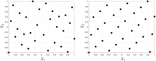
The performance of each OEM is evaluated by taking the RMSE for the other sampling, i.e. for an OEM established for Halton sampling the RMSE is calculated for Hammersley sampling and vice versa. The RMSE for the OEM established for Halton sampling are presented in Table 1, and for the Hammersley sampling the RMSE are given in Table 2. In general, the RMSE are lower for the convex combinations compared to LS and LS-A. Typically, the LS and LS-A have similar values. The LS-C and LST-C have similar values, which, in general, are slightly lower than the values obtained using LSINF-C.

Table 1. RMSE for the five OEMs and all test functions with Halton sampling.

	LS	LS-A	LS-C	LST-C	LSINF-C
$f_1$	0.6938	0.6961	0.6877	0.6906	0.6864
$f_2$	693.76	693.76	693.76	693.76	693.76
$f_3$	23.492	23.839	24.117	23.788	24.398
$f_4$	2.2707	2.2716	2.1806	2.1979	2.2790
$f_5$	0.1376	0.1377	0.1376	0.1376	0.1377
$f_6$	1.7372	1.6899	1.5707	1.5711	1.5717
$f_7$	195.02	193.04	180.95	180.46	180.37
$f_8$	0.7583	0.6959	0.6164	0.6545	0.6531

Table 2. RMSE for the five OEMs and all test functions with Hammersley sampling.

	LS	LS-A	LS-C	LST-C	LSINF-C
$f_1$	0.6946	0.6954	0.6930	0.6935	0.6921
$f_2$	693.76	693.76	693.76	693.76	693.76
$f_3$	30.669	31.860	24.507	24.463	24.597
$f_4$	2.3342	2.3364	2.2341	2.1814	2.5328
$f_5$	0.1376	0.1376	0.1376	0.1376	0.1376
$f_6$	1.3343	1.3357	1.2891	1.3166	1.3831
$f_7$	184.48	185.16	180.141	180.139	180.25
$f_8$	0.7137	0.7243	0.6786	0.6684	0.6850

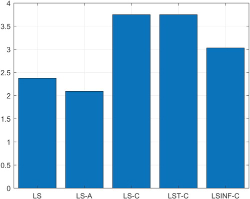
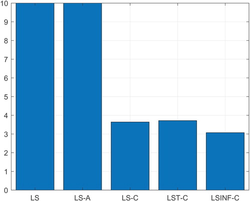
By ranking the OEMs for each test case from 1 (worst) to 5 (best), one obtains the ranking presented in Figure 2. A clear trend is that LS-C and LST-C have a better performance than the other OEMs.

Figure 2. Ranking of the five formulations for establishing the OEMs.

Not only is a better performance obtained using LS-C or LST-C, but also a smoother behaviour of the OEM compared to the behaviour obtained using a linear or affine combination. This difference appears clearly in Figures 3–5, and can be explained by overfitting and the number of metamodels included in the OEM. In general, all 10 metamodels appear in the OEMs of LS and LS-A. For the convex OEMs, three to four metamodels are mostly included in the OEMs. This result is summarized in Figure 6. Thus, automatic pruning of the metamodels is produced by using convex combinations.

Figure 3. The modified Brent test function $f_7$ compared to the OEMs by using LS, LS-A and LS-C. Notice the overfitting for LS and LS-A. (a) $f_7$ in (40(40) $\begin{array}{rl}{f}_1& =\sin \left(4\right(x_1-1)-2)\cos \left(4\right(x_2-1)-2),1\le x_i\le 2,\\ f_2& =100\ast (x_2-x_1^2{)}^2+(x_1-1{)}^2,-2\le x_i\le 2,\\ f_3& =\sqrt{(1000\ast (4/x_1-2{)}^4+1000\ast (4/x_2-2{)}^4)},1\le x_i\le 4,\\ f_4& =\text{peaks}(x_1,x_2),-2\le x_i\le 2,\\ f_5& =\left\{\begin{array}{l}0.6+\sin (16/15\ast x_1-1)+\cdots \\ \sin (16/15\ast x_1-1{)}^2+\cdots \\ \sin (16/15\ast x_2-1)+\cdots \\ \sin (16/15\ast x_2-1{)}^2,\end{array}\right.-1\le x_i\le 1,\\ f_6& =\cos \left(x_1\right)\sin \left(x_2\right)-x_1/(x_2^2+1),-5\le x_i\le 5,\\ f_7& =\left\{\begin{array}{l}(x_1+10{)}^2+(x_2+10{)}^2-\cdots \\ 190\ast \exp (-0.1\ast x_1^2-0.1\ast x_2^2),\end{array}\right.-10\le x_i\le 10,\\ f_8& =\left\{\begin{array}{l}(1-8x_1+7x_1^2-7/3x_1^3+\cdots \\ 1/4x_1^4)x_2^2\exp (-x_2),\end{array}\right.0\le x_i\le 5.\end{array}$(40) )—modified Brent, analytic. (b) $f_7$ in (40(40) $\begin{array}{rl}{f}_1& =\sin \left(4\right(x_1-1)-2)\cos \left(4\right(x_2-1)-2),1\le x_i\le 2,\\ f_2& =100\ast (x_2-x_1^2{)}^2+(x_1-1{)}^2,-2\le x_i\le 2,\\ f_3& =\sqrt{(1000\ast (4/x_1-2{)}^4+1000\ast (4/x_2-2{)}^4)},1\le x_i\le 4,\\ f_4& =\text{peaks}(x_1,x_2),-2\le x_i\le 2,\\ f_5& =\left\{\begin{array}{l}0.6+\sin (16/15\ast x_1-1)+\cdots \\ \sin (16/15\ast x_1-1{)}^2+\cdots \\ \sin (16/15\ast x_2-1)+\cdots \\ \sin (16/15\ast x_2-1{)}^2,\end{array}\right.-1\le x_i\le 1,\\ f_6& =\cos \left(x_1\right)\sin \left(x_2\right)-x_1/(x_2^2+1),-5\le x_i\le 5,\\ f_7& =\left\{\begin{array}{l}(x_1+10{)}^2+(x_2+10{)}^2-\cdots \\ 190\ast \exp (-0.1\ast x_1^2-0.1\ast x_2^2),\end{array}\right.-10\le x_i\le 10,\\ f_8& =\left\{\begin{array}{l}(1-8x_1+7x_1^2-7/3x_1^3+\cdots \\ 1/4x_1^4)x_2^2\exp (-x_2),\end{array}\right.0\le x_i\le 5.\end{array}$(40) )—modified Brent, LS, Halton. (c) $f_7$ in (40(40) $\begin{array}{rl}{f}_1& =\sin \left(4\right(x_1-1)-2)\cos \left(4\right(x_2-1)-2),1\le x_i\le 2,\\ f_2& =100\ast (x_2-x_1^2{)}^2+(x_1-1{)}^2,-2\le x_i\le 2,\\ f_3& =\sqrt{(1000\ast (4/x_1-2{)}^4+1000\ast (4/x_2-2{)}^4)},1\le x_i\le 4,\\ f_4& =\text{peaks}(x_1,x_2),-2\le x_i\le 2,\\ f_5& =\left\{\begin{array}{l}0.6+\sin (16/15\ast x_1-1)+\cdots \\ \sin (16/15\ast x_1-1{)}^2+\cdots \\ \sin (16/15\ast x_2-1)+\cdots \\ \sin (16/15\ast x_2-1{)}^2,\end{array}\right.-1\le x_i\le 1,\\ f_6& =\cos \left(x_1\right)\sin \left(x_2\right)-x_1/(x_2^2+1),-5\le x_i\le 5,\\ f_7& =\left\{\begin{array}{l}(x_1+10{)}^2+(x_2+10{)}^2-\cdots \\ 190\ast \exp (-0.1\ast x_1^2-0.1\ast x_2^2),\end{array}\right.-10\le x_i\le 10,\\ f_8& =\left\{\begin{array}{l}(1-8x_1+7x_1^2-7/3x_1^3+\cdots \\ 1/4x_1^4)x_2^2\exp (-x_2),\end{array}\right.0\le x_i\le 5.\end{array}$(40) )—modified Brent, LS-A, Halton. (d) $f_7$ in (40(40) $\begin{array}{rl}{f}_1& =\sin \left(4\right(x_1-1)-2)\cos \left(4\right(x_2-1)-2),1\le x_i\le 2,\\ f_2& =100\ast (x_2-x_1^2{)}^2+(x_1-1{)}^2,-2\le x_i\le 2,\\ f_3& =\sqrt{(1000\ast (4/x_1-2{)}^4+1000\ast (4/x_2-2{)}^4)},1\le x_i\le 4,\\ f_4& =\text{peaks}(x_1,x_2),-2\le x_i\le 2,\\ f_5& =\left\{\begin{array}{l}0.6+\sin (16/15\ast x_1-1)+\cdots \\ \sin (16/15\ast x_1-1{)}^2+\cdots \\ \sin (16/15\ast x_2-1)+\cdots \\ \sin (16/15\ast x_2-1{)}^2,\end{array}\right.-1\le x_i\le 1,\\ f_6& =\cos \left(x_1\right)\sin \left(x_2\right)-x_1/(x_2^2+1),-5\le x_i\le 5,\\ f_7& =\left\{\begin{array}{l}(x_1+10{)}^2+(x_2+10{)}^2-\cdots \\ 190\ast \exp (-0.1\ast x_1^2-0.1\ast x_2^2),\end{array}\right.-10\le x_i\le 10,\\ f_8& =\left\{\begin{array}{l}(1-8x_1+7x_1^2-7/3x_1^3+\cdots \\ 1/4x_1^4)x_2^2\exp (-x_2),\end{array}\right.0\le x_i\le 5.\end{array}$(40) )—modified Brent, LS-C, Halton.

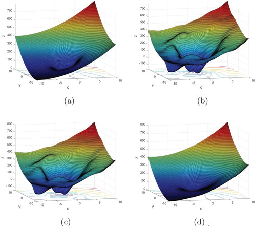
Figure 4. The test function $f_3$ compared to the OEMs by using LS, LS-A and LS-C. Notice the strong overfitting in one of the corners for LS and LS-A. (a) $f_3$ in (40(40) $\begin{array}{rl}{f}_1& =\sin \left(4\right(x_1-1)-2)\cos \left(4\right(x_2-1)-2),1\le x_i\le 2,\\ f_2& =100\ast (x_2-x_1^2{)}^2+(x_1-1{)}^2,-2\le x_i\le 2,\\ f_3& =\sqrt{(1000\ast (4/x_1-2{)}^4+1000\ast (4/x_2-2{)}^4)},1\le x_i\le 4,\\ f_4& =\text{peaks}(x_1,x_2),-2\le x_i\le 2,\\ f_5& =\left\{\begin{array}{l}0.6+\sin (16/15\ast x_1-1)+\cdots \\ \sin (16/15\ast x_1-1{)}^2+\cdots \\ \sin (16/15\ast x_2-1)+\cdots \\ \sin (16/15\ast x_2-1{)}^2,\end{array}\right.-1\le x_i\le 1,\\ f_6& =\cos \left(x_1\right)\sin \left(x_2\right)-x_1/(x_2^2+1),-5\le x_i\le 5,\\ f_7& =\left\{\begin{array}{l}(x_1+10{)}^2+(x_2+10{)}^2-\cdots \\ 190\ast \exp (-0.1\ast x_1^2-0.1\ast x_2^2),\end{array}\right.-10\le x_i\le 10,\\ f_8& =\left\{\begin{array}{l}(1-8x_1+7x_1^2-7/3x_1^3+\cdots \\ 1/4x_1^4)x_2^2\exp (-x_2),\end{array}\right.0\le x_i\le 5.\end{array}$(40) )—analytic. (b) $f_3$ in (40(40) $\begin{array}{rl}{f}_1& =\sin \left(4\right(x_1-1)-2)\cos \left(4\right(x_2-1)-2),1\le x_i\le 2,\\ f_2& =100\ast (x_2-x_1^2{)}^2+(x_1-1{)}^2,-2\le x_i\le 2,\\ f_3& =\sqrt{(1000\ast (4/x_1-2{)}^4+1000\ast (4/x_2-2{)}^4)},1\le x_i\le 4,\\ f_4& =\text{peaks}(x_1,x_2),-2\le x_i\le 2,\\ f_5& =\left\{\begin{array}{l}0.6+\sin (16/15\ast x_1-1)+\cdots \\ \sin (16/15\ast x_1-1{)}^2+\cdots \\ \sin (16/15\ast x_2-1)+\cdots \\ \sin (16/15\ast x_2-1{)}^2,\end{array}\right.-1\le x_i\le 1,\\ f_6& =\cos \left(x_1\right)\sin \left(x_2\right)-x_1/(x_2^2+1),-5\le x_i\le 5,\\ f_7& =\left\{\begin{array}{l}(x_1+10{)}^2+(x_2+10{)}^2-\cdots \\ 190\ast \exp (-0.1\ast x_1^2-0.1\ast x_2^2),\end{array}\right.-10\le x_i\le 10,\\ f_8& =\left\{\begin{array}{l}(1-8x_1+7x_1^2-7/3x_1^3+\cdots \\ 1/4x_1^4)x_2^2\exp (-x_2),\end{array}\right.0\le x_i\le 5.\end{array}$(40) )—LS, Hammersley. (c) $f_3$ in (40(40) $\begin{array}{rl}{f}_1& =\sin \left(4\right(x_1-1)-2)\cos \left(4\right(x_2-1)-2),1\le x_i\le 2,\\ f_2& =100\ast (x_2-x_1^2{)}^2+(x_1-1{)}^2,-2\le x_i\le 2,\\ f_3& =\sqrt{(1000\ast (4/x_1-2{)}^4+1000\ast (4/x_2-2{)}^4)},1\le x_i\le 4,\\ f_4& =\text{peaks}(x_1,x_2),-2\le x_i\le 2,\\ f_5& =\left\{\begin{array}{l}0.6+\sin (16/15\ast x_1-1)+\cdots \\ \sin (16/15\ast x_1-1{)}^2+\cdots \\ \sin (16/15\ast x_2-1)+\cdots \\ \sin (16/15\ast x_2-1{)}^2,\end{array}\right.-1\le x_i\le 1,\\ f_6& =\cos \left(x_1\right)\sin \left(x_2\right)-x_1/(x_2^2+1),-5\le x_i\le 5,\\ f_7& =\left\{\begin{array}{l}(x_1+10{)}^2+(x_2+10{)}^2-\cdots \\ 190\ast \exp (-0.1\ast x_1^2-0.1\ast x_2^2),\end{array}\right.-10\le x_i\le 10,\\ f_8& =\left\{\begin{array}{l}(1-8x_1+7x_1^2-7/3x_1^3+\cdots \\ 1/4x_1^4)x_2^2\exp (-x_2),\end{array}\right.0\le x_i\le 5.\end{array}$(40) )—LS-A, Hammersley. (d) $f_3$ in (40(40) $\begin{array}{rl}{f}_1& =\sin \left(4\right(x_1-1)-2)\cos \left(4\right(x_2-1)-2),1\le x_i\le 2,\\ f_2& =100\ast (x_2-x_1^2{)}^2+(x_1-1{)}^2,-2\le x_i\le 2,\\ f_3& =\sqrt{(1000\ast (4/x_1-2{)}^4+1000\ast (4/x_2-2{)}^4)},1\le x_i\le 4,\\ f_4& =\text{peaks}(x_1,x_2),-2\le x_i\le 2,\\ f_5& =\left\{\begin{array}{l}0.6+\sin (16/15\ast x_1-1)+\cdots \\ \sin (16/15\ast x_1-1{)}^2+\cdots \\ \sin (16/15\ast x_2-1)+\cdots \\ \sin (16/15\ast x_2-1{)}^2,\end{array}\right.-1\le x_i\le 1,\\ f_6& =\cos \left(x_1\right)\sin \left(x_2\right)-x_1/(x_2^2+1),-5\le x_i\le 5,\\ f_7& =\left\{\begin{array}{l}(x_1+10{)}^2+(x_2+10{)}^2-\cdots \\ 190\ast \exp (-0.1\ast x_1^2-0.1\ast x_2^2),\end{array}\right.-10\le x_i\le 10,\\ f_8& =\left\{\begin{array}{l}(1-8x_1+7x_1^2-7/3x_1^3+\cdots \\ 1/4x_1^4)x_2^2\exp (-x_2),\end{array}\right.0\le x_i\le 5.\end{array}$(40) )—LS-C, Hammersley.

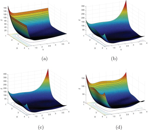
Figure 5. The Hosaki test function $f_8$ compared to the OEMs by using LS, LS-A and LS-C. Notice stronger overfitting along the boundaries for LS and LS-A compared to LS-C. (a) $f_8$ in (40(40) $\begin{array}{rl}{f}_1& =\sin \left(4\right(x_1-1)-2)\cos \left(4\right(x_2-1)-2),1\le x_i\le 2,\\ f_2& =100\ast (x_2-x_1^2{)}^2+(x_1-1{)}^2,-2\le x_i\le 2,\\ f_3& =\sqrt{(1000\ast (4/x_1-2{)}^4+1000\ast (4/x_2-2{)}^4)},1\le x_i\le 4,\\ f_4& =\text{peaks}(x_1,x_2),-2\le x_i\le 2,\\ f_5& =\left\{\begin{array}{l}0.6+\sin (16/15\ast x_1-1)+\cdots \\ \sin (16/15\ast x_1-1{)}^2+\cdots \\ \sin (16/15\ast x_2-1)+\cdots \\ \sin (16/15\ast x_2-1{)}^2,\end{array}\right.-1\le x_i\le 1,\\ f_6& =\cos \left(x_1\right)\sin \left(x_2\right)-x_1/(x_2^2+1),-5\le x_i\le 5,\\ f_7& =\left\{\begin{array}{l}(x_1+10{)}^2+(x_2+10{)}^2-\cdots \\ 190\ast \exp (-0.1\ast x_1^2-0.1\ast x_2^2),\end{array}\right.-10\le x_i\le 10,\\ f_8& =\left\{\begin{array}{l}(1-8x_1+7x_1^2-7/3x_1^3+\cdots \\ 1/4x_1^4)x_2^2\exp (-x_2),\end{array}\right.0\le x_i\le 5.\end{array}$(40) )—Hosaki, analytic. (b) $f_8$ in (40(40) $\begin{array}{rl}{f}_1& =\sin \left(4\right(x_1-1)-2)\cos \left(4\right(x_2-1)-2),1\le x_i\le 2,\\ f_2& =100\ast (x_2-x_1^2{)}^2+(x_1-1{)}^2,-2\le x_i\le 2,\\ f_3& =\sqrt{(1000\ast (4/x_1-2{)}^4+1000\ast (4/x_2-2{)}^4)},1\le x_i\le 4,\\ f_4& =\text{peaks}(x_1,x_2),-2\le x_i\le 2,\\ f_5& =\left\{\begin{array}{l}0.6+\sin (16/15\ast x_1-1)+\cdots \\ \sin (16/15\ast x_1-1{)}^2+\cdots \\ \sin (16/15\ast x_2-1)+\cdots \\ \sin (16/15\ast x_2-1{)}^2,\end{array}\right.-1\le x_i\le 1,\\ f_6& =\cos \left(x_1\right)\sin \left(x_2\right)-x_1/(x_2^2+1),-5\le x_i\le 5,\\ f_7& =\left\{\begin{array}{l}(x_1+10{)}^2+(x_2+10{)}^2-\cdots \\ 190\ast \exp (-0.1\ast x_1^2-0.1\ast x_2^2),\end{array}\right.-10\le x_i\le 10,\\ f_8& =\left\{\begin{array}{l}(1-8x_1+7x_1^2-7/3x_1^3+\cdots \\ 1/4x_1^4)x_2^2\exp (-x_2),\end{array}\right.0\le x_i\le 5.\end{array}$(40) )—Hosaki, LS, Halton. (c) $f_8$ in (40(40) $\begin{array}{rl}{f}_1& =\sin \left(4\right(x_1-1)-2)\cos \left(4\right(x_2-1)-2),1\le x_i\le 2,\\ f_2& =100\ast (x_2-x_1^2{)}^2+(x_1-1{)}^2,-2\le x_i\le 2,\\ f_3& =\sqrt{(1000\ast (4/x_1-2{)}^4+1000\ast (4/x_2-2{)}^4)},1\le x_i\le 4,\\ f_4& =\text{peaks}(x_1,x_2),-2\le x_i\le 2,\\ f_5& =\left\{\begin{array}{l}0.6+\sin (16/15\ast x_1-1)+\cdots \\ \sin (16/15\ast x_1-1{)}^2+\cdots \\ \sin (16/15\ast x_2-1)+\cdots \\ \sin (16/15\ast x_2-1{)}^2,\end{array}\right.-1\le x_i\le 1,\\ f_6& =\cos \left(x_1\right)\sin \left(x_2\right)-x_1/(x_2^2+1),-5\le x_i\le 5,\\ f_7& =\left\{\begin{array}{l}(x_1+10{)}^2+(x_2+10{)}^2-\cdots \\ 190\ast \exp (-0.1\ast x_1^2-0.1\ast x_2^2),\end{array}\right.-10\le x_i\le 10,\\ f_8& =\left\{\begin{array}{l}(1-8x_1+7x_1^2-7/3x_1^3+\cdots \\ 1/4x_1^4)x_2^2\exp (-x_2),\end{array}\right.0\le x_i\le 5.\end{array}$(40) )—Hosaki, LS-A, Halton. (d) $f_8$ in (40(40) $\begin{array}{rl}{f}_1& =\sin \left(4\right(x_1-1)-2)\cos \left(4\right(x_2-1)-2),1\le x_i\le 2,\\ f_2& =100\ast (x_2-x_1^2{)}^2+(x_1-1{)}^2,-2\le x_i\le 2,\\ f_3& =\sqrt{(1000\ast (4/x_1-2{)}^4+1000\ast (4/x_2-2{)}^4)},1\le x_i\le 4,\\ f_4& =\text{peaks}(x_1,x_2),-2\le x_i\le 2,\\ f_5& =\left\{\begin{array}{l}0.6+\sin (16/15\ast x_1-1)+\cdots \\ \sin (16/15\ast x_1-1{)}^2+\cdots \\ \sin (16/15\ast x_2-1)+\cdots \\ \sin (16/15\ast x_2-1{)}^2,\end{array}\right.-1\le x_i\le 1,\\ f_6& =\cos \left(x_1\right)\sin \left(x_2\right)-x_1/(x_2^2+1),-5\le x_i\le 5,\\ f_7& =\left\{\begin{array}{l}(x_1+10{)}^2+(x_2+10{)}^2-\cdots \\ 190\ast \exp (-0.1\ast x_1^2-0.1\ast x_2^2),\end{array}\right.-10\le x_i\le 10,\\ f_8& =\left\{\begin{array}{l}(1-8x_1+7x_1^2-7/3x_1^3+\cdots \\ 1/4x_1^4)x_2^2\exp (-x_2),\end{array}\right.0\le x_i\le 5.\end{array}$(40) )—Hosaki, LS-C, Halton.

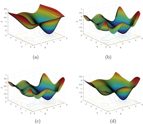
Figure 6. The number of metamodels on average for the OEMs by using the five different formulations.

LS and LS-A also suffer from overfitting. Frequently, a large positive weight is cancelled out by a large negative value on another weight, see for example the optimal weights for the modified Brent test function in Table 3 and the plots in Figure 3. In this particular test example, the performances of the convex combinations are superior over the performances of the linear and affine combinations. This can be concluded by studying the plots in Figure 3.

Table 3. The optimal weights for the modified Brent test function $f_7$. Notice the pruning obtained using LS-C, LST-C and LSINF-C, as well as the appearance of large positive and negative weights cancelling out each other for the LS and LS-A.

		LS	LS-A	LS-C	LST-C	LSINF-C
Halton sampling	Q	$-1.1028$	$-0.9550$	0	0	0
	Kr-L	5.4626	4.2695	0	0.1624	0
	Kr-Q	$-46.4788$	$-44.7000$	0	0	0
	Rpri-L	1.5266	2.4328	0	0	0
	Rpri-Q	9.4921	7.8856	0	0.8206	0
	Rpost-L	$-6.9526$	$-6.8063$	0	0	0
	Rpost-Q	38.8747	38.6706	0.9629		0.8981
	PCE	0.0957	0.1095	0.0339	0.0170	0.1019
	SVR	$-134.0466$	$-59.2279$	0	0	0
	L-SVR	134.1011	59.3213	0.0032	0	0
Hammersley sampling	Q	$-0.4607$	$-0.4864$	0	0	0
	Kr-L	2.6953	3.3076	0.2057	0.1998	0
	Kr-Q	$-0.1840$	$-1.1752$	0.7943	0.8002	0.9645
	Rpri-L	$-1.2439$	$-0.3428$	0	0	0
	Rpri-Q	$-1.8412$	$-1.1152$	0	0	0
	Rpost-L	$-1.3765$	$-2.8381$	0	0	0
	Rpost-Q	3.4171	3.6560	0	0	0
	PCE	$-0.0131$	$-0.0141$	0	0	0.0355
	SVR	$-63.9897$	$-34.1317$	0	0	0
	L-SVR	63.9771	34.1399	0	0	0

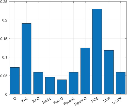
Although automatic pruning is generated using convex combinations, all metamodels appear sometimes in the convex OEMs, see Figure 7. From this figure one can also see that Kriging-L and PCE are the real workhorses for the examples studied in this article, but also Rpost-Q and SVR appear more frequently than the others.

Figure 7. The frequency of metamodels appearing in the ensemble for LS-C, LST-C and LSINF-C.

Finally, a most established design optimization benchmark is solved using optimal affine (LS-A) and convex (LST-C) combinations of metamodels. The welded beam problem considered by Garg (2014) and Amouzgar and Strömberg (2017) is studied. The governing equations of the problem read (41) $\left\{\begin{array}{l}\underset{x_i}{min}f=1.104,71x_1^2{x}_2+0.048,11x_3{x}_4(14+x_2)\\ \text{s.t. }\left\{\begin{array}{l}{g}_1=\tau \left(x_i\right)-\mathrm{13,600}\le 0,\\ g_2=\sigma \left(x_i\right)-\mathrm{30,000}\le 0,\\ g_3=x_1-x_4\le 0,\\ g_4=0.125-x_1\le 0,\\ g_5=\delta \left(x_i\right)-0.25\le 0,\\ g_6=\mathrm{6,000}-P_c\left(x_i\right)\le 0,\end{array}\right.\end{array}\right.$(41) where the definitions of the shear stress $\tau \left(x_i\right)$, normal stress $\sigma \left(x_i\right)$, displacement $\delta \left(x_i\right)$ and critical force $P_c\left(x_i\right)$ can be found in Amouzgar and Strömberg (2017). In addition, the variables are bounded by $0.1\le x_1,$ $x_4\le 2$ and $0.1\le x_2,$ $x_3\le 10$. The optimal solution obtained by GA and SLP is $(0.24437,6.2175,8.2915,0.24437)$. An almost identical solution was presented by Garg (2014). In Amouzgar and Strömberg (2017), this benchmark was solved using screening with a total number of 60 sampling points and radial basis function networks. The solution obtained in their work was (0.4147, 3.926, 6.6201, 0.4147), which violated the first constraint.

In this work, the problem is solved by setting up Halton sampling using 60 points without any screening and establishing optimal affine (LS-A by solving 10(10) $\mathit{w}=\frac{{\mathit{C}}^{-1}\mathbf{1}}{{\mathbf{1}}^{\mathrm{T}}{\mathit{C}}^{-1}\mathbf{1}},$(10) ) and convex combinations (LST-C) of the following metamodels: Q, Kr-L, Rpri-Q, Rpost-Q, SVR and L-SVR. The optimal weights for LS-A by solving (10(10) $\mathit{w}=\frac{{\mathit{C}}^{-1}\mathbf{1}}{{\mathbf{1}}^{\mathrm{T}}{\mathit{C}}^{-1}\mathbf{1}},$(10) ) are presented in Table 4 and the optimal weights for LST-C by solving (17(17) $\text{(LST-C)}\left\{\begin{array}{l}\underset{(\mathit{w},\mathit{p},\mathit{q})}{min}\sum _{i=1}^N{p}_i+q_i\\ \text{s.t. }\left\{\begin{array}{l}\mathit{Y}\mathit{w}-\hat{\mathit{f}}=\mathit{p}-\mathit{q},\\ {\mathit{w}}^{\mathrm{T}}\mathbf{1}=1,\\ w_i,p_j,q_j\ge 0,i=1,\dots ,M,j=1,\dots ,N.\end{array}\right.\end{array}\right.$(17) ) are presented in Table 5. The pruning effect using LST-C appears clearly when compared to the solution for LS-A, where no pruning is obtained. The drawback with large positive weights cancelled out by large negative weights using LS-A appears for f and $g_5$ in Table 4.

Table 4. The optimal weights for the affine combination (LS-A) defined by (10(10) $\mathit{w}=\frac{{\mathit{C}}^{-1}\mathbf{1}}{{\mathbf{1}}^{\mathrm{T}}{\mathit{C}}^{-1}\mathbf{1}},$(10) ). No pruning is observed.

	Q	Kr-L	Rpri-Q	Rpost-Q	SVR	L-SVR
f	$0.132539$	$0.051347$	$0.215711$	$0.616404$	$-56.608$	$56.59241$
$g_1$	$-0.00319$	$-0.00074$	$-0.00905$	$0.076107$	$0.98712$	$-0.05025$
$g_2$	$-0.00468$	$0.120128$	$-0.15153$	$0.391141$	$0.925492$	$-0.28055$
$g_3$	$0.929655$	$0.228807$	$-0.29217$	$0.133712$	$-2.5\mathrm{E}-05$	$2.45\mathrm{E}-05$
$g_4$	$-0.00289$	$1.020569$	$0.002164$	$-0.01984$	$-1.3\mathrm{E}-13$	$1.28\mathrm{E}-13$
$g_5$	$0.13262$1	$0.441647$	$0.017628$	$0.474479$	$5.17683$	$-5.2432$
$g_6$	$1.521595$	$-0.04111$	$0.218327$	$-0.87672$	$-0.01469$	$0.19259$

Table 5. The optimal weights for the convex combination (LST-C) defined by (17(17) $\text{(LST-C)}\left\{\begin{array}{l}\underset{(\mathit{w},\mathit{p},\mathit{q})}{min}\sum _{i=1}^N{p}_i+q_i\\ \text{s.t. }\left\{\begin{array}{l}\mathit{Y}\mathit{w}-\hat{\mathit{f}}=\mathit{p}-\mathit{q},\\ {\mathit{w}}^{\mathrm{T}}\mathbf{1}=1,\\ w_i,p_j,q_j\ge 0,i=1,\dots ,M,j=1,\dots ,N.\end{array}\right.\end{array}\right.$(17) ). The pruning effect appears clearly.

	Q	Kr-L	Rpri-Q	Rpost-Q	SVR	L-SVR
f	0.047168	0.007572	0.411331	0.405335	0	0.128595
$g_1$	0	0.001568	0	0.002536	0.995896	0
$g_2$	0.001524	0.003445	0	0	0.99503	0
$g_3$	1	0	0	0	0	0
$g_4$	0	0	0	1	0	0
$g_5$	0.067295	0.336798	0	0.089569	0.506338	0
$g_6$	0.835986	0.023852	0	0	0.060372	0.07979

In Table 6, the optimal solutions for all metamodels as well as the affine and convex combinations of metamodels are presented. By just studying the objective value f, one obtains the following ranking: Rpri-Q, L-SVR, Rpost-Q, Kr-L, LS-A, Q, LST-C and SVR. It might seem that the performance of LST-C and SVR are poor. However, by studying the corresponding constraints values in Table 7, one realizes that only the optimal solutions obtained using LST-C and SVR are feasible. All the other metamodels fail; also the affine combination LS-A fails. Thus, the best performance is obtained using LST-C, which in turn is much better than the performance obtained using SVR.

Table 6. The optimal solution using LS-A and LST-C as well as the metamodels of the ensemble taken separately.

	$x_1$	$x_2$	$x_3$	$x_4$	f
Q	0.125	10	2.457013	1.25005	3.71896
Kr-L	0.125	7.158803	2.099708	0.701041	1.621972
Rpri-Q	0.190296	2.726508	0.490942	1.307938	0.625796
Rpost-Q	0.488229	3.348341	0.1	1.367993	0.995885
SVR	0.617535	2.672035	7.724021	1.922396	13.03564
L-SVR	0.1	2.836651	1.71804	0.458387	0.669243
LS-A (10(10) $\mathit{w}=\frac{{\mathit{C}}^{-1}\mathbf{1}}{{\mathbf{1}}^{\mathrm{T}}{\mathit{C}}^{-1}\mathbf{1}},$(10) )	0.962134	0.337418	2.763382	1.043308	2.333711
LST-C	0.675136	3.242391	5.931528	0.81185	5.627279

Table 7. The corresponding constraint values for the optimal solutions presented in Table 6. Negative values are feasible.

	$g_1$	$g_2$	$g_3$	$g_4$	$g_5$	$g_6$
Q	$22997.62$	$36786.43$	$-1.12505$	0	$-0.13161$	$-283187$
Kr-L	$47661.98$	$133068.2$	$-0.57604$	0	$0.088263$	$-38061.6$
Rpri-Q	$234347.1$	$1568759$	$-1.11764$	$-0.0653$	$13.93392$	$-64136.3$
Rpost-Q	$56695.68$	$36812294$	$-0.87976$	$-0.36323$	$1604.437$	$-10528.6$
SVR	$-2931.67$	$-25605.6$	$-1.30486$	$-0.49254$	$-0.24752$	$-2772080$
L-SVR	$258642.1$	$342504.7$	$-0.35839$	0.025	$0.69437$	$-4194.09$
LS-A (10(10) $\mathit{w}=\frac{{\mathit{C}}^{-1}\mathbf{1}}{{\mathbf{1}}^{\mathrm{T}}{\mathit{C}}^{-1}\mathbf{1}},$(10) )	$87955.54$	$33261.01$	$-0.08117$	$-0.83713$	$-0.15029$	$-181332$
LST-C	$-3149.56$	$-12355$	$-0.13671$	$-0.55014$	$-0.23704$	$-165082$

5. Concluding remarks

In this article, a general framework for generating optimal linear, affine and convex combinations of metamodels by minimizing the PRESS using the taxicab, Euclidean or infinity norm are presented and studied. Thus, the formulation proposed by Viana, Haftka, and Steffen (2009) is not the starting point in this article, but instead derived symbolically as a special case for affine combinations using the Euclidean norm. It is concluded from the study that convex combinations are preferable over linear as well as the established affine combinations. The risk of overfitting is less and automatic pruning of metamodels is obtained. In conclusion, it is suggested that the optimal weights of the convex combinations of metamodels be established by minimizing the Euclidean norm or the taxicab norm of the residual vector of the leave-one-out cross-validation errors, where the former formulation implies a QP-problem and the latter one is an LP-problem to be solved. For future work, it is suggested to study the performance of these two formulations for large problems, in order to establish if the QP-problem is preferable over the LP-problem or vice versa.

Disclosure statement

No potential conflict of interest was reported by the author(s).

ORCID

Niclas Strömberg  http://orcid.org/0000-0001-6821-5727

Notes

1 MetaBox, http://www.fema.se

2 The optimal weights for the OEMs for all test functions in (40(40) $\begin{array}{rl}{f}_1& =\sin \left(4\right(x_1-1)-2)\cos \left(4\right(x_2-1)-2),1\le x_i\le 2,\\ f_2& =100\ast (x_2-x_1^2{)}^2+(x_1-1{)}^2,-2\le x_i\le 2,\\ f_3& =\sqrt{(1000\ast (4/x_1-2{)}^4+1000\ast (4/x_2-2{)}^4)},1\le x_i\le 4,\\ f_4& =\text{peaks}(x_1,x_2),-2\le x_i\le 2,\\ f_5& =\left\{\begin{array}{l}0.6+\sin (16/15\ast x_1-1)+\cdots \\ \sin (16/15\ast x_1-1{)}^2+\cdots \\ \sin (16/15\ast x_2-1)+\cdots \\ \sin (16/15\ast x_2-1{)}^2,\end{array}\right.-1\le x_i\le 1,\\ f_6& =\cos \left(x_1\right)\sin \left(x_2\right)-x_1/(x_2^2+1),-5\le x_i\le 5,\\ f_7& =\left\{\begin{array}{l}(x_1+10{)}^2+(x_2+10{)}^2-\cdots \\ 190\ast \exp (-0.1\ast x_1^2-0.1\ast x_2^2),\end{array}\right.-10\le x_i\le 10,\\ f_8& =\left\{\begin{array}{l}(1-8x_1+7x_1^2-7/3x_1^3+\cdots \\ 1/4x_1^4)x_2^2\exp (-x_2),\end{array}\right.0\le x_i\le 5.\end{array}$(40) ) can be obtained from the author upon request by sending an e-mail to [email protected]

Appendix 1. Symbolic proof

Below, in this appendix, the MATLAB${}^{\text{®}}$ code for a symbolic proof showing that the optimal weights for an affine combination by minimizing the PRESS in (8(8) $\mathit{w}=({\mathit{Y}}^{\mathrm{T}}\mathit{Y}{)}^{-1}\left({\mathit{Y}}^{\mathrm{T}}\hat{\mathit{f}}-\lambda \mathbf{1}\right),$(8) ) and (9(9) $\lambda =\frac{{\mathbf{1}}^{\mathrm{T}}({\mathit{Y}}^{\mathrm{T}}\mathit{Y}{)}^{-1}{\mathit{Y}}^{\mathrm{T}}\hat{\mathit{f}}-1}{{\mathbf{1}}^{\mathrm{T}}({\mathit{Y}}^{\mathrm{T}}\mathit{Y}{)}^{-1}\mathbf{1}}.$(9) ) are identical to the optimal weights (10(10) $\mathit{w}=\frac{{\mathit{C}}^{-1}\mathbf{1}}{{\mathbf{1}}^{\mathrm{T}}{\mathit{C}}^{-1}\mathbf{1}},$(10) ) by using the formulation by Viana, Haftka, and Steffen (2009) is given.

References

- Acar, E. 2010. “Various Approaches for Constructing An Ensemble of Metamodels Using Local Measures.” Structural and Multidisciplinary Optimization 42: 879–896. doi:10.1007/s00158-010-0520-z
- Acar, E., and M. Rais-Rohani. 2009. “Ensemble of Metamodels with Optimized Weight Factors.” Structural and Multidisciplinary Optimization 37: 279–294. doi:10.1007/s00158-008-0230-y
- Amouzgar, K., A. Rashid, and N. Strömberg. 2013. “Multi-Objective Optimization of a Disc Brake System by Using SPEA2 and RBFN.” In Proceedings of the 39th Design Automation Conference. New York: ASME.
- Amouzgar, K., and N. Strömberg. 2017. “Radial Basis Functions As Surrogate Models with a Priori Bias in Comparison with a Posteriori Bias.” Structural and Multidisciplinary Optimization 55: 1453–1469. doi:10.1007/s00158-016-1569-0
- Breiman, L. 1996. “Stacked Regressions.” Machine Learning 24: 49–64. doi:10.1007/BF00117832
- Ferreira, W. G., and A. L. Serpa. 2016. “Ensemble of Metamodels: The Augmented Least Squares Approach.” Structural and Multidisciplinary Optimization 53: 1019–1046. doi:10.1007/s00158-015-1366-1
- Garg, H. 2014. “Solving Structural Engineering Design Optimization Problems Using An Artificial Bee Colony Algorithm.” Journal of Industrial and Management Optimization 10 (3): 777–794. doi:10.3934/jimo.2014.10.777
- Goel, T., R. T. Haftka, W. Shyy, and N. V. Queipo. 2007. “Ensemble of Surrogates.” Structural and Multidisciplinary Optimization 33: 199–216. doi:10.1007/s00158-006-0051-9
- Kleijnen, J. P. C. 2009. “Kriging Metamodeling in Simulation: A Review.” European Journal of Operational Research 192 (3): 707–716. doi:10.1016/j.ejor.2007.10.013
- Lee, Y., and D.-H. Choi. 2014. “Pointwise Ensemble of Meta-Models Using ν Nearest Points Cross-Validation.” Structural and Multidisciplinary Optimization 50: 383–394. doi:10.1007/s00158-014-1067-1
- Shi, R., L. Liu, T. Long, and J. Liu. 2016. “An Efficient Ensemble of Radial Basis Functions Method Based on Quadratic Programming.” Engineering Optimization 48: 1202–1225. doi:10.1080/0305215X.2015.1100470
- Song, X., L. Lv, J. Li, W. Sun, and J. Zhang. 2018. “An Advanced and Robust Ensemble Surrogate Model: Extended Adaptive Hybrid Functions.” Journal of Mechanical Design 140 (4): Article ID 041402. doi:10.1115/1.4039128
- Strömberg, N. 2016. “Reliability-Based Design Optimization by Using a SLP Approach and Radial Basis Function Networks.” In Proceedings of the 2016 International Design Engineering Technical Conferences & Computers and Information in Engineering Conference (IDETC/CIE). New York: ASME.
- Strömberg, N. 2018a. “Reliability-Based Design Optimization by Using Support Vector Machines.” In Proceedings of ESREL—the European Safety and Reliability Conference. London: CRC Press. doi:10.1201/9781351174664.
- Strömberg, N. 2018b. “Reliability-Based Design Optimization by Using Metamodels.” In Proceedings of the 6th International Conference on Engineering Optimization (EngOpt 2018). Cham, Switzerland: Springer International Publishing. doi:10.1007/978-3-319-97773-7.
- Strömberg, N. 2019. “Reliability-Based Design Optimization by Using Ensemble of Metamodels.” In Proceedings of the 3rd International Conference on Uncertainty Quantification in Computational Sciences and Engineering (UNCECOMP 2019). Athens: UNDECOMP.
- Strömberg, N., and M. Tapankov. 2012. “Sampling- and SORM-based RBDO of a Knuckle Component by Using Optimal Regression Models.” In Proceedings of the 14th AIAA/ISSMO Multidisciplinary Analysis and Optimization Conference. Reston, VA: AIAA. doi:10.2514/6.2012-5439.
- Sudret, B. 2008. “Global Sensitivity Analysis Using Polynomial Chaos Expansions.” Reliability Engineering & System Safety 93 (7): 964–979. doi:10.1016/j.ress.2007.04.002
- Viana, F. A. C., R. T. Haftka, and V. Steffen Jr. 2009. “Multiple Surrogates: How Cross-Validation Errors Can Help Us to Obtain the Best Predictor.” Structural and Multidisciplinary Optimization 39: 439–457. doi:10.1007/s00158-008-0338-0
- Wang, G. G., and S. Shan. 2006. “Review of Metamodeling Techniques in Support of Engineering Design Optimization.” Journal of Mechanical Design 129 (4): 370–380. doi:10.1115/1.2429697
- Wolpert, D. H. 1992. “Stacked Generalization.” Neural Networks 5: 241–259. doi:10.1016/S0893-6080(05)80023-1
- Xiao, Jian Zhou, Zhong Ma Yi, and Fang Li Xu. 2011. “Ensembles of Surrogates with Recursive Arithmetic Average.” Structural and Multidisciplinary Optimization 44: 651–671. doi:10.1007/s00158-011-0655-6 doi: 10.1007/s00158-011-0652-9
- Yun, Y., M. Yoon, and H. Nakayama. 2009. “Multi-Objective Optimization Based on Meta-modeling by Using Support Vector Regression.” Optimization and Engineering 10: 167–181. doi:10.1007/s11081-008-9063-1
- Zhou, Z.-H. 2012. Ensemble Methods, Foundations and Algorithms. New York: Chapman and Hall/CRC. doi:10.1201/b12207