Improved NEH-based heuristic for the blocking flow-shop problem with bicriteria of the makespan and machine utilization

Abstract

The blocking flow-shop scheduling problem, which is an NP-hard problem, has wide applications in industry. Many studies have focused primarily on single-objective optimization, such as minimizing the makespan or total flow time, which is insufficient for practical problems. In this study, a blocking flow-shop scheduling problem with bicriteria of the makespan and machine utilization is considered. A simple constructive heuristic, NEHCG, is proposed by developing new priority and tie-breaking rules based on the Nawaz–Enscore–Ham heuristic. In the new priority rule, the quartile deviation of job processing times is included for the first time, and the new tie-breaking rule is designed to break ties effectively in the insertion phase. Then, an improved constructive heuristic, PW_NEHCG, is presented by effectively combining NEHCG with an improved profile-fitting approach. Computational experiments show that the proposed constructive heuristics exhibit excellent performance compared to other well-known heuristics.

KEYWORDS:

• Heuristic
• blocking flow shop
• makespan
• idle time
• blocking time

1. Introduction

The permutation flow-shop scheduling problem (PFSP) is a common industrial production layout problem (Yenisey and Yagmahan 2014). Machines are located according to a fixed order with unlimited buffers between successive machines and jobs are processed consecutively on the line. However, in a practical production environment, the work in process must be minimized to save capital investment, and the buffers between machines are set to zero; this is denoted by the blocking flow-shop scheduling problem (BFSP). This problem is applicable to many industries, such as the chemical and pharmaceutical industries, just-in-time production lines and robotic cells (Miyata and Nagano 2019). However, the problem of blocking constraints in the BFSP deserves more attention.

For the BFSP, three well-known constraints have been developed: the classical release when starting blocking (RSb) constraint, the special release when completing blocking (RCb) constraint and the special RCb* constraint (Riahi et al. 2017). The RCb* constraint is a variant of the RCb constraint which is widely observed in cider production plants (Trabelsi, Sauvey, and Sauer 2012). It supposes that machine $j$ cannot start processing job $i+1$ until machine $j+1$ completes the job. A discussion of these constraints is available at https://doi.org/10.6084/m9.figshare.16908529.

A large amount of effort has been put into the BFSP with RCb* constraints. Trabelsi, Sauvey, and Sauer (2012) proposed a mathematical model of the mixed BFSP under the without blocking (WB), RSb, RCb and RCb* constraints, and presented the TSS heuristic to minimize the makespan. Riahi et al. (2019) proposed a constructive search approach and a constraint-guided local search (CGLS). Lin et al. (2021) developed an improved degradation algorithm for multi-temperature simulations, which is superior to CGLS. However, these studies only considered BFSP with RCb* in the case of a single criterion, which is not sufficient to describe complex practical problems. In view of the importance of multi-objective BFSP and the relative lack of research in this area, it is essential to investigate the multi-objective BFSP with the RCb* constraint.

The BFSP with RCb* has been shown to be NP hard for more than three machines by Trabelsi, Sauvey, and Sauer (2012), and heuristic approaches have commonly been investigated for solving large-size BFSPs. The Nawaz–Enscore–Ham (NEH) heuristic has proven to be the most efficient heuristic for makespan minimization in the PFSP (Nawaz, Emory Enscore, and Ham 1983). Framinan, Leisten, and Rajendran (2003) constructed 177 different priority rules. However, their results demonstrated that the NEH heuristic perform best with the makespan objective. For the same objective, Wang, Pan, and Fatih Tasgetiren (2010) introduced NEH_WPT for the BFSP. Riahi et al. (2017) proposed NNEH with a new initial order for solving the mixed BFSP. Dong, Huang, and Chen (2008) developed NEH_D, which added the standard deviation to the priority rule, and proposed a tie-breaking rule to balance machine utilization. Kalczynski and Kamburowski (2008, 2009) proposed a weighted process time method based on Johnson’s algorithm and devised the NEHKK1 and NEHKK2 algorithms. For the bicriteria of the makespan and idle time, Liu, Jin, and Price (2016) introduced new priority and tie-breaking rules and developed the NEHLJP algorithm.

The combination of the profile-fitting (PF) approach and the NEH insertion procedure has been demonstrated to be effective. To solve the BFSP with the makespan objective, McCormick et al. (1989) introduced the PF heuristic. Ronconi (2004) established the MinMax (MM), MME and PFE algorithms based on the NEH heuristic, where the initial order is generated by the MM and PF heuristics. Pan and Wang (2012) suggested an effective method to combine the PF with the NEH heuristics, and proposed PF_NEH($x$), WPF_NEH($x$) and PW_NEH($x$). Tasgetiren et al. (2017) proposed PFT_NEH($x$) by improving the cost function for selecting the next job based on PF_NEH($x$). To solve the BFSP with the total flow time objective, Ribas and Companys (2015) proposed the NHPF1 and NHPF2 heuristics. Tasgetiren et al. (2016) presented the tPF_NEH ($x$) heuristic.

In this article, machine utilization and makespan are comprehensively evaluated when solving the BFSP under the RCb* constraint. Heuristic algorithms based on the NEH method are presented to solve the problem. Comparisons are performed and the effectiveness of the proposed heuristics is verified.

The remainder of this article is organized as follows. Section 2 investigates related work. Section 3 describes the issues relevant to the research. Section 4 provides a detailed description of the proposed heuristic algorithms. Section 5 describes the cases tested, presents computational results and assesses the effectiveness of the proposed algorithms. Section 6 concludes the article.

2. Related work

The BFSP has attracted considerable attention in recent years. Based on the objective function, BFSPs can be divided into single-objective optimization problems and multi-objective optimization problems. Studies related to these two aspects of the BFSP are briefly reviewed in this section.

Most previous research focused on single-objective optimization problems, among which the most widely studied objective function is the makespan. Wang et al. (2010) developed a hybrid discrete differential evolution algorithm and an acceleration method to improve the algorithm efficiency. Lebbar et al. (2018) proposed two evolutionary optimization methods, including a genetic algorithm and the simulated annealing genetic algorithm. Fewer studies have concentrated on the other objectives. For the flow time, Shao, Pi, and Shao (2017) presented a self-adaptive discrete invasive weed optimization and improved the best known solutions for 132 out of 480 problem instances. Robazzi, Nagano, and Takano (2021) studied a PFSP with blocking and set-up times and proposed an improved branch-and-bound algorithm. For the total tardiness, Ribas, Companys, and Tort-Martorell (2013) integrated the iterated local search and variable neighbourhood search procedures. Nagano, Komesu, and Miyata (2019) developed an algorithm combining evolutionary clustering search and variable neighbourhood search. For the total completion time criterion, Nagano, Robazzi, and Tomazella (2020) presented a new lower-bound algorithm considering both machine idleness and the occurrence of blocking.

Studies on the multi-objective BFSP have increased in recent years. For the makespan and total flow time, Deng et al. (2016) proposed a multi-objective discrete differential evolution algorithm. Shao, Pi, and Shao (2019) constructed a novel multi-objective discrete water wave optimization algorithm. For the makespan and total completion time, Nouri and Ladhari (2018) developed a genetic algorithm (MBGA) based on the non-dominated sorting genetic algorithm II (NSGA-II). To minimize the weighted sum of the total tardiness and makespan, Lebbar, Barkany, and Jabri (2017) proposed a new mixed-integer linear programming (MILP) model to solve multi-machine flow-shop scheduling problems with finite buffers and different release dates of job constraints. For the bicriteria optimization of the same objectives, Aqil and Allali (2021) presented a MILP method and a set of different metaheuristics. For the total energy consumption and makespan, Han et al. (2020) proposed a discrete evolutionary multi-objective optimization algorithm to solve the multi-objective BFSP with set-up time.

In general, metaheuristic methods require more computational effort to obtain a better solution than heuristic methods, which makes it difficult to meet the requirements of practical applications, especially for large-scale problems (Li, Wang, and Wu 2009). Therefore, heuristic algorithms are crucial for manufacturing systems because they can find good solutions in a reasonable time, which is the main motivation of this study.

3. Problem description

3.1. BFSP

The BFSP can be described as follows. There are $n$ jobs from the set $J=\{1,2,\dots ,n\}$ and $m$ machines from the set $M=\{1,2,\dots ,m\}$. Each job, $j\in J$, is processed sequentially on machines $1,2,\dots ,m$. The processing time of process $i$ on machine $j$ is expressed as $T_{i,j}$. This study considers a BFSP with an RCb* constraint. There are no intermediate buffers between two machines, such that machine $j$ cannot process job $i+1$ until machine $j+1$ completes job $i$. In this study, machines $1,\dots m-1$ are subject to the RCb* constraint, while the last machine always operates under the Wb constraint, denoted by (1) $\begin{array}{rl}{B}_k& =RCb\ast ,k=1,\dots ,m-1\end{array}$(1) (2) $\begin{array}{rl}{B}_m& =Wb\end{array}$(2) where $B_k$ denotes the blocking constraint condition of the kth machine.

Table 1 defines the notations used in this article.

Table 1 Notation definitions.

Parameter	Definition
N	Total number of jobs
M	Total number of machines
I	Index for job, 1 ≤ i ≤ n
K	Index for machine, 1 ≤ k ≤ m
Π	Permutation of the given n jobs
$T_{[i],k}$	Process time of the ith job of permutation π on machine k
$I{T}_{[i],k}$	Idle time of machine k generated by the ith job of permutation π
$B{T}_{[i],k}$	Blocking time of machine k generated by the ith job of permutation π
$S_{[i],k}$	Starting time of the ith job of permutation π on machine k
$C_{[i],k}$	Completion time of the ith job of permutation π on machine k
$d_{[i],k}$	Departure time of the ith job of permutation π on machine k

For the BFSP, the following assumptions are made:

1. Each job is processed at most once on each machine.

2. A machine cannot process two or more jobs simultaneously.

3. A job cannot be processed on two or more machines simultaneously.

4. Pre-emption of operations is forbidden.

5. The buffer capacity between any two successive machines is zero.

3.2. Bicriteria BFSP

The non-processing time can be divided into the front delay, idle time, blocking time and back delay, as shown at https://doi.org/10.6084/m9.figshare.16908529 (Spachis 1979). In a continuous production environment, the front delay can be taken up by previous operations and the back delay can be used by subsequent tasks; therefore, the idle time and blocking time represent the real wasted time and can be used as indicators of production system efficiency. The maximization of machine utilization can thus be expressed as the minimization of the blocking time and idle time (Liu, Jin, and Price 2016; Maassena, Perez-Gonzalez, and Gunther 2020). Hence, the bicriteria of the makespan and machine utilization can be formulated as follows: (3) $\begin{array}{r}F=min\{C_{max},(BT,IT)\}\end{array}$(3) where $C_{max},BT,IT$ represent the makespan, blocking time and idle time, respectively. Following the convention (T’kindt and Billaut 2006), the research content herein can be abbreviated as $F_m|BFSP|C_{max},BT,IT$, where $F_m$ represents an m-machine flow shop. The linear weighting method is used to transform the bicriteria problem into a single-target problem. Because BT and IT represent times when the machine is not available, they are assigned the same weight (1 − w), where w represents the weight of $C_{max}$, i.e. (4) $\begin{array}{r}\text{min: }F=w{C}_{max}+(1-w)(BT+IT)\end{array}$(4)

Let $S_{[i],k}$, $C_{[i],k}$ and $d_{[i],k}$ represent the starting time, completion time and departure time of the ith job, respectively, i.e. ${\pi }_i$ of permutation π on machine k. $C_{max}$, BT and IT can be calculated as follows: (5) $\begin{array}{rl}{S}_{[1],1}& =0\end{array}$(5) (6) $\begin{array}{rl}{C}_{[i],0}& =0i=1,2,\dots ,n\end{array}$(6) (7) $\begin{array}{rl}{C}_{[i],k}& =S_{[i],k}\text{ + }{T}_{[i],k}i=1,2,\dots ,n,k=1,2,\dots ,m\end{array}$(7) (8) $\begin{array}{rl}{C}_{[1],k}& =C_{[1],k-1}+T_{[1],k}k=2,3,\dots ,m\end{array}$(8) (9) $\begin{array}{rl}{C}_{[i],k}& =max(C_{[i-1],k+1},C_{[i],k-1})+T_{[i],k}i=2,3,\dots ,n,k=1,2,\dots ,m-1\end{array}$(9) (10) $\begin{array}{rl}{C}_{[i],m}& =max(C_{[i-1],m},C_{[i],m-1})+T_{[i],m}i=2,3,\dots ,n\end{array}$(10) (11) $\begin{array}{rl}B{T}_{[i],k}& =max(0,C_{[i],k+1}-C_{[i],k})i=1,2,\dots ,n,k=1,2,\dots ,m-1\end{array}$(11) (12) $\begin{array}{rl}BT& =\sum _{i=1}^n\sum _{k=1}^{m-1}B{T}_{[i],k}\end{array}$(12) (13) $\begin{array}{rl}I{T}_{[i],k}& =max(0,C_{[i],k-1}-C_{[i-1],k+1})i=2,\dots ,n,k=2,\dots ,m-1\end{array}$(13) (14) $\begin{array}{rl}I{T}_{[i],m}& =max(0,C_{[i],m-1}-C_{[i-1],m})i=2,\dots ,n\end{array}$(14) (15) $\begin{array}{rl}IT& =\sum _{i=2}^n\sum _{k=1}^{m}I{T}_{[i],k}\end{array}$(15) (16) $\begin{array}{rl}{d}_{[i],k}& =C_{[i],k+1}-T_{[i],k+1}i=1,2,\dots ,n,k=1,2,\dots ,m-1\end{array}$(16) (17) $\begin{array}{rl}{d}_{[i],m}& =C_{[i],m}i=1,2,\dots ,n\end{array}$(17) (18) $\begin{array}{rl}{C}_{max}(\pi )& =C_{[n],m}\end{array}$(18) In the recursive equations above, the completion time of the first job on each machine is calculated first, followed by the second job, and so on until the final job.

4. Improved heuristics for the BFSP

Three steps are defined in the original NEH heuristic algorithm.

• Step 1: Arrange the jobs sequentially in descending order of the sum of their operation times.

• Step 2: Select the first two jobs from the initial sequence and minimize the objective function by sorting them.

• Step 3: Insert the kth job, $k=3,\dots ,n$, into k possible positions, and choose the insertion position with the minimum objective value for the partial sequence.

Based on the NEH algorithm, a new simple constructive heuristic, NEHCG, is proposed. First, a new priority rule, PRCG, is proposed to obtain an effective initial sequence. Secondly, a new tie-breaking strategy, TBCG, is proposed to resolve ties that occur during job insertion. Then, an improved constructive heuristic, PW_NEHCG, is presented by combining NEHCG with an improved PF approach, PW, and the NEHCG heuristic is applied to the final δ jobs (Pan and Wang 2012).

4.1. PRCG: new priority rule

The priority rule of the classic NEH heuristic assigns high priority to jobs with high total processing times. Dong, Huang, and Chen (2008) added the standard deviation of the job processing time on machines to the priority rule, which proved to be effective. To describe the processing time distribution more accurately, the mean absolute deviation, kurtosis and skewness were included by Liu, Jin, and Price (2016).

However, it is not sufficient to describe the entire distribution of processing times. To describe the distribution of the middle segment data, the quartile deviation, which is the degree of dispersion of the middle 50% of the data, is considered. As the quartile deviation is unaffected by extreme observations, it is a better measure of the central trend and dispersion of highly skewed data than the mean and standard deviation. The larger the quartile deviation, the more dispersed the data in the middle are. Therefore, the quartile deviation is an innovative addition to the new priority rule.

The overall concept of the priority rule is to give higher priority to jobs with a high average processing time, consistent with NEH. The standard deviation is used to measure the degree of dispersion in the processing time of the workpiece. The greater the standard deviation of the processing time, the higher the priority of the job. In addition, the quartile deviation is included to better describe the processing time distribution. Jobs with a high quartile deviation are given higher priority.

To balance the concentration tendency and degree of dispersion of the processing time of a job on machines, a linear weighting method is adopted. Standardization is carried out to eliminate the dimensionality effect between the indicators. Jobs are sorted in a non-decreasing order of (19) $\begin{array}{rl}A(i)& =\eta \times \frac{AV{G}_i-min(AVG)}{max(AVG)-min(AVG)}+(1-\eta )\\ & \times (\frac{ST{D}_i-min(STD)}{max(STD)-min(STD)}+\frac{Q{D}_i-min(QD)}{max(QD)-min(QD)})\end{array}$(19) where $\eta \in (0,1)$, $AV{G}_i$ denotes the average processing time of job $i$, and $ST{D}_i$ and $Q{D}_i$ represent the standard deviation and quartile deviation of the processing times of job $i$, respectively. The mathematical expressions are as follows: (20) $\begin{array}{rl}AV{G}_i& =\frac{1}{m}\sum _{k=1}^m{T}_{[i],k}\end{array}$(20) (21) $\begin{array}{rl}ST{D}_i& ={\left[\frac{1}{m-1}\sum _{k=1}^m(T_{[i],k}-AV{G}_i{)}^2\right]}^{\frac{1}{2}}\end{array}$(21) (22) $\begin{array}{rl}Q{D}_i& =\frac{Q_3-Q{}_1}{2}\end{array}$(22) where $Q_1$ and $Q_3$ denote the first and third quartiles, respectively. The processing times are sorted in ascending order; the positions of $Q_1$ and $Q_3$, denoted by $x_1$ and $x_3$, respectively, are defined as follows: (23) $\begin{array}{rl}{x}_1& =\frac{n+1}{4}\end{array}$(23) (24) $\begin{array}{rl}{x}_3& =\frac{3(n+1)}{4}\end{array}$(24) where $n$ represents the total number of jobs.

4.2. TBCG: new tie-breaking mechanism

Ties exist in both the job ordering and job insertion phases in the NEH heuristic. In the job ordering phase, jobs may be sorted randomly if ties occur because this has a minor impact on algorithm performance (Gao et al. 2007).

For ties in the job insertion phase, several tie-breaking rules have been proposed, such as FT and LT (Riahi et al. 2019). In FT, the first job is chosen over any subsequent jobs; this is the original tie-breaking mechanism of the NEH algorithm (Nawaz, Emory Enscore, and Ham 1983). In LT, which is the inverse of FT, the last job is chosen over any preceding jobs. These rules have been proven to be effective.

Dong, Huang, and Chen (2008) and Liu, Jin, and Price (2016) considered the processing time distribution of the job on the machines in the priority rule, which proved to be effective. This observation can also be applied to the tie-breaking method. Therefore, terms $et(i)$ and $lt(i)$, which represent the sums of the processing times of job $i$ in the first and last half of the machining process, respectively, are used to describe the job processing time distribution. Herein, combining the FT and LT rules, a new tie-breaking rule, TBCG, is proposed, which determines whether the FT or LT rule is used according to the processing time distribution of the two parts. When $et(i)>lt(i)$, the insertion position is selected according to the FT rule; otherwise, the LT rule is used. The overall idea is to give lower priority to the job that has the longer processing time in the second half than in the first half. The expressions are as follows: (25) $\begin{array}{rl}et(i)& =\sum _{k=1}^h{T}_{\text{[i]},k}\end{array}$(25) (26) $\begin{array}{rl}lt(i)& =\sum _{k=1}^h{T}_{\text{[i]},m-k+1}\end{array}$(26) (27) $\begin{array}{rl}h& =floor\left(\frac{m}{2}\right)\end{array}$(27)

4.3. Improved NEHCG heuristic

As summarized in Table 2, an improved NEH-based heuristic is obtained by combining the PRCG priority rule and TBCG tie-breaking rule, as discussed in Sections 4.1 and 4.2.

Table 2 NEHCG procedure.

//Initial ordering

For i = 1 to n do, Compute

$A(i)=\eta \times {\displaystyle \frac{AV{G}_i\text{ - }min(AVG)}{max(AVG)-min(AVG)}}+(1-\eta )\times ({\displaystyle \frac{ST{D}_i-min(STD)}{max(STD)-min(STD)}}+{\displaystyle \frac{Q{D}_i-min(QD)}{max(QD)-min(QD)}})$

;

End for

Sort jobs in non-increasing order of $A(i)$ to get sequence π.

//Insertion procedure

For k = 1 to n with tie-breaking strategy TBCG do

Find schedule ${\pi }^{\mathrm{\prime }}$ with lowest objective $F_{[k]}$ by inserting job [k] in all possible positions $k^{\mathrm{\prime }}\le k$ in $\pi$. Let $\stackrel{\mathrm{\_}}{k}$ be $k^{\mathrm{\prime }}$ with lowest $F_{[k]}$.

End for

Return ${\pi }^{\mathrm{\prime }}$ and corresponding F.

4.4. Proposed PW_NEHCG heuristic

To solve the BFSP, Ronconi (2004) proposed the PFE algorithm, combining the PF and NEH heuristics. The NEH heuristic is applied to adjust the entire sequence generated by the PF heuristic. However, Liang et al. (2011) argued that the advantages of the PF heuristic are not well exerted when PF and NEH are combined in this way. Later, Pan and Wang (2012) suggested an effective combination method and proposed the PW_NEH($x$) heuristic by combining the improved PF heuristic, PW, with the NEH insertion procedure.

PW_NEH($x$) first sorts all jobs according to descending order of the total processing time. Then, from 1 to $x$, the first job is selected according to the ranking ($x\in (1,n)$), and the PW heuristic is used to generate the rest of the sequence. Subsequently, the NEH insertion procedure is applied to the last δ jobs to obtain the final sequence. The best of $x$ sequences is selected as the final result.

However, it is not sufficient to consider only the total processing time when determining the first job in the sequence; instead, considering the job processing time distribution has been shown to be effective when generating the initial sequence. Therefore, in this study, jobs are sorted using the PRCG described in Section 4.1, and the job with the largest A value is selected as the first job of the partial sequence. In addition, the PW_NEH($x$) heuristic does not employ a special tie-breaking rule in the NEH insertion phase. Because using a tie-breaking rule has been shown to be effective (Ribas, Companys, and Tort-Martorell 2013), the TBCG described in Section 4.2 is adopted in the insertion phase. Therefore, a new constructive heuristic, PW_NEHCG, is obtained.

In PW_NEHCG, the jobs are initially sorted using PRCG to select the first job. Then, the PW heuristic is employed to generate the whole sequence, which can be described as follows: assume that $\beta =({\beta }_1,{\beta }_2,\dots ,{\beta }_j)$ is the sequence of $j$ jobs that have been arranged, and $U$ is the set of unscheduled jobs. The next job will be selected from the set $U$, and thus a cost function that considers both the IT and BT generated by the selected job and its influence on subsequent jobs is used. For the former, assuming that job $i$ is appended to $\beta$, the weighted IT and BT caused by job $i$ can be calculated using Equation (28)(28) $\begin{array}{rl}{\delta }_{i,j}& ={\sum }_{k=1}^m{w}_k(d_{[j+1],k}-d_{[j],k}-T_{[i],k})\end{array}$(28) , where $w_k$ is computed using Equation (29)(29) $\begin{array}{rl}{w}_k& =m/(k+j(m-k)/(n-2))\end{array}$(29) . For the latter, the other unscheduled jobs in $U$ are treated as a virtual job $v$, whose processing time can be defined as the average of all these jobs. The expression is given by Equation (30)(30) $\begin{array}{rl}{T}_{[v],k}& =\sum _{\genfrac{}{}{0ex}{}{q\in U}{q\ne i}}{T}_{[q],k}/(n-j-1)k=1,2,\dots m\end{array}$(30) . Assuming that job $v$ is scheduled after job $i$, the weighted IT and BT of subsequent jobs caused by job $i$ can be calculated using Equation (31)(31) $\begin{array}{rl}{\chi }_{i,j}& ={\sum }_{k=1}^m{w}_k(d_{[j+2],k}-d_{[j+1],k}-T_{[v],k})\end{array}$(31) . The index function of each job is then calculated according to Equation (32)(32) $\begin{array}{rl}{f}_{i,j}& =(n-j-2){\delta }_{i,j}+{\chi }_{i,j}\end{array}$(32) . The job with the smallest $f_{i,j}$ is selected and added to the partial sequence, $\beta$. If a tie occurs, the job with the smallest ${\chi }_{i,j}$ is selected. (28) $\begin{array}{rl}{\delta }_{i,j}& ={\sum }_{k=1}^m{w}_k(d_{[j+1],k}-d_{[j],k}-T_{[i],k})\end{array}$(28) (29) $\begin{array}{rl}{w}_k& =m/(k+j(m-k)/(n-2))\end{array}$(29) (30) $\begin{array}{rl}{T}_{[v],k}& =\sum _{\genfrac{}{}{0ex}{}{q\in U}{q\ne i}}{T}_{[q],k}/(n-j-1)k=1,2,\dots m\end{array}$(30) (31) $\begin{array}{rl}{\chi }_{i,j}& ={\sum }_{k=1}^m{w}_k(d_{[j+2],k}-d_{[j+1],k}-T_{[v],k})\end{array}$(31) (32) $\begin{array}{rl}{f}_{i,j}& =(n-j-2){\delta }_{i,j}+{\chi }_{i,j}\end{array}$(32)

In the insertion phase, the NEHCG is used only for the final δ jobs. Pan and Wang (2012) showed that when the job number was greater than 20, better results could be obtained when δ was within the range of [20,25]. The same idea is used here, and NEHCG is applied only to the last 20 jobs. The pseudocode for PW_NEHCG is presented in Table 3. The new heuristics NEHCG and PW_NEHCG were further explained with an example, which can be seen at https://doi.org/10.6084/m9.figshare.16908529.

Table 3 PW_NEHCG procedure.

//Select the first job of partial sequence
For i = 1 to n do, Compute
$A(i)=\eta \times {\displaystyle \frac{AV{G}_i\text{ - }min(AVG)}{max(AVG)-min(AVG)}}+(1-\eta )\times ({\displaystyle \frac{ST{D}_i-min(STD)}{max(STD)-min(STD)}}+{\displaystyle \frac{Q{D}_i-min(QD)}{max(QD)-min(QD)}})$
;
End for
Sort jobs in non-increasing order of $A(i)$
Select the job with largest $A(i)$ as the first job in partial sequence $\beta$.
//PW procedure
For $j$ = 2 to n − 2, do
Calculate the departure time $d_{[j],k}$,$k=1,2,\dots m$, for the last job ${\beta }_j$ in the partial sequence $\beta \text{ = (}{\beta }_1,{\beta }_2,\dots ,{\beta }_j)$
For each job $i\in U$, as if it were appended to the partial sequence $\beta \text{ = (}{\beta }_1,{\beta }_2,\dots ,{\beta }_j)$ and becomes the job in the $(j+1)\text{th}$ position. For $k=1,2,\dots ,m$, compute the processing time $T_{[v],k}$ of the virtual job $v$, the departure times $d_{[j+1],k}$ and $d_{[j+2],k}$ of the virtual job $v$. Calculate the index function $f_{i,j}$.
Select the job with smallest $f_{i,j}$ values and add to the partial sequence $\beta$. If a tie occurs, select the job with smallest ${\chi }_{i,j}$. Remove the selected job from set U.
End for
The remaining job in the set U is appended and becomes the $n\text{th}$ position of partial sequence $\beta$.
//Insertion procedure
For k = 1 to n with tie-breaking strategy TBCG do
Find schedule ${\pi }^{\mathrm{\prime }}$ with lowest objective $F_{[k]}$ by inserting job [k] in all possible positions $k^{\mathrm{\prime }}\le k$ in $\pi$. Let $\stackrel{\mathrm{\_}}{k}$ be $k^{\mathrm{\prime }}$ with the lowest $F_{[k]}$.
End for
Return ${\pi }^{\mathrm{\prime }}$ and corresponding F.

5. Computational results

In this section, the NEHCG algorithm is examined and compared with other algorithms: NEH (Nawaz, Emory Enscore, and Ham 1983), NEH_D (Dong, Huang, and Chen 2008), NEHKK1 (Kalczynski and Kamburowski 2008), NEHKK2 (Kalczynski and Kamburowski 2009), NEH_WPT (Wang, Pan, and Fatih Tasgetiren 2010), NEHLJP (Liu, Jin, and Price 2016) and NNEH (Riahi et al. 2017). PW_NEHCG is then compared with other algorithms that combine the PF approach and NEH insertion procedure, including PFE (Ronconi 2004), PW_NEH($x$) (Pan and Wang 2012), NHPF1 and NHPF2 (Ribas and Companys 2015), PFT_NEH($x$) (Tasgetiren et al. 2017) and tPF_NEH($x$) (Tasgetiren et al. 2016). The discussion of comparison algorithms can be found in Section 1. In addition, an evolutionary multi-objective optimization algorithm (MBGA) based on NSGA-II, which is a relatively recently reported metaheuristic for BFSP (Nouri and Ladhari 2018), is compared with the heuristics in Section 5.4.

Test benchmarks are obtained from the Taillard (Taillard 1993) and Vallada–Ruiz–Framinan (VRF) benchmark instances (Vallada, Ruiz, and Framinan 2015), as well as a randomly generated benchmark that includes 450 instances, combining the values $n\in \{10,20,30,50,100,150,200,300,400\}$ and $m\in \{10,20,30,40,50\}$. The Taillard benchmark set includes 120 instances, wherein $n\in \{20,50,100,200,500\}$ and $m\in \{5,10,20\}$. The VRF benchmark set includes 480 instances, wherein $m\in \{5,10,15,20,40,60\}$ and $n\in \{10,20,30,40,50,60,100,200,300,400,500,600,700,800\}$. All of the heuristics are implemented in MATLAB^® R2020b using a computer with an Intel^® Core™ i9-9900 K CPU, 3.60 GHz and 16 GB memory.

For the performance comparison, each heuristic is run with one replication for the aforementioned instances, while NEH_WPT is run for 20 replications owing to the randomness of the tie-breaking rule. The relative percentage deviation (RPD) is computed as follows: (33) $\begin{array}{r}\text{RPD}=\left(\frac{F_{\pi }^A-F_{\pi }^B}{F_{\pi }^B}\right)\ast 100\mathrm{\%}\end{array}$(33) where $F_{\pi }^A$ is the objective value obtained by the algorithm set $A\in (NEH,NEH\mathrm{\_}D,NEHKK1,NEHKK2,NEHWPT,NEHLJP,NNEH,NEHCG,PFE,NHPF1,NHPF2,PW\mathrm{\_}NEH(x),PFT\mathrm{\_}NEH(x),tPF\mathrm{\_}NEH(x),PW\mathrm{\_}NEHCG)$, and $F_{\pi }^B$ is the best objective value for each instance. Because $F_{\pi }^B$ is unknown, the optimal solution obtained by all algorithms is taken as the reference optimal solution for each instance. Subsequently, the average relative percentage deviation (ARPD) over various sets of problem instances is calculated. The details of each test are presented in the following subsections.

5.1. Parameter settings

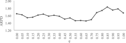
The NEHCG parameter $\eta$ is calibrated on a specially created test platform to separate the calibration benchmark from the test benchmark. The tested benchmark includes 120 instances, wherein $n\in \{20,50,100,200,500\}$ and $m\in \{5,10,20\}$. The value of $\eta$ is selected from the range $[0,1.0]$ with a step size of 0.05. The ARPD values of the NEHCG with different $\eta$ values are shown in Figure 1, and the NEHCG heuristic exhibits the best performance when $\eta =0.65$. Hence, $\eta =0.65$ is recommended in this study. It is worth noting that similar results are obtained for values of $\eta$ in the range $[0.55,0.6]$. This demonstrates the robustness of the parameter selection.

Figure 1 Performance of the NEHCG heuristic with different η values for the calibration benchmark. ARPD = average relative percentage deviation.

Different parameters of the compared algorithms are also calibrated using the test set mentioned in the previous paragraph, and the parameters are given directly. For NNEH, $\alpha =0.1$. For NHPF1 and NHPF2, the values of $\mu$ and $\lambda$ are 0.5 and 0.4, respectively. For tPF_NEH($x$), $\mu =0.35$ is adopted. For a fair comparison, $x$ is set to 1, and δ is 20 for PW_NEH($x$), PFT_NEH($x$) and tPF_NEH($x$). For MBGA, the population size, number of iterations, probability of crossover and probability of mutation are set to 100, 20, 0.8 and 0.9, respectively. Binary tournament selection, two-point crossover and shift mutation operators are used.

In a real manufacturing environment, the value of the weight of the objective, $w$, can be adjusted according to the decision preferences of different BFSPs. Small- and medium-sized manufacturing enterprises based on the ‘make-to-order’ model often have many urgent orders and need to respond quickly, and thus the makespan should be assigned a greater weight. However, high-tech enterprises need to consider machine utilization costs and minimize machine idle time during the processing cycle, thereby reducing the weight of the makespan. To assess the performance of each algorithm under different values of $w$ ($w=\{0,0.1,0.2,\dots ,1\}$), experiments were conducted using the Taillard benchmark. Comparison results are summarized in Tables 4 and 5. The best performance results are highlighted in bold.

Table 4 Average relative percentage deviation (ARPD) of simple constructive heuristics with different w values for the Taillard benchmark (%).

	w
Algorithm	1	0.9	0.8	0.7	0.6	0.5	0.4	0.3	0.2	0.1	0	Average
NEH	1.74	2.43	2.76	2.89	2.87	3.01	2.99	3.05	3.09	3.15	3.16	2.83
NEH_D	1.42	2.22	2.66	2.83	2.69	2.73	2.81	2.87	2.98	2.99	3.07	2.66
NEHKK1	1.76	2.55	2.78	2.82	2.86	2.97	3.02	3.13	3.26	3.28	3.31	2.89
NEHKK2	1.87	2.48	2.81	3.06	3.12	3.15	3.21	3.44	3.49	3.41	3.43	3.04
NEH_WPT	1.59	2.31	2.86	3.08	3.14	3.32	3.43	3.56	3.47	3.56	3.52	3.08
NEHLJP	1.46	2.23	2.58	2.67	2.67	2.84	2.90	3.01	3.11	3.22	3.24	2.72
NNEH	1.68	2.44	2.95	3.06	3.00	3.22	3.30	3.31	3.37	3.44	3.44	3.02
NEHCG	1.41	2.15	2.60	2.65	2.67	2.65	2.88	2.95	2.97	3.01	3.05	2.64

Table 5 Average relative percentage deviation (ARPD) of heuristic algorithms combining the profile-fitting (PF) procedure and Nawaz–Enscore–Ham (NEH) insertion with different w values for the Taillard benchmark (%).

	w
Algorithm	1	0.9	0.8	0.7	0.6	0.5	0.4	0.3	0.2	0.1	0	Average
PFE	1.38	1.90	2.15	2.34	2.33	2.36	2.45	2.50	2.58	2.63	2.65	2.30
NHPF1	1.64	2.29	2.67	3.04	3.12	3.11	3.16	3.34	3.44	3.35	3.37	2.96
NHPF2	1.67	2.36	2.64	2.99	3.03	3.17	3.26	3.33	3.36	3.36	3.37	2.96
PW_NEH	0.84	0.93	1.18	1.21	1.18	1.21	1.28	1.37	1.40	1.43	1.39	1.22
tPF_NEH	0.86	1.05	1.21	1.32	1.35	1.49	1.55	1.53	1.60	1.62	1.60	1.38
PFT_NEH	1.11	1.50	1.65	1.89	1.86	1.91	2.03	2.06	2.16	2.16	2.16	1.86
PW_NEHCG	0.83	0.96	0.92	0.96	0.84	0.85	0.82	0.80	0.84	0.87	0.85	0.87

The results in Table 4 indicate that of the simple constructive heuristics, the NEHCG algorithm achieves the best results for most values of $w$, which demonstrates its effectiveness. Table 5 reveals that the PW_NEHCG algorithm achieves the best results for 10 of 11 values of w among the algorithms combining the PF approach and NEH insertion procedure. As the weights of the IT and BT increase, PW_NEHCG performs better, indicating the superiority of PW_NEHCG for solving the BFSP.

As can be seen from Tables 4 and 5, the performance of the algorithms is different under different $w$ values, indicating that the IT and BT are different from the makespan, although they may be related. PW_NEHCG performs better than NEHCG, which is expected because the initial solution generated in the PW_NEHCG algorithm explores the specific characteristics of the BFSP.

To reconcile the two objectives, it makes sense to define $w$ as 0.5, as the IT, BT and makespan are all measures of time, which is a precious and finite resource for manufacturing (Liu, Jin, and Price 2016). Hence, $w=0.5$ is selected for further testing of the algorithm performance.

5.2. NEHCG algorithm performance

The performance of each simple constructive heuristic is tested for the Taillard, VRF and a randomly generated benchmark, as shown in Table 6. The best performance results are shown in bold. The NEHCG algorithm performs best for the Taillard benchmark, followed by NEH_D, NEHLJP, NEHKK1, NEH, NEHKK2, NNEH and NEH_WPT. Similar results are obtained for the VRF benchmark and the randomly generated benchmark. The detailed computational results of the NEHCG heuristic as well as the performance of the new priority and tie-breaking rules can be seen at https://doi.org/10.6084/m9.figshare.16908529.

Table 6 Average relative percentage deviation (ARPD) of each simple constructive heuristic for the Taillard, Vallada–Ruiz–Framinan (VRF) and randomly generated benchmark (%).

Algorithm	Taillard	VRF	Randomly generated benchmark
NEH	3.01	2.81	3.04
NEH_D	2.73	2.80	2.95
NEHKK1	2.97	2.86	3.00
NEHKK2	3.15	2.92	3.13
NEH_WPT	3.32	3.47	3.37
NEHLJP	2.84	2.75	2.95
NNEH	3.22	3.00	3.21
NEHCG	2.65	2.71	2.84

As can be seen from Table 6, the performance of existing heuristics fluctuates greatly for different test sets, indicating that the two objectives of the makespan and machine utilization sometimes conflict. The results for the three benchmarks indicate that NEH_D and NEHLJP perform better than NEH, NEHKK1, NEHKK2, NNEH and NHE_WPT, which can be attributed to their consideration of the job processing time distribution in the priority rule. Clearly, NEHCG achieves the best results on all three benchmarks, demonstrating its effectiveness.

The Friedman test, followed by the Wilcoxon signed-rank test, is employed to evaluate the statistical difference between heuristics because these tests have been widely used in PFSPs (Fernandez-Viagas, Ruiz, and Framinan 2017). The results are presented in Table 7. The blackened numbers denote a statistically significant difference between the NEHCG algorithm and other simple constructive algorithms. When the confidence level is set to 0.05, the p-value computed using the Friedman test for the Taillard benchmark is zero, indicating that there are significant differences between the compared algorithms. In the post hoc analysis using the Wilcoxon signed-rank test, there are no significant differences between NEHCG, NEH_D and NEHLJP. This is because of the small size of the Taillard test set (Kalczynski and Kamburowski 2008; Fernandez-Viagas and Framinan 2014). The test results for the VRF benchmark show that NEHCG does not differ significantly from NEH, NEH_D and NEHLJP. This occurs because both the Taillard and VRF benchmarks were designed for the makespan rather than the bicriteria problem studied. For the randomly generated benchmark, there are significant differences between NEHCG and the other algorithms.

Table 7 Results of the Friedman test followed by the Wilcoxon signed-rank test for simple constructive heuristics.

		Taillard		VRF		Randomly generated benchmark
Index	Algorithm	Friedman p-value	Wilcoxon p-value	Friedman p-value	Wilcoxon p-value	Friedman p-value	Wilcoxon p-value
1	NEH-NEHCG	0.000	0.001	0.000	0.144	0.000	0.000
2	NEH_D-NEHCG		0.283		0.109		0.031
3	NEHKK1-NEHCG		0.001		0.028		0.000
4	NEHKK2-NEHCG		0		0.000		0.000
5	NEH_WPT-NEHCG		0		0.000		0.000
6	NEHLJP-NEHCG		0.055		0.647		0.029
7	NNEH-NEHCG		0		0.000		0.000

Note: VRF = Vallada–Ruiz–Framinan.

5.3. PW_NEHCG algorithm performance

Table 8 summarizes the performance of the heuristics combining the PF approach and NEH insertion procedure for the Taillard, VRF and the randomly generated benchmark, and the details are presented at https://doi.org/10.6084/m9.figshare.16908529. The numbers in bold in Table 8 represent the results for best performance. PW_NEHCG achieves the best results for the Taillard benchmark, followed by PW_NEH($x$), tPF_NEH($x$), PFT_NEH($x$), PFE, NHPF1 and NHPF2. For the same benchmark, NEHCG is the best of the simple constructive heuristics, but most of the algorithms combining the PF and NEH heuristics perform better than NEHCG, including PFE, PW_NEH, PFT_NEH and TPF_NEH($x$). This shows that the exploration of the specific characteristics of the problem by the PF procedure contributes to better solutions. For 10 of the 12 scales of the test set, PW_NEHCG achieves the best results, which demonstrates its superiority.

Table 8 Average relative percentage deviation (ARPD) of each constructive heuristic combining the profile-fitting (PF) approach and Nawaz–Enscore–Ham (NEH) insertion procedure for Taillard, Vallada–Ruiz–Framinan (VRF) and randomly generated benchmark (%).

Algorithm	Taillard	VRF	Randomly generated benchmark
PFE	2.36	2.88	2.48
NHPF1	3.11	3.47	3.22
NHPF2	3.17	3.48	3.20
PW_NEH(x)	1.21	1.51	1.32
tPF_NEH(x)	1.49	1.78	1.56
PFT_NEH(x)	1.91	2.62	1.88
PW_NEHCG	0.85	0.77	0.95

For the VRF benchmark. PW_NEHCG achieves the best results for 40 of the 48 instances, which further confirms the effectiveness of the PW_NEHCG. For the randomly generated benchmark, it is clear that PW_NEHCG has the best performance, followed by PW_NEH($x$), tPF_NEH($x$), PFT_NEH($x$), PFE, NHPF1 and NHPF2.

It can be seen from Table 8 that PW_NEH($x$), tPF_NEH($x$) and PFT_NEH($x$) heuristics, where the NEH is only applied to the final δ jobs, are superior to PFE, NHPF1 and NHPF2, where the NEH is applied to the whole sequence. The main reason is that the advantage of exploring specific features of the BFSP provided by the PF approach is well exerted when the NEH is only applied to a partial sequence.

The Friedman test followed by the Wilcoxon signed-rank test are used to evaluate the significant differences between PW_NEHCG and the other algorithms combining the PF approach and NEH heuristic. The results are presented in Table 9. When the confidence is set to 0.05, PW_NEHCG is significantly different from the other heuristics for the Taillard, VRF and randomly generated benchmarks.

Table 9 Results of the Friedman test followed by the Wilcoxon signed-rank test for constructive heuristics combining the profile-fitting (PF) approach and Nawaz–Enscore–Ham (NEH) insertion procedure.

		Taillard		VRF		Randomly generated benchmark
Index	Algorithm	Friedman p-value	Wilcoxon p-value	Friedman p-value	Wilcoxon p-value	Friedman p-value	Wilcoxon p-value
1	PFE-PW_NEHCG	0.000	0.000	0.000	0.000	0.000	0.000
2	NHPF1-PW_NEHCG		0.000		0.000		0.000
3	NHPF2-PW_NEHCG		0.000		0.000		0.000
4	PW_NEH(x)-NEHCG		0.005		0.000		0.000
5	tPF_NEH(x)-NEHCG		0.000		0.000		0.000
6	PFT_NEH(x)-NEHCG		0.000		0.000		0.000

Note: VRF = Vallada–Ruiz–Framinan.

5.4. Comparison of heuristics with metaheuristics

To explain the differences in solution quality and running time between heuristic and metaheuristic algorithms in solving the studied multi-objective BFSP, the heuristics are compared with MBGA, which is an improved algorithm based on NSGA-II. MBGA is adapted for the studied problem. The initial feasible solutions are generated randomly. MBGA obtains a Pareto set of solutions for each instance, each of which includes two objectives: machine utilization and the makespan. The linear weighting method is used to transform the two objective values into a single objective value for each solution, and the solution with the best result is selected to compute the RPD. The algorithm is run 20 times. In this study, an approximate method including the average central processing unit time (ACPU) and average relative percentage time (ARPT) indicators (Fernandez-Viagas, Ruiz, and Framinan 2017) is used to evaluate the computational efficiency. The ACPU is the average CPU time of the algorithm for all instances. ARPT represents the number of cases in which the CPU time of the algorithm is greater than the average CPU time of all algorithms in all instances. A smaller ARPT indicates a faster algorithm. The mathematical expressions are as follows: (34) $\begin{array}{rl}ACP{U}_h& =\frac{{\sum }_{\mathrm{\forall }i}CP{U}_{i,h}}{L}\end{array}$(34) (35) $\begin{array}{rl}ARP{T}_h& =\frac{{\sum }_{\mathrm{\forall }i}\frac{CP{U}_{i,h}-AC{T}_i}{AC{T}_i}}{L}+1\end{array}$(35) (36) $\begin{array}{rl}AC{T}_i& =\frac{{\sum }_{\mathrm{\forall }h}CP{U}_{i,h}}{H}\end{array}$(36) where $CP{U}_{i,h}$ is the running time of instance $i$ with heuristic $h$, $AC{T}_i$ represents the average CPU time of all algorithms compared for instance $i$, L denotes the number of instances, and H is the number of heuristics compared. Each algorithm is run 20 times independently. The comparison results are summarized in Table 10. Owing to limited space, this article only visualizes the results for the Taillard benchmark, as shown in Figures 2 and 3.

Figure 2 Average central processing unit time (ACPU) vs average relative percentage deviation (ARPD) of algorithms on a logarithmic scale for the Taillard instances.

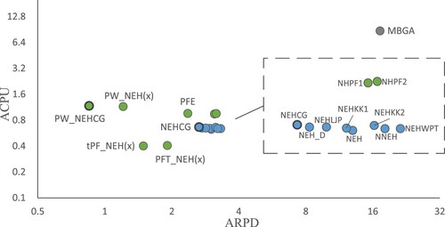
Figure 3 Average relative percentage time (ARPT) vs average relative percentage deviation (ARPD) of algorithms on a logarithmic scale for the Taillard instances.

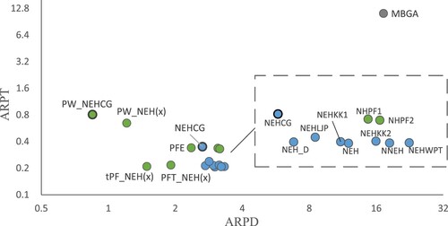
Table 10 Summary of the algorithms in terms of average relative percentage deviation (ARPD), average central processing unit time (ACPU) and average relative percentage time (ARPT).

	Taillard			VRF			Randomly generated benchmark
Algorithm	ARPD	ARPT	ACPU (s)	ARPD	ARPT	ACPU (s)	ARPD	ARPT	ACPU (s)
NEH	3.01	0.206	0.627	2.81	0.360	7.321	3.04	0.230	0.532
NEH_D	2.73	0.213	0.649	2.80	0.363	7.348	2.95	0.234	0.540
NEHKK1	2.97	0.214	0.642	2.86	0.360	7.336	3.00	0.231	0.534
NEHKK2	3.15	0.217	0.660	2.92	0.363	7.346	3.13	0.235	0.540
NEH_WPT	3.32	0.209	0.639	3.47	0.360	7.340	3.37	0.231	0.535
NEHLJP	2.84	0.239	0.649	2.75	0.376	7.357	2.95	0.248	0.540
NNEH	3.22	0.208	0.639	3.00	0.359	7.325	3.21	0.231	0.534
NEHCG	2.65	0.364	0.665	2.71	0.481	7.362	2.84	0.338	0.544
PFE	2.36	0.339	0.957	2.88	0.534	10.390	2.48	0.365	0.815
NHPF1	3.11	0.337	0.943	3.47	0.531	10.303	3.22	0.359	0.804
NHPF2	3.17	0.331	0.952	3.48	0.528	10.352	3.20	0.366	0.818
PW_NEH(x)	1.21	0.645	1.152	1.51	0.754	10.037	1.32	0.662	1.133
tPF_NEH(x)	1.49	0.209	0.401	1.78	0.256	3.699	1.56	0.210	0.373
PFT_NEH(x)	1.91	0.217	0.406	2.62	0.254	3.702	1.88	0.210	0.374
PW_NEHCG	0.85	0.806	1.175	0.77	0.867	10.111	0.95	0.778	1.153
MBGA	17.24	11.245	8.730	14.94	9.250	35.858	16.98	11.070	10.034

Note: VRF = Vallada–Ruiz–Framinan.

Table 10 and Figures 2 and 3 indicate that PW_NEHCG achieves the best ARPD value among all of the reference algorithms, while MBGA does not perform as well as the other algorithms. This is because MBGA cannot search the solution space effectively within a limited computational time. Because NEH is only applied to the last δ jobs, the ACPU values of tPF_NEH($x$) and PFT_NEH($x$) are better than those of PFE, NHPF1 and NHPF2. PW_NEHCG considers the idle time and blocking time generated by the selected job, and the influence of the job on subsequent jobs in generating the initial solution, and adopts the priority rule and tie-breaking rule related to the job processing time distribution. This costs extra computational effort, but also leads to better results. Thus, it can be concluded that PW_NEHCG is the optimal choice for obtaining better solution quality in a reasonable time.

6. Conclusions

This study comprehensively evaluates machine utilization and makespan when solving the BFSP under the RCb* constraint, which has wide applications in industry, especially in cider production. To solve this problem, a simple constructive heuristic, NEHCG, is developed by combining a new priority rule (PRCG) and a new tie-breaking rule (TBCG). Quartile deviation is first applied to the newly proposed priority rule, which can describe the distribution characteristics accurately and obtain a better initial sequence. The new tie-breaking rule is developed by combining the FT and LT rules. To solve the studied BFSP more effectively, an improved constructive heuristic, PW_NEHCG, is presented by effectively combining the NEHCG with an improved PF approach (PW). The new heuristics are tested for three sets of instances (Taillard, VRF and a randomly generated benchmark). Computational experiments show that NEHCG exhibits excellent performance among simple constructive heuristics, and PW_NEHCG further enhances NEHCG by a considerable margin.

In future research, some uncertain factors during production, such as fuzzy processing time (Shao, Pi, and Shao 2020) and machine breakdown situations (Han et al. 2019), should be considered. The development of a robust algorithm for solving the BFSP with uncertain factors is another important research direction.

Disclosure statement

No potential conflict of interest was reported by the authors.

Data availability statement

The data that support the findings of this study are available from the corresponding author upon reasonable request.

References

- Aqil, Said, and Karam Allali. 2021. “On a Bi-criteria Flow Shop Scheduling Problem Under Constraints of Blocking and Sequence Dependent Setup Time.” Annals of Operations Research 296 (1): 615–637. doi: 10.1007/s10479-019-03490-x.
- Deng, G. L., G. D. Tian, X. S. Gu, and S. N. Zhang. 2016. “A Discrete Differential Evolution Algorithm for Multi-objective Scheduling in Blocking Flow Shop.” Huadong Ligong Daxue Xuebao/Journal of East China University of Science and Technology 42 (5): 682–689. doi: 10.14135/j.cnki.1006-3080.2016.05.015.
- Dong, Xingye, Houkuan Huang, and Ping Chen. 2008. “An Improved NEH-Based Heuristic for the Permutation Flowshop Problem.” Computers & Operations Research 35 (12): 3962–3968. https://doi.org/10.1016/j.cor.2007.05.005.
- Fernandez-Viagas, Victor, and Jose M. Framinan. 2014. “On Insertion Tie-Breaking Rules in Heuristics for the Permutation Flowshop Scheduling Problem.” Computers & Operations Research 45: 60–67. https://doi.org/10.1016/j.cor.2013.12.012.
- Fernandez-Viagas, Victor, Rubén Ruiz, and Jose M. Framinan. 2017. “A New Vision of Approximate Methods for the Permutation Flowshop to Minimise Makespan: State-of-the-Art and Computational Evaluation.” European Journal of Operational Research 257 (3): 707–721. https://doi.org/10.1016/j.ejor.2016.09.055.
- Framinan, J. M., R. Leisten, and C. Rajendran. 2003. “Different Initial Sequences for the Heuristic of Nawaz, Enscore and Ham to Minimize Makespan, Idletime or Flowtime in the Static Permutation Flowshop Sequencing Problem.” International Journal of Production Research 41 (1): 121–148. doi:10.1080/00207540210161650.
- Gao, S., Y. Liu, W. Zhang, and J. Zhang. 2007. “Some Supplementation for NEH Heuristic in Solving Flow Shop Problem.” Paper presented at the 2007 American control conference, 9–13 July 2007.
- Han, Y., D. Gong, Y. Jin, and Q. Pan. 2019. “Evolutionary Multiobjective Blocking Lot-Streaming Flow Shop Scheduling With Machine Breakdowns.” IEEE Transactions on Cybernetics 49 (1): 184–197. doi: 10.1109/TCYB.2017.2771213.
- Han, Yuyan, Junqing Li, Hongyan Sang, Yiping Liu, Kaizhou Gao, and Quanke Pan. 2020. “Discrete Evolutionary Multi-objective Optimization for Energy-Efficient Blocking Flow Shop Scheduling with Setup Time.” Applied Soft Computing 93: 106343. https://doi.org/10.1016/j.asoc.2020.106343.
- Kalczynski, P. J., and J. Kamburowski. 2008. “An Improved NEH Heuristic to Minimize Makespan in Permutation Flow Shops.” Computers & Operations Research 35 (9): 3001–3008. doi: 10.1016/j.cor.2007.01.020.
- Kalczynski, P. J., and J. Kamburowski. 2009. “An Empirical Analysis of the Optimality Rate of Flow Shop Heuristics.” European Journal of Operational Research 198 (1): 93–101. doi: 10.1016/j.ejor.2008.08.021.
- Lebbar, Ghita, Abdellah El Barkany, and Abdelouahhab Jabri. 2017. “Multi-criteria Blocking Flowshop Scheduling Problems: Formulation and Performance Analysis.” Paper presented at the 3rd International Conference on Optimization and Applications, Meknes in Morocco, April 28.
- Lebbar, Ghita, Abdellah El Barkany, Abdelouahhab Jabri, and El Abbassi Ikram. 2018. “Hybrid Metaheuristics for Solving the Blocking Flowshop Scheduling Problem.” International Journal of Engineering Research in Africa 36: 124–136. doi: 10.4028/www.scientific.net/JERA.36.124.
- Li, Xiaoping, Qian Wang, and Cheng Wu. 2009. “Efficient Composite Heuristics for Total Flowtime Minimization in Permutation Flow Shops.” Omega 37 (1): 155–164. https://doi.org/10.1016/j.omega.2006.11.003.
- Liang, J. J., Quan-Ke Pan, Chen Tiejun, and Ling Wang. 2011. “Solving the Blocking Flow Shop Scheduling Problem by a Dynamic Multi-swarm Particle Swarm Optimizer.” The International Journal of Advanced Manufacturing Technology 55 (5): 755–762. doi: 10.1007/s00170-010-3111-7.
- Lin, Shih-Wei, Chen-Yang Cheng, Pourya Pourhejazy, and Kuo-Ching Ying. 2021. “Multi-temperature Simulated Annealing for Optimizing Mixed-Blocking Permutation Flowshop Scheduling Problems.” Expert Systems with Applications 165: 113837. https://doi.org/10.1016/j.eswa.2020.113837.
- Liu, W. B., Y. Jin, and M. Price. 2016. “A New Nawaz-Enscore-Ham-Based Heuristic for Permutation Flow-Shop Problems with Bicriteria of Makespan and Machine Idle Time.” Engineering Optimization 48 (10): 1808–1822. doi: 10.1080/0305215x.2016.1141202.
- Maassena, K., P. Perez-Gonzalez, and L. C. Gunther. 2020. “Relationship Between Common Objective Functions, Idle Time and Waiting Time in Permutation Flow Shop Scheduling.” Computers & Operations Research 121: 104965. doi: 10.1016/j.cor.2020.104965.
- McCormick, S. T., M. L. Pinedo, S. Shenker, and B. Wolf. 1989. “Sequencing in an Assembly Line with Blocking to Minimize Cycle Time.” Operations Research 37 (6): 925–935. doi: 10.1287/opre.37.6.925.
- Miyata, Hugo Hissashi, and Marcelo Seido Nagano. 2019. “The Blocking Flow Shop Scheduling Problem: A Comprehensive and Conceptual Review.” Expert Systems with Applications 137: 130–156. https://doi.org/10.1016/j.eswa.2019.06.069.
- Nagano, Marcelo Seido, Adriano Seiko Komesu, and Hugo Hissashi Miyata. 2019. “An Evolutionary Clustering Search for the Total Tardiness Blocking Flow Shop Problem.” Journal of Intelligent Manufacturing 30 (4): 1843–1857. doi: 10.1007/s10845-017-1358-7.
- Nagano, Marcelo Seido, João Vítor Silva Robazzi, and Caio Paziani Tomazella. 2020. “An Improved Lower Bound for the Blocking Permutation Flow Shop with Total Completion Time Criterion.” Computers & Industrial Engineering 146: 106511. https://doi.org/10.1016/j.cie.2020.106511.
- Nawaz, Muhammad, E. Emory Enscore, and Inyong Ham. 1983. “A Heuristic Algorithm for the m-Machine, n-Job Flow-Shop Sequencing Problem.” Omega 11 (1): 91–95. https://doi.org/10.1016/0305-0483(83)90088-9.
- Nouri, Nouha, and Talel Ladhari. 2018. “Evolutionary Multiobjective Optimization for the Multi-machine Flow Shop Scheduling Problem Under Blocking.” Annals of Operations Research 267: 413–430. doi: 10.1007/s10479-017-2465-8.
- Pan, Quan-Ke, and Ling Wang. 2012. “Effective Heuristics for the Blocking Flowshop Scheduling Problem with Makespan Minimization.” Omega 40 (2): 218–229. https://doi.org/10.1016/j.omega.2011.06.002.
- Riahi, Vahid, Mostafa Khorramizadeh, M. A. Hakim Newton, and Abdul Sattar. 2017. “Scatter Search for Mixed Blocking Flowshop Scheduling.” Expert Systems with Applications 79: 20–32. https://doi.org/10.1016/j.eswa.2017.02.027.
- Riahi, V., M. A. H. Newton, K. Su, and A. Sattar. 2019. “Constraint Guided Accelerated Search for Mixed Blocking Permutation Flowshop Scheduling.” Computers & Operations Research 102: 102–120. doi: 10.1016/j.cor.2018.10.003.
- Ribas, Imma, and Ramon Companys. 2015. “Efficient Heuristic Algorithms for the Blocking Flow Shop Scheduling Problem with Total Flow Time Minimization.” Computers & Industrial Engineering 87: 30–39. doi: 10.1016/j.cie.2015.04.013.
- Ribas, Imma, Ramon Companys, and Xavier Tort-Martorell. 2013. “A Competitive Variable Neighbourhood Search Algorithm for the Blocking Flow Shop Problem.” European Journal of Industrial Engineering 7 (6): 729–754. doi: 10.1504/ejie.2013.058392.
- Robazzi, João Vítor Silva, Marcelo Seido Nagano, and Mauricio Iwama Takano. 2021. “A Branch-and-Bound Method to Minimize the Total Flow Time in a Permutation Flow Shop with Blocking and Setup Times.” Paper presented at the 10th international conference of production research. Cham: Springer.
- Ronconi, Débora P. 2004. “A Note on Constructive Heuristics for the Flowshop Problem with Blocking.” International Journal of Production Economics 87 (1): 39–48. https://doi.org/10.1016/S0925-5273(03)00065-3.
- Shao, Zhongshi, Dechang Pi, and Weishi Shao. 2017. “Self-adaptive Discrete Invasive Weed Optimization for the Blocking Flow-Shop Scheduling Problem to Minimize Total Tardiness.” Computers & Industrial Engineering 111: 331–351. https://doi.org/10.1016/j.cie.2017.07.037.
- Shao, Zhongshi, Dechang Pi, and Weishi Shao. 2019. “A Novel Multi-objective Discrete Water Wave Optimization for Solving Multi-Objective Blocking Flow-Shop Scheduling Problem.” Knowledge-Based Systems 165: 110–131. https://doi.org/10.1016/j.knosys.2018.11.021.
- Shao, Zhongshi, Dechang Pi, and Weishi Shao. 2020. “Hybrid Enhanced Discrete Fruit Fly Optimization Algorithm for Scheduling Blocking Flow-Shop in Distributed Environment.” Expert Systems with Applications 145: 113147. https://doi.org/10.1016/j.eswa.2019.113147.
- Spachis, A. S. 1979. “Job-Shop Scheduling with Approximate Methods.” Thesis, Imperial College London (University of London).
- T’kindt, Vincent, and Jean Charles Billaut. 2006. Multicriteria Scheduling: Theory, Models and Algorithms. Berlin: Springer.
- Taillard, E. 1993. “Benchmarks for Basic Scheduling Problems.” European Journal of Operational Research 64 (2): 278–285.
- Tasgetiren, M. F., D. Kizilay, Q. K. Pan, and P. N. Suganthan. 2017. “Iterated Greedy Algorithms for the Blocking Flowshop Scheduling Problem with Makespan Criterion.” Computers and Operations Research 77: 111–126. doi: 10.1016/j.cor.2016.07.002.
- Tasgetiren, M. F., Q. K. Pan, D. Kizilay, and K. Z. Gao. 2016. “A Variable Block Insertion Heuristic for the Blocking Flowshop Scheduling Problem with Total Flowtime Criterion.” Algorithms 9 (4): 71. doi: 10.3390/a9040071.
- Trabelsi, W., C. Sauvey, and N. Sauer. 2012. “Heuristics and Metaheuristics for Mixed Blocking Constraints Flowshop Scheduling Problems.” Computers & Operations Research 39 (11): 2520–2527. doi: 10.1016/j.cor.2011.12.022.
- Vallada, Eva, Rubén Ruiz, and Jose M. Framinan. 2015. “New Hard Benchmark for Flowshop Scheduling Problems Minimising Makespan.” European Journal of Operational Research 240 (3): 666–677. https://doi.org/10.1016/j.ejor.2014.07.033.
- Wang, Ling, Quan-Ke Pan, and M. Fatih Tasgetiren. 2010. “Minimizing the Total Flow Time in a Flow Shop with Blocking by Using Hybrid Harmony Search Algorithms.” Expert Systems with Applications 37 (12): 7929–7936. https://doi.org/10.1016/j.eswa.2010.04.042.
- Wang, Ling, Quan-Ke Pan, P. N. Suganthan, Wen-Hong Wang, and Ya-Min Wang. 2010. “A Novel Hybrid Discrete Differential Evolution Algorithm for Blocking Flow Shop Scheduling Problems.” Computers & Operations Research 37 (3): 509–520. https://doi.org/10.1016/j.cor.2008.12.004.
- Yenisey, M. M., and B. Yagmahan. 2014. “Multi-objective Permutation Flow Shop Scheduling Problem: Literature Review, Classification and Current Trends.” Omega-International Journal of Management Science 45: 119–135. doi: 10.1016/j.omega.2013.07.004.