Understanding the influence of a downstream-side bus stop on saturation flows at an isolated junction

ABSTRACT

This research investigates how saturation flow is affected by bus stops and analyses whether the standard equation used in the UK is adequate for estimating the saturation flow of an approach, especially in the presence of a downstream-side bus stop. As part of the study, we undertook a survey of saturation flows at several junctions in the city of Leeds in England and seek to explain the factors affecting them, taking into account the bus stop located nearby. We develop bootstrapping regression models to explain the difference between the observed and estimated saturation flows and propose an extension to the standard model, accounting for the bus stop located nearby. Finally, this paper illustrates the methods developed and reports on how performance can be improved by reconfiguring a junction.

KEYWORDS:

• Saturation flow
• junction design
• junction performance
• bootstrapping regression
• Practical Reserve Capacity
• case study

1. Introduction

Junctions play a critical role in an urban context affecting the daily commute. According to the UK’s Department for Transport (2020), the average delay on UK’s local ‘A’ roads in 2019 increased by 1.8% from the previous year, which was estimated at 44 s per vehicle per mile. The same report suggests that around major cities, the average delay at junctions was estimated at 20 s per vehicle per mile, which forms a significant proportion of the average delay at more than 45%. Given that the average delay on road networks is steadily increasing, junction delays will also increase as a proportion. Thus, it is critically important to improving junction performance; any weakness in its estimation could lead to inappropriate junction designs, potentially causing significant delays to road users, including public transport. Research on junction performance dates back to the 1960s, when Webster (1963) first introduced the concept of saturation flow. Saturation flow is the maximum number of vehicles that can pass a reference point at a location within a unit duration of time when there is an infinitely long queue. This work was closely followed up with another related study by Webster and Cobbe (1966), in which they performed an extensive study on signalised junctions. These studies clearly indicated that there is a relationship between reserve capacity, degree of saturation, and delay, which make up the main indicators of junction performance.

Since saturation flow is seen as the main building block in measuring the performance of a junction, it is essential to know how to measure this critical variable. Saturation flow can be measured by making observations in the field, or it can be estimated by using the UK Road Research Laboratory’s equation, commonly known as the RR67 equation. Although it is highly recommended that the saturation flow at a location should always be observed, it may not be possible, in practice, due to various constraints. Thus, in the absence of field-based observations, the RR67 equation is routinely used for estimating saturation flow. It is noted that the RR67 equation for unopposed flows depends on lane width, gradient, turning proportion/radius and whether the lane is nearside, or not. Interestingly, it does not account for the presence of bus stops located near junctions that are commonly sighted in urban areas. In the past, there are a number of studies that have focused on delays caused to traffic (both buses and cars) by the presence of bus stops (downstream or upstream), but few have considered how they influence saturation flow and how junction capacity is affected.

We now turn our attention towards public transport to appreciate the views involved in locating a bus stop. Embracing public transport in recent times has helped in reviving the popularity of the public bus, as witnessed by growing trends in bus patronage (MacPherson et al. 2020; Kronberg et al. 2019; Mo, Kwon, and Park 2014; Bristow et al. 2008). Reduction in the generalised cost of travel has been the biggest cause of this shift. However, recurring problems such as delays at signalised junctions, delays due to too many bus stops along a route, longer bus dwell times due to increased passenger numbers and uncertainties in travel time reliability, etc, have led to a drop in the bus patronage again (Chen et al. 2009; Tirachini 2013; Ma et al. 2019). Planners’ attempts to rely on intelligent transportation systems (ITS) in predicting the in-vehicle time in buses and countdown displays at bus stops have helped in regaining lost bus ridership to some extent (Watkins et al. 2011). These measures, however, have proved largely inadequate in addressing the bulk of the delays, which, in fact, occur at signalised junctions affecting the throughput. Therefore, developing a deeper understanding of delays at junctions, especially those caused by bus stops located nearby, is essential.

Bus operators usually push for the stops located close to junctions to make them convenient for passengers. Ceder, Butcher, and Wang (2015) draw on an extensive range of sources to assess the design of bus stop placement on urban routes and mentions that adding several stops onto a bus route can stimulate ridership because of the reduced access time. However, the user in-vehicle time and supplier cost might also increase due to the acceleration/deceleration, dwell times at additional stops involved, potentially affecting the junction performance. Other researchers (cf. Gu et al. (2014); Furth and SanClemente (2006)) considered how the downstream-side (far-sided) or upstream-side (near-sided) stops affect delays to both bus and car traffic. Thus, whilst considerable research has been carried out on the benefits of locating bus stops downstream-side or upstream-side of an isolated signalised junction, no studies have been found that directly link the location of a bus stop to the performance of a signal-controlled junction. This paper contributes to the research by analysing how the downstream-side bus stop affects the saturation flow and investigates how the junction performance is affected. The paper then goes on to develop a method to correct the saturation flow estimates by taking account of the bus stop located nearby. The paper also discusses how junction performance can be improved by relocating a bus stop.

This paper is divided into six sections. Section 2 reviews the literature on saturation flow measurement/estimation, Section 3 sets out the methods for undertaking this research, Section 4 describes the data collection and modelling work undertaken, and Section 5 applies the models to a typical junction and analyses the junction performance by relocating a bus stop. Section 6 concludes the work.

2. Literature review

Research into saturation flow measurement and estimation has a long history, and the earliest investigations were done by Greenshields, Schapiro, and Ericksen (1946); however, it is Webster (1963) who made a significant contribution towards defining a robust measurement technique. Based on the definition stated in the previous section, the literature has presented two measurement methods. Firstly, the ‘classified counts method’ developed by (Webster 1963), where the numbers of vehicles in a queue passing the stop line are recorded at short time intervals during a saturated period. This method is likened to the Canadian Capacity Guide method, which uses the stop line as a reference point, but what differentiates it is the use of the passage of the front bumper as opposed to the rear bumper of the vehicle. Secondly, ‘the headway method’ involves determining the average headways during a specific portion of the green interval where headways are determined when the front bumper crosses the reference point (Branston and van Zuylen 1978; Teply and Jones 1991; Turner and Harahap 1993).

Many researchers have tried to come up with simplified methods to estimate saturation flows, especially where field measurement is impractical. The earliest of these studies was done by Webster and Cobbe (1966), in which they selected 100 signal-controlled junctions to develop relationships between saturation flow rate and the factors affecting it, such as lane width, gradient, turning proportions/radius, etc. Branston and van Zuylen (1978) made further developments to Webster’s estimation technique in which they used multiple linear regression by using synchronous and asynchronous counting methods. Shanteau (1988) proposed the use of the ‘cumulative curve’ of a saturated phase to derive estimates representing the number of vehicles entering an intersection by a specified time after the signal changes to green.

Kimber, Hounsell, and McDonald (1986) came up with a predictive model representing the vehicle exiting progression from a single lane having unopposed traffic, and this equation is still relevant to date. This equation was termed the RR67 equation and is given by: (1) $S=\frac{\left(S_O-140{\delta }_n\right)}{\left(1+1.5f/r\right)}\mathrm{a}\mathrm{n}\mathrm{d}{S}_0=2080-425G{\delta }_g+100\left(W_i-3.25\right)\left[\mathrm{p}\mathrm{c}\mathrm{u}/\mathrm{h}\right]$(1) where S is the saturation flow, ${\delta }_n$ is the nearside lane dummy variable; ${\delta }_g$ is the gradient dummy variable; W_i is the lane width at entry (m); f is the proportion of turning vehicles in a lane; r is the radius of curvature of vehicle paths (m); and G is the gradient (percent).

Equation (1) develops a model to estimate the saturation flow considering the lane width, gradient, whether the lane is nearside and the turning proportion/radius. However, as noted earlier, bus stop locations significantly affect the junction throughput and, thus, the relationship needs to be extended. In this research study, we shall make use of the field measurement techniques that were developed by Webster (1963) and compare the results with the estimated values by using Equation (1) as suggested by Kimber, Hounsell, and McDonald (1986).

Gallivan and Heydecker (1988) and Wood, Crabtree, and Gutteridge (2004) postulated the importance of achieving good control performance at signal-controlled junctions as a pre-requisite for them to perform efficiently, and added that this has helped in reducing emissions, delays and congestion. The term, ‘junction performance’, embodies a multitude of concepts, but Transport for London (2010) describes it as the one which broadly revolves around the ability to establish a relationship between traffic delay and the degree of saturation. Akcelik (1981) proposed performance indicators that could be used to test the efficiency of signal-controlled junctions but mentioned that delay, capacity, degree of saturation and the number of stops are the fundamental performance measures from which other secondary measures (such as vehicle emissions, fuel consumption, vehicle operating costs and value of time) are derived.

A similar study by Hall (1986) using linear regression developed a relationship between accident frequency, traffic flow, pedestrian flow and geometric control features to determine junction performance as an aid to design improvements and remedial measures. The use of qualitative case studies is a well-established approach in assessing the effectiveness of a theorised method in real-life situations. Branston and van Zuylen (1978) and Branston and Gipps (1981) provided early examples of research in multiple linear regression at traffic signals to study factors affecting junction performance. Their studies were aimed at establishing saturation flows, green times and passenger car units using multiple linear regression techniques. The equations derived from both these studies were applied on several sites and proved to be effective and fit for purpose.

Yang et al. (2009), in their study from China, investigated how a bus stop downstream in a mixed traffic, multiple lane situation, affected the car and bicycle streams. Their study showed that the capacity of car traffic was influenced by both bus and cycle streams. In the event that a bus was at a bus stop, traffic streams in the lane would have to look for gaps in an adjacent lane such that they can change lanes while queuing at the back of a halted bus. They concluded that their road capacity model, based on gap acceptance theory and queuing theory for mixed traffic flow at a kerbside bus stop, could be used in traffic analysis and design of bus stops in developing cities.

What we know about bus stop location in relation to junction performance is largely based upon empirical modelling studies that investigate how individual (primary or secondary) junction performance parameters (car delay, bus stop distance, bus delay) are affected by bus stop location, either upstream, or downstream (Wong et al. 1998; Furth and SanClemente 2006; Gu et al. 2014; Lee, Wong, and Li 2015) These researchers have all made a case through modelling and simulations on junction performance parameters suggesting that the location of bus stops has a significant impact on overall performance. However, none have developed models explicitly linking the performance of a junction with the location of a bus stop.

From the review of the available literature, it is evident that among the factors explored in various models, bus stop location at an isolated signalised junction was vital. But, in their recommendations for future research, they suggested that understanding how other related factors work together as in a system to improve (or reduce) junction performance should be explored. This paper precisely addresses this gap identified in the literature and aims to develop a model to estimate the saturation flow at an isolated signal-controlled junction by considering the location of a bus stop.

3. Methods

Regression analysis falls under the category of General Linear Models (GLM), which helps in describing the relationship between predictor (independent) variables and a predicted (dependent) variable (Madsen and Thyregod 2011). The assumptions underlying the use of GLM are that errors are normally distributed while all variables are Multivariate Normal, relationships between the independent and dependent variables are linear, that there is little or no multicollinearity in the data, and the residuals are equal across the regression line (homoscedasticity).

3.1. Multiple linear regression with interaction variables

Salkever (1976) describes that multiple linear regression analysis is often applied to either time-series or cross-section data for the purpose of generating and testing predictions. They add that it entails estimation of coefficients, prediction and prediction of errors, and estimating predicted error variances and confidence intervals.

Harrell Jr (2015) asserts that assuming we denote Y as the response (dependent) variable, X = X₁, X₂, X₃, … . X_n denotes predictor (independent) variables that are presumed to be constant for a specific population, and β = β₀, β₁, β₂, β₃, … , … , β_n denotes the regression coefficients (parameters), but β₀ is an intercept parameter, β₁, …  … , β_n are the corresponding weights of the predictor variables and u is the stochastic error term. Then Y is given by: (2) $Y={\text{β}}_0+{\text{β}}_1{X}_1+{\text{β}}_2{X}_2\dots \dots \dots ..{\text{β}}_n{X}_n+u$(2)

Supposing the predictor variables X₁ and X₂ in the equation above are related whereby the effect of predictor X₁ on response Y depends on X₂ and vice-versa, then an ‘interaction variable’ is introduced that takes the form X₃ = X₁·X₂ (Harrell Jr 2015): (3) $Y={\text{β}}_0+{\text{β}}_1{X}_1+{\text{β}}_2{X}_2+{\text{β}}_3{X}_1{X}_2+u$(3)

Dummy variables in regression analysis take the value of 0 or 1 to indicate the absence or presence of a categorical effect on the value of the predicted variable. Interaction variables introduced above could be dummy variables that account for the joint effect of two (or more) dummy variables.

3.2. Bootstrapping regression

Stine (1989), Davison and Hinkley (1997) and Boos (2003) supported bootstrapping as a nonparametric resampling technique commonly used for estimating standard errors, confidence intervals, sampling variance, significance levels for tests under a null hypothesis and overcoming fewer degrees of freedom problem. They also stress the importance of the bootstrap resampling technique in statistical inference, especially in situations where the population variance is unknown, and the sample size is small. However, they add that where correlated observations are present the bootstrap technique will give incorrect standard error estimations, hence it must be used with caution.

There are two methods of conducting a bootstrap. The first, treats regressors as random, entailing repeated picking from an observed sample, while the second treats regressors as fixed, assuming repeated sampling from fitted residuals of the model. In this study, we directly resample the response variables, treating the regressors as random.

3.3. Junction design

The design of traffic signals and the assessment of junction performance were carried out using LinSig software produced by the JCT Consultancy. The full model building uses the following sequence of steps, summarised from the LinSig User Manual (JCT 2018):

• Building the network

• Traffic flow inputs

• Signal control data input

• Inter-greens, phasing/staging

• Optimisation – cycle time/PRC.

Building the network will need adding junctions (single or multiple numbers of junctions). Then the entry arms need to be defined along with the number of lanes on each arm. The lanes on each entry arm need to be connected to lanes on exit arms. Then the lane details and saturation flow rates need to be added in to configure the junction. Note that the saturation flow rates are calculated using the RR67 equation described earlier unless the modeller wishes to override with specific values to enter. In the next step, traffic zones and flows between them need to be added. Signal control input includes adding phases (traffic and pedestrian) and linking them to lanes already added earlier. Defining the give-way properties of lanes will define the opposed right turns (for UK-style driving). The next step is to add inter-greens as measured. Then add stages and allocate phases to stages. Any prohibited movements such as one-way streets need to be defined too. This will complete the model building, and signal cycle/Practical Reserve Capacity (PRC) optimisation can be undertaken. [See the Appendix for a detailed description of the steps involved in designing a junction.]

4. Numerical studies

4.1. Data collection

In order to address the research question as to whether saturation flow rates are affected by bus stops located downstream, we observed saturation flows based on field measurements which will be compared to estimated flows using the RR67 equation. Additionally, bus stop location distances, bus frequency data and bus lay-by entry/exit angles were also collected. Moreover, we noticed that there are cycle lanes present at some locations; thus cycle lane inventory was also collected. These form part of the data input required for linear regression modelling described later in this section. Sites with saturated traffic conditions during peak hours were selected for observation. Before we start describing the survey locations and the data collected in detail, it is useful to appreciate different types of bus stops that are commonly in use.

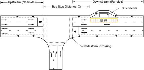
Bus stops can be categorised into three types: kerbside bus stops, bus lay-bys (bus bays) and bus boarders. This study will focus on the kerbside and lay-by type bus stops but excludes bus boarders from the scope. The bus stop distance is defined as the distance from the upstream stop line of an isolated signalised traffic junction to the start of the kerbside bus stop or bus lay-by in the lane at the downstream side of the junction. Figure 1 shows the layout of a typical T-junction and illustrates the terms used, for example, bus stop distance, upstream and downstream sides.

Figure 1. Typical layout of a T-junction.

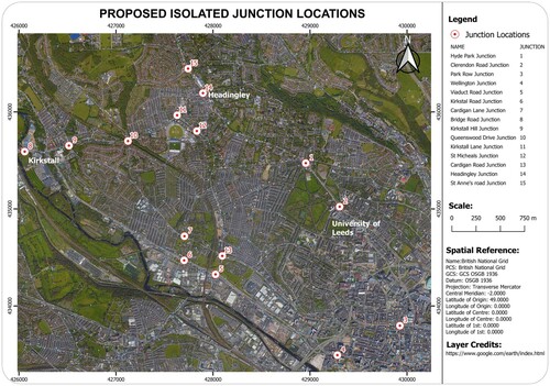
The study was conducted in Leeds, in the areas of Kirkstall, Headingley and Leeds city centre. Fifteen signal-controlled junctions were selected within the three areas for the study, as shown in Figure 2.

Figure 2. Location of junctions in the study area.

4.1.1. Saturation flow count

The saturated period count method is commonly used, which entails measuring saturation flows within a saturated period but allows for the saturation to develop, described as a lag. Lag refers to a suitable interval from the start of green to the first counted vehicle (Teply and Jones 1991; Marler et al. 1993; Turner and Harahap 1993). This lag (or lost time) is usually four vehicles or a 10-second gap, whichever is easier to measure.

The field measurement procedure followed the steps described below:

1. The survey was conducted from 0800 h to 0900 h for the AM peak and 1600 h to 1800 h for the PM peak because they account for the saturated periods;

2. At each of the selected junctions, the traffic flow was observed first to ensure that the conditions were saturated. This was done by ensuring that there wre at least nine vehicles in the queue when the signals were showing ‘RED’;

3. The length of the queue was observed, and the last vehicle to join the queue was identified to make up the full demand at the start of the ‘GREEN’ time;

4. The vehicle progression timing was noted after the fourth vehicle in the queue crossed the stop line allowing for the dissipation of the lost time (lag);

5. The vehicle count commenced only when the fifth vehicle crossed the stop line;

6. The counting of the vehicles and the elapsed time was recorded with the help of a ‘free to download’ software called ‘JCT Traffic Tools’ which is available as an Android-based mobile phone application that aides in saturation flow field data collection;

7. The time elapsed and the number of vehicles discharged during the saturated period was recorded and saved;

8. The recording of the time/vehicles was stopped when the rear of the last vehicle in the saturated queue crossed the stop line; and

9. Steps c to h were repeated for 10 cycles for the unopposed movement.

To compare flows of different vehicle mix, saturation flows are usually expressed in passenger car units (PCUs) in which vehicles are given a value equivalent to the number of cars that they displace from a traffic stream. Transport for London (2010) recommends the PCU values shown in Table 1, which have been used in the study.

Table 1. Passenger car unit conversion factors.

Vehicle type	PCU value
Pedal cycles	0.2
Motorcycles	0.4
Passenger car	1.0
Light goods vehicle (LGV)	1.0
Medium goods vehicle (MGV)	1.5
Buses and coaches	2.0
Heavy goods vehicles (HGV)	2.3
Articulated buses	3.2

Source: Transport for London (2010).

The saturation flow for each cycle was computed using the following equation: (4) $\mathrm{S}\mathrm{a}\mathrm{t}\mathrm{u}\mathrm{r}\mathrm{a}\mathrm{t}\mathrm{i}\mathrm{o}\mathrm{n}\mathrm{f}\mathrm{l}\mathrm{o}\mathrm{w}=\frac{\mathrm{v}\mathrm{e}\mathrm{h}\mathrm{i}\mathrm{c}\mathrm{l}\mathrm{e}\mathrm{s}\left(\mathrm{p}\mathrm{c}\mathrm{u}\right)}{\mathrm{t}\mathrm{i}\mathrm{m}\mathrm{e}\left(\mathrm{s}\mathrm{e}\mathrm{c}\mathrm{o}\mathrm{n}\mathrm{d}\mathrm{s}\right)}\times 3600\left[\mathrm{p}\mathrm{c}\mathrm{u}/\mathrm{h}\right]$(4)

Average observed saturation flow was computed over 10 cycles as the mean of the computed saturation flows obtained by using Equation (4).

4.1.2. Bus stop distance data

Distance to a downstream bus stop was measured from the stop line of the approach lane in metres (see Figure 1) at all the selected isolated junctions using highway and road GIS shapefile data for the Leeds district downloaded from the Consumer Data Research Centre (CDRC) OS Geodata Pack (Singleton and Nguyen 2015). The data collected were then recorded as a predictor variable in a numerical format to be converted later to a dummy variable.

4.1.3. Bus frequency and bus lane data

The bus frequency data for the 15 junctions selected was noted simultaneously while carrying out the saturation flow data collection. The data collected were then validated with the bus operator timetable for the same time period to ensure that variations in recordings, if any, were rationalised. In addition, if there was a bus lane downstream at the junction being surveyed was also noted and transcribed into a dummy variable to be used as a predictor variable in the model.

4.1.4. Cycle lane and pedal cycle frequency data

The cycle lane and pedal cycle frequency data were similarly collected from the site during the field observation survey. Observations were made to note whether there existed a cycle lane downstream, which later was to be transcribed into a dummy variable for analysis in the regression model. Furthermore, whilst counting the throughput progression counts for measuring the saturation flow, pedal cycles were also counted continuously, and the summation was divided by the duration of the survey to obtain pedal cycle frequency for each cycle length.

4.1.5. Traffic data and turning counts

The traffic data and the turning movement data were extracted initially from a SATURN network model of Leeds, which was then updated and validated with the help of limited counts conducted in the year 2019 (see Table A1 in the Appendix).

4.2. Testing the similarity of observed and estimated saturation flow

In this section, we compare the computed, and observed saturation flows using a scatterplot to establish the nature of the relationship between the two sets of data. A preliminary analysis was performed using a scatter plot to compare whether there was a linear association between the two variables (computed and observed saturation flows) – see (Figure 3).

Figure 3. Scatterplot of observed and computed saturation flows.

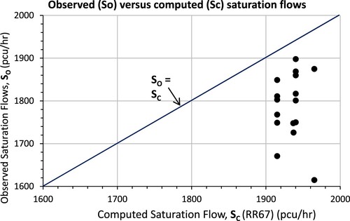
From the scatterplot, the observed saturation flow values are systematically smaller compared to the computed saturation flow values. The highest and least values of the observed saturation flow were 1898 and 1615 pcu/h, respectively, while the computed saturation flow values had the highest and least values of 1965 and 1915 pcu/h, respectively. Figure 3 clearly shows that the computed saturation flows were systematically higher than the observed saturation flows. In the ensuing analysis, we test the significance of the hypothesis that the observed and computed saturations are statistically different to each other.

4.1.1. Two-tailed paired samples t-test

In our study, since we are comparing the results from two different measurement methods for the same set of junction locations, a two-tailed paired samples t-Test was conducted to examine whether the mean difference of computed saturation flows and observed saturation flows were significantly different. Tables 2 and 3 show that the result of the t-test was significantly based on an alpha value of 0.05, t(15) = 7.36, p < .01, indicating that the null hypothesis, that there is no difference between the two sets of means, can be rejected. This finding suggests that the difference between the mean of computed saturation flows and the mean of observed saturation flows is significantly different from zero. Additionally, the mean of computed saturation flows is significantly higher than the mean of observed saturation flows.

Table 2. Paired samples t-test.

	Paired differences			t-stat	t-crit	df	Sig. (2-tailed)	d
	Mean	Std. deviation	Std. error mean
Difference	141.682	76.909	19.227	7.369	2.13	15	0.000^a	1.84

^a Significant at 99% confidence interval; d represents Cohen’s d.

Table 3. Paired samples statistics.

	Mean	N	Std. deviation	Std. error mean
Computed saturation flows (pcu/h)	1929.81	16	18.862	4.715
Observed saturation flows (pcu/h)	1788.13	16	77.169	19.292

4.3. Regression modelling

The development of regression models was based on relating a dependent variable and a number of independent variables, as discussed in Sections 3.1 and 3.2. In our modelling, the dependent variable is defined as the difference between the computed and observed saturation flows. In terms of independent variables, we have chosen 13 variables in total, including 5 numerical variables, 5 dummy variables and 3 interaction variables, as described in Table 4.

Table 4. Regression model variables.

$\mathit{Y}$ = Difference between computed/estimated saturation flow (pcu/h)	${\mathit{X}}_7$ = Dummy for bus stop within 75 m of the stop line.
${\mathit{X}}_1$ = Bus stop distance (metres).	${\mathit{X}}_8$ = Dummy for cycle lane presence
${\mathit{X}}_2$ = Bus frequency (buses/hour).	${\mathit{X}}_9$ = Pedal cycle frequency (cycles/hour)
${\mathit{X}}_3$ = Dummy for bus lay-by presence	${\mathit{X}}_{10}$ = Dummy for multiple lane presence
${\mathit{X}}_4$ = Entry angle (degrees).	${\mathit{X}}_{11}$ = Interaction Variable 1 ($X_3$·$X_{10}$)
${\mathit{X}}_5$ = Exit angle (degrees).	${\mathit{X}}_{12}$ = Interaction Variable 2 ($X_8$·$X_9$)
${\mathit{X}}_6$ = Dummy for bus lane presence.	${\mathit{X}}_{13}$ = Interaction Variable 3 ($X_8$ ·$X_{10}$)

We ran a correlation analysis with the regression variables and noted that the coefficient values were closer to 0 ranging between 1 or −1. This implies that the variables are not related to each other, and hence it is safe to conclude that there is no multicollinearity in the data. In addition to the test of correlation, we have tested the data for linearity (by plotting residuals), Normality of residuals (${\chi }^2$-test of Normality) and heteroscedasticity (Breusch–Pagan test). The results of these tests are not included in the paper for brevity, though available on request.

Since the sample size was small relative to the number of independent variables, the results of the regression model fitting and calibration, however, were not significant (not shown in the paper). The p-values were not significant at the 95% confidence interval. Similarly, the t-statistic values obtained for the models were inside the range of −2 and +2 with large p-values, indicating that the coefficient estimates are insignificant (Gunst and Mason, 1980). In order to have a reasonable sample for the regression analysis, a bootstrapping technique was applied to increase the sample size as described in Section 3.2 and generated a sample of 1000 observations by repeated sampling. The bootstrapping regression model results are shown in Table 5. These models will be used to compute the correction factor to be applied to the computed saturation flow to account for the influence of the bus stop location at isolated junctions.

Table 5. Regression analysis model results.

Variable	Model 1		Model 2
	Coefficient	p-Value	Coefficient	p-Value
Intercept	95.859	.000*	98.000	.000*
X1	–	–	–	–
X2	6.161	.000*	6.571	.000*
X3	−166.623	.000*	−130.481	.000*
X4	−7.354	.000*	−4.629	.000*
X5	16.092	.000*	12.068	.000*
X6	−139.347	.000*	−152.341	.000*
X7	67.474	.000*	53.238	.000*
X8	239.669	.000*	157.779	.000*
X9	−7.435	.000*	−5.631	.000*
X10	−48.955	.000*	−72.346	.000*
X11	–	–	–	–
X12	–	–	–	–
X13	−105.419	.000*	–	–
R^2	0.855		0.801
Adjusted R^2	0.854		0.799
F-test	$F_{10,989}$ = 584.174, p = .000*		$F_{9,990}$ = 443.071, p = .000*
Observations	1000		1000

* Significant at the 99% confidence interval.

** Significant at the 95% confidence interval.

*** Significant at the 90% confidence interval

4.4. Correction factor for RR67 equation

The correction factor for bus stop location C_b is the dependent variable of the linear regression equation, which is equal to the difference between the computed saturation flow (using RR67 equation) and the observed saturation flows (field measured saturation flows): (5) $C_b=S_C-S_O\left[pcu/hr\right]$(5)

The predictive correction factor models for saturation flow were as follows:

Model 1 – (All variables except bus stop distance, Interaction variable 1 and interaction variable 2). (6) $C_b=95.86+6.16B_f-166.62{\delta }_{lb}-7.35{\theta }_1+16.09{\theta }_2-139{\delta }_{bl}+67.47{\delta }_{bs}+239.67{\delta }_{cl}-7.44P{C}_f-48.95{\delta }_{ml}-105.42\left({\delta }_{cl}{\delta }_{ml}\right)\left[\mathrm{p}\mathrm{c}\mathrm{u}/\mathrm{h}\right]$(6)

Model 2 – (All variables except bus stop distance, Interaction variable 1, Interaction variable 2 and interaction variable 3) (7) $C_b=98+6.57B_f-130.48{\delta }_{lb}-4.63{\theta }_1+12.07{\theta }_2-152.34{\delta }_{bl}+53.24{\delta }_{bs}+157.78{\delta }_{cl}-5.63P{C}_f-72.35{\delta }_{ml}\left[\mathrm{p}\mathrm{c}\mathrm{u}/\mathrm{h}\right]$(7) where

$B_f\mathrm{i}\mathrm{s}\mathrm{t}\mathrm{h}\mathrm{e}\mathrm{b}\mathrm{u}\mathrm{s}\mathrm{f}\mathrm{r}\mathrm{e}\mathrm{q}\mathrm{u}\mathrm{e}\mathrm{n}\mathrm{c}\mathrm{y}\left(\mathrm{b}\mathrm{u}\mathrm{s}\mathrm{e}\mathrm{s}/\mathrm{h}\right)$;

${\delta }_{lb}\mathrm{i}\mathrm{s}\mathrm{t}\mathrm{h}\mathrm{e}\mathrm{p}\mathrm{r}\mathrm{e}\mathrm{s}\mathrm{e}\mathrm{n}\mathrm{c}\mathrm{e}\mathrm{o}\mathrm{f}\mathrm{b}\mathrm{u}\mathrm{s}\mathrm{L}\mathrm{a}\mathrm{y}\mathrm{b}\mathrm{y}\mathrm{d}\mathrm{u}\mathrm{m}\mathrm{m}\mathrm{y}\mathrm{v}\mathrm{a}\mathrm{r}\mathrm{i}\mathrm{a}\mathrm{b}\mathrm{l}\mathrm{e}$; ${\theta }_1\mathrm{i}\mathrm{s}\mathrm{t}\mathrm{h}\mathrm{e}\mathrm{e}\mathrm{n}\mathrm{t}\mathrm{r}\mathrm{y}\mathrm{a}\mathrm{n}\mathrm{g}\mathrm{l}\mathrm{e}\left(\mathrm{d}\mathrm{e}\mathrm{g}\mathrm{r}\mathrm{e}\mathrm{e}\mathrm{s}\right)\left(\mathrm{m}\mathrm{e}\mathrm{a}\mathrm{s}\mathrm{u}\mathrm{r}\mathrm{e}\mathrm{d}\mathrm{a}\mathrm{n}\mathrm{t}\mathrm{i}\mathrm{c}\mathrm{l}\mathrm{o}\mathrm{c}\mathrm{k}\mathrm{w}\mathrm{i}\mathrm{s}\mathrm{e}\right)$; ${\theta }_2\mathrm{i}\mathrm{s}\mathrm{t}\mathrm{h}\mathrm{e}\mathrm{e}\mathrm{x}\mathrm{i}\mathrm{t}\mathrm{a}\mathrm{n}\mathrm{g}\mathrm{l}\mathrm{e}\left(\mathrm{d}\mathrm{e}\mathrm{g}\mathrm{r}\mathrm{e}\mathrm{e}\mathrm{s}\right)\left(\mathrm{m}\mathrm{e}\mathrm{a}\mathrm{s}\mathrm{u}\mathrm{r}\mathrm{e}\mathrm{d}\mathrm{c}\mathrm{l}\mathrm{o}\mathrm{c}\mathrm{k}\mathrm{w}\mathrm{i}\mathrm{s}\mathrm{e}\right)$; ${\delta }_{bl}\mathrm{i}\mathrm{s}\mathrm{t}\mathrm{h}\mathrm{e}\mathrm{p}\mathrm{r}\mathrm{e}\mathrm{s}\mathrm{e}\mathrm{n}\mathrm{c}\mathrm{e}\mathrm{o}\mathrm{f}\mathrm{b}\mathrm{u}\mathrm{s}\mathrm{l}\mathrm{a}\mathrm{n}\mathrm{e}\mathrm{d}\mathrm{u}\mathrm{m}\mathrm{m}\mathrm{y}\mathrm{v}\mathrm{a}\mathrm{r}\mathrm{i}\mathrm{a}\mathrm{b}\mathrm{l}\mathrm{e}$; ${\delta }_{bs}\mathrm{i}\mathrm{s}\mathrm{t}\mathrm{h}\mathrm{e}\mathrm{b}\mathrm{u}\mathrm{s}\mathrm{s}\mathrm{t}\mathrm{o}\mathrm{p}\mathrm{d}\mathrm{i}\mathrm{s}\mathrm{t}\mathrm{a}\mathrm{n}\mathrm{c}\mathrm{e}\mathrm{a}\mathrm{t}<75\mathrm{m}\mathrm{e}\mathrm{t}\mathrm{e}\mathrm{r}\mathrm{s}\mathrm{f}\mathrm{r}\mathrm{o}\mathrm{m}\mathrm{s}\mathrm{t}\mathrm{o}\mathrm{p}\mathrm{l}\mathrm{i}\mathrm{n}\mathrm{e}\mathrm{d}\mathrm{u}\mathrm{m}\mathrm{m}\mathrm{y}\mathrm{v}\mathrm{a}\mathrm{r}\mathrm{i}\mathrm{a}\mathrm{b}\mathrm{l}\mathrm{e}$; ${\delta }_{cl}\mathrm{i}\mathrm{s}\mathrm{t}\mathrm{h}\mathrm{e}\mathrm{p}\mathrm{r}\mathrm{e}\mathrm{s}\mathrm{e}\mathrm{n}\mathrm{c}\mathrm{e}\mathrm{o}\mathrm{f}\mathrm{c}\mathrm{y}\mathrm{c}\mathrm{l}\mathrm{e}\mathrm{l}\mathrm{a}\mathrm{n}\mathrm{e}\mathrm{d}\mathrm{u}\mathrm{m}\mathrm{m}\mathrm{y}\mathrm{v}\mathrm{a}\mathrm{r}\mathrm{i}\mathrm{a}\mathrm{b}\mathrm{l}\mathrm{e}$;

$P{C}_f\mathrm{i}\mathrm{s}\mathrm{t}\mathrm{h}\mathrm{e}\mathrm{p}\mathrm{e}\mathrm{d}\mathrm{a}\mathrm{l}\mathrm{c}\mathrm{y}\mathrm{c}\mathrm{l}\mathrm{e}\mathrm{f}\mathrm{r}\mathrm{e}\mathrm{q}\mathrm{u}\mathrm{e}\mathrm{n}\mathrm{c}\mathrm{y}$; and ${\delta }_{ml}\mathrm{i}\mathrm{s}\mathrm{t}\mathrm{h}\mathrm{e}\mathrm{p}\mathrm{r}\mathrm{e}\mathrm{s}\mathrm{e}\mathrm{n}\mathrm{c}\mathrm{e}\mathrm{o}\mathrm{f}\mathrm{m}\mathrm{u}\mathrm{l}\mathrm{t}\mathrm{i}\mathrm{p}\mathrm{l}\mathrm{e}\mathrm{l}\mathrm{a}\mathrm{n}\mathrm{e}\mathrm{s}\mathrm{d}\mathrm{u}\mathrm{m}\mathrm{m}\mathrm{y}\mathrm{v}\mathrm{a}\mathrm{r}\mathrm{i}\mathrm{a}\mathrm{b}\mathrm{l}\mathrm{e}$.

For Model 1, a multiple regression was carried out to explain how the selected variables could significantly predict the difference between the computed and observed saturation flows. The results of the regression indicated that the model explains 85.5% of the variance and that the model was a significant predictor of the saturation flow difference (F(10,989) = 584.174, p < .001, R² = 0.855, $R_{Adjusted}^2$ = 0.854). All predictors were found to have significantly contributed to the model since they were significant at the 99% confidence interval.

Model 2 is very similar to Model 1 but for the interaction variable $X_{13}$. The results of the regression indicated that the model explains 80.1% of the variance and that the model was a significant predictor of the saturation flow difference (F(9,990) = 443.071, p < .01, R² = 0.801, $R_{Adjusted}^2$ = 0.799). All predictors were found to have significantly contributed to the model since they were significant at the 99% confidence interval.

The use of these two models is such that: Model 1 can be used in situations where both a cycle lane and multiple lanes for the same flow direction exist in a road corridor, and that the interaction between the two attributes will influence the saturation flow; and Model 2 can be used in situations where there is no interaction between any of the selected variables for the same flow direction in a road corridor.

Consequently, having identified the robust models and respective computed saturation flows, these outcomes were then used as inputs to LinSig software to perform the junction design analysis on a typical junction such that the scenarios introduced in the next section can be examined.

5. Improving junction performance

LinSig is used primarily to design (un)signalised junctions. In this research, the ability of LinSig to test a scheme using different modelling scenarios has been useful in determining the operational efficiency of a junction.

In order to make conclusive inferences on the modelling outputs from junction designing, it is essential to define the criteria under which an efficient and effective signalised junction can be benchmarked. Three key performance indicators used in this research are: degree of saturation, Practical Reserve Capacity (PRC) and total delay, which are defined as follows:

Degree of saturation: The ratio of demand flow to the maximum flow that can be passed through a junction under stated conditions;

Practical Reserve Capacity (PRC): The reserve capacity of a junction based on a practical operating level of 90% of its capacity; and

Total delay: Summation of delays on all lanes associated with the junction in pcu-hr.

These performance indicators were explored for the defined scenarios modelled but, additionally, other secondary and incidental parameters, for example, Mean Maximum Queues, were also monitored to obtain a wider picture of traffic performance.

The discussion on how the modelled scenarios are performed in terms of each performance indicator is presented in Section 5.2. But it is important that the baseline model is described clearly before making the comparisons.

5.1. Junction design scenarios

As a test of the robustness of the correction factor models developed in Section 4, we need to examine the change in resultant saturation flows as the core to distinguish between the scenarios. Five scenarios plus a base case scenario have been modelled in LinSig (Table 6).

Table 6. The modelled design scenarios.

Modelled scenario	Description
Base case scenario, S0	The isolated signalised junction with the bus stop located at less than 75 m from the upstream stop line, no cycle lane downstream, no bus lane downstream and no bus lay-by downstream.
Scenario S1	The isolated signalised junction with the bus stop located at more than 75m from the upstream stop line, a cycle lane downstream, a bus lane downstream and no bus lay-by downstream.
Scenario S2	The isolated signalised junction with the bus stop located at less than 75 m from the upstream stop line, no cycle lane downstream, a bus lane downstream and no bus lay-by downstream.
Scenario S3	The isolated signalised junction with the bus stop located at less than 75 m from the upstream stop line, the bus frequency upped to 30 buses/h, no cycle lane downstream, no bus lane downstream and no bus lay-by downstream.
Scenario S4	The isolated signalised junction with the bus stop located at less than 75 m from the upstream stop line, a bus lay-by downstream, no cycle lane downstream and no bus lane downstream.
Scenario S5	The isolated signalised junction with the bus stop located at less than 75 m from the upstream stop line, a cycle lane downstream, no bus lane downstream and no bus lay-by downstream.

We have translated the scenario definitions into parameter values as inputs to Model 1 and implemented the new saturation flows computed in the junction models. The base case scenario S0 is a hypothesised case of a simple junction with a bus stop located within 75 m from the stop line. Scenario S1 moves the bus stop away from the junction together with allowing for a lane to be used by cycles and buses. Scenario S2 is aimed at testing the influence of a bus lane, and scenario S3 considers the situation, what-if the frequency of buses increases without a bus lane. S4 tests the conversion of a bus stop to a lay-by, and S5 allows a lane for exclusive use by cycles. Thus, the junction models needed a few changes to reflect each of the scenarios as appropriate. The modifications included changing the lane usage, expanding to accommodate a cycle lane, converting from a bus stop to a bus lay-by, converting a lane to bus-only, and increasing bus frequency. The next section compares the performance of the junction in each scenario against the base case.

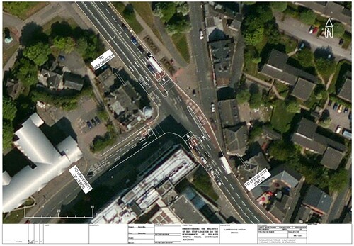
These scenarios were then tested on Clarendon Road junction in Leeds, as shown in Figure 4. It should be noted that from Figure 4, the northbound downstream traffic has multiple lanes, and a shared bus/cycle lane is available; hence, the conditions for the application of Model 1 (rather than Model 2) are satisfied. Another consideration made during the scenario development was that, for every defined scenario, two models consisting of an optimised model and an un-optimised model were tested. This allowed for observations on the change in the PRC and the total delay for the overall model. These performance measures were noted from all models with a cycle time of 120 s which is commonly used in the UK.

Figure 4. Clarendon Road junction.

5.2. Junction performance results

5.2.1. Individual entry lane performance

1. Degree of saturation

The degree of saturation as discussed may be used to inform the junction level of service since it determines vehicular queue and junction delay. Akcelik (1981) mentions that junction performance depreciates when the degree of saturation exceeds 80%. Additionally, Transport for London (2010) points out that beyond 85% degree of saturation, delays start to increase exponentially, and it is on this basis that a 90% degree of saturation was selected as the maximum threshold, beyond which the junction will start operating at negative PRC leading to over-saturated conditions. For the six modelled scenarios, the entry lane degree of saturation was analysed pre- and post-optimisation (unoptimised and optimised situations). The results are shown in Figures 5 and 6 (see the notes below for the entry lane codes used in the figures).

Figure 5. Entry lane degree of saturation for unoptimised modelled scenarios.

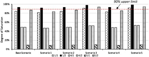
Figure 6. Entry lane degree of saturation for optimised modelled scenarios.

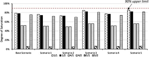
From the results, it is evident that when the six modelled scenarios were optimised for green splits, there was a substantial improvement in the degree of saturation per lane compared to the unoptimised situation. For instance, in the unoptimised situation, Lane 1/2 (A660 Southbound, right-turning traffic) had the highest degree of saturation of 98.5% in the scenario S5. Lane 5/1 (Clarendon Road left turning) had the lowest degree of saturation (10%) among other entry lanes in S5. In the optimised situation, the degree of saturation on Lane 1/2 dropped to 82% in scenario S5. Similarly, the degree of saturation on Lane 5/1 had also dropped to 6.5%, which clearly illustrates the use of optimising.

Examining Figure 6, moving the bus stop away from the junction seems to help in improving the junction performance. Scenario S1 envisages moving the bus stop away from the stop line together with dedicating a lane to cycle/bus use which has resulted in a reduction of about three percentage points in the degree of saturation, which reduces the delays and improves the junction performance. Scenario S2 appears to be the best of all, with the three busiest lanes 1/1, 1/2 and 5/2 operating at a degree of saturation of 70–73%, which is significantly smaller compared to 75–80% in the base scenario S0. In contrast, in scenario S3, which envisages an increase in bus frequency, the degree of saturation on the three busiest lanes increases to 81–85%, clearly indicating the onset of congestion with a higher number of buses passing through the junction. Thus, the strategy of dedicating a lane for the exclusive use of buses, where multiple lanes are present, helps improve junction performance. Finally, converting a bus stop to a bus lay-by improves the junction performance with a 1% reduction in the degree of saturation (scenario S4). Dedicating a lane for cycles alone, however, will lead to a drop in junction performance as the available capacity for motorised vehicles is reduced (scenario S5).

(b)	Mean Maximum Queues

Transport for London (2010) describes the Mean Maximum Queues (MMQ) as the average number of vehicles (pcu) that have been added to the queue until the time when the queue finally dissipates at the stop line. They added that MMQ is synonymous with the position reached by the back of the queue as the queue is discharging during the green period.

In modelling traffic, vehicles are assumed to travel at cruise speed across the link prior to adding to the queue. This is rather like vehicles are piling up vertically at the stop line; however, this is not the case in real-life situations where the queue increases backwards until blocking is caused at the upstream junction. For this reason, there is no specific baseline value or maximum threshold for MMQ, but rather the aim is to reduce it as much as possible. For the six modelled scenarios, the MMQ was analysed prior to optimisation (unoptimised situation), and the post optimisation (optimised situation), and the results are shown in Figures 7 and 8.

Figure 7. Entry lane mean maximum queue for unoptimised modelled scenarios.

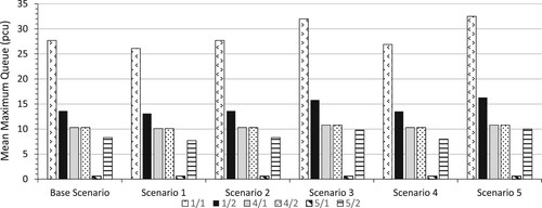
Figure 8. Entry lane mean maximum queue for optimised modelled scenarios.

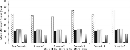
From Figures 7 and 8, it is observed that redesigning and optimising the green splits and offsets of the models with different scenarios improves the junction performance by reducing the MMQ. In both graphs, it is seen that the Lanes 1/1 and 5/1 had the highest and lowest MMQ, respectively. For the unoptimised situation, Lane 1/1 (A660 Southbound, straight ahead) had the highest MMQ with a value of 32.5 pcu experienced in scenario S5. Lane 5/1 (Clarendon Road left turning) had the lowest value (0.6 pcu) in all modelled scenarios. For the optimised situation, on average, Lane 1/1 (A660 southbound, straight ahead) had the largest MMQ value (27.4 pcu) experienced with scenario 5. Like the unoptimised situation, Lane 5/1 had the lowest value (0.5 pcu) amongst all other modelled scenarios. The above observations confirm once again that optimising the signals will hugely help improve junction performance.

As to the question of which strategies might be effective in reducing queue lengths, the commentary made in Figure 6 earlier will be equally applicable to Figure 8. Firstly, moving the bus stop away from the stop line will help reduce the queue lengths (scenario S1). Secondly, creating a bus lane will ease the queuing, as the following vehicles do not have to wait behind a bus at the stop before being able to change lanes (scenario S2). Increased bus frequencies will lead to additional queuing (scenario S3). Converting a bus stop to a bus lay-by marginally helps in reducing the queue lengths. Finally, allowing a lane for bus and cycle use will improve the lane usage, rather than allowing exclusive use by cycles alone (as in scenario S5).

5.2.2. Network summary

The overall network summary results were presented based on PRC and the total delay experienced by all movements at the junction. A summary is provided in Table 7.

Table 7. Network modelling summary results.

Scenario	Unoptimised		Optimised
	PRC (%)	Delay (pcu/h)	PRC (%)	Delay (pcu/h)
Base case scenario (So)	−3.6	25.71	13.5	20.20
Scenario 1	−2.0	23.81	18.0	19.04
Scenario 2	−0.7	22.45	22.3	18.31
Scenario 3	−8.6	32.11	5.6	22.67
Scenario 4	−3.3	24.89	15.7	19.47
Scenario 5	−9.4	33.05	4.9	22.93

From the results in Table 7, we can observe that models performed consistently better after optimisation in terms of both the PRC and total delay. In general, after optimisation, the PRC increased by nearly 18% on average, while the total delay decreased by an average of 6.57 pcu-hr. Scenario S1, which envisages moving the bus stop away from the junction together with a dedicated lane for bus/cycle usage, gains in terms of PRC by reaching 18% compared to 13.5% in the base scenario S0. Scenario S2 performs the best with junction improvement after optimisation with 22.3% and 18.31 pcu-hr for PRC and total delay, respectively – clearly indicating the benefit of providing a dedicated bus lane even with the bus stop located within 75 m from the stop line. The PRC in scenario S3 is low because of the increased bus frequencies; however, this is still a useful design due to the optimisation gains. Scenario S4 indicates that the PRC will improve by converting a bus stop to a bus lay-by. Finally, the scenario S5 model was the least-performing of all with a PRC of 4.9% and 22.93 pcu-hr total delays.

6. Concluding remarks

This research has sought to understand the influence of bus stop location on the performance of signal-controlled junctions in order to assess the saturation flow influenced by the bus stop located on the exit lane, to assess the performance of a junction given the location of the bus stop, and to design the junction by relocating the bus stop to improve the performance.

Regression modelling was performed on data collected from 15 junctions with the help of 13 predictor variables. This dataset was tested for robustness and consistency by carrying out hypothesis testing to check whether there existed a non-zero difference between the computed and observed saturation flows. The results showed that there was a significant difference between the site observed (measured) and the computed (estimated) saturation flows using the RR67 equation. A number of models were then developed but, after testing their robustness in giving realistic and accurate saturation flows, two models were found to be consistent.

With these equations, it was possible to obtain the adjusted saturation flow that accounts for the bus stop located downstream of a junction. Junction design modelling was performed to determine the junction performance on five developed scenarios using the adjusted saturation flow derived by applying the corrective equations developed. Alternative design scenarios were applied to a junction in the city of Leeds, as an illustration of the use of the corrective equations developed.

The results showed that in all instances (scenarios), having multiple lanes increased the saturation flow, but, most importantly, Practical Reserve Capacity (PRC), which is a measure of overall junction performance, increased when the exit had multiple lane configurations. It was also observed that having multiple lanes, of which one of the lanes is a bus lane, also increased the overall junction PRC. Similarly, having a shared bus and cycle lane improved the lane degree of saturation and, therefore, overall junction performance. When the choice of having a bus lay-by over a kerbside bus stop was made, the results showed that having a bus lay-by would be better in terms of overall junction performance. The results also showed that an increase in bus frequency without a bus lane made the junction perform poorly. It was also noted that having a cycle lane reduced the rate at which vehicles egressed past the junction in all instances; however, when a bus lane was shared with pedal cycles and multiple lanes introduced, junction performance greatly improved.

Acknowledgement

The authors would like to thank the Commonwealth Scholarship Commission for funding the second author’s study programme at the University of Leeds, UK. The authors jointly thank JCT Ltd for allowing the use of LinSig software for this research.

Disclosure statement

No potential conflict of interest was reported by the author(s).

Appendix

Junction design procedure.

Step 1 – The Network: The model building follows a meticulous process that includes adding junction components (arms, lanes, connectors), cruise speeds/times, saturation flows, adding zones, adding signal phases and signal controllers. The built network for Clarendon Road junction is presented in Figure A1.

Step 2 – Traffic Flows: The traffic demand flows that were adopted for the study are shown in Table A1.

Step 3 – Lane-based Flow and Bus Modelling: LinSig uses lane-based and layered flows to identify different types of traffic such as buses, cars, etc while also permitting interaction between traffic for each layer (Figure A2). The bus cruise speed adopted was 25 km/h, while the mean bus stopped time was 15 s (JCT 2018).

Step 4 – Inter-green Calculations: The phase inter-green calculations were done using QuickGreen software produced by JCT. The software application aids in the quick calculation of the inter greens through analysis of the conflict distance measurement and eliminating possible geometrical errors that would arise out of hand computations. Lanes, turning paths, signal phases for both vehicular traffic and pedestrians as shown in Figure A3.

The phase inter-green matrix was then generated for the potential conflicting movements as the difference between the clearance distance for the phase gaining and the phase losing the right of way for traffic after a vehicle crosses the stop line (Table A2).

Step 5 – Stage Sequence Setup: The phases for all movements were arranged and set to run together in a sequence avoiding any possible traffic conflict as shown in Figure A4.

The first stage is for northbound, southbound and westbound traffic while restricting all pedestrian movements on the three arms. However, since the north to westbound right-turning movement is conflicting with the northbound straight-ahead traffic, the former gives way to the head traffic. The right-turning lane was designed to hold up to three vehicles as the drivers wait for a gap. Stage 2 allows for only southbound traffic and north to westbound traffic, the pedestrian movements are all restricted. Stage 3 allows for the west to northbound and southbound traffic while restricting all pedestrian movements. Stage 4 is a pedestrian stage that allows for all pedestrian phase movements while restricting all vehicular movements.

Step 6 – Signal Timings: The signal timings view aids the adjustment of the phase and stage timings such that an optimal solution can be reached as shown in Figure A5.

Step 7 – Cycle Time Optimisation: The cycle time must be as low as possible with the aim of minimising pedestrian waiting time, while also getting the best out of the Practical Reserve Capacity (PRC). In this research, since pedestrian modelling was not carried out, the primary aim of optimisation is to maximise the PRC. In LinSig, the cycle time optimisation was undertaken as shown in Figure A6 and a cycle time of 120s was found optimal for the design.

Figure A1. The network layout diagram for the base case scenario.

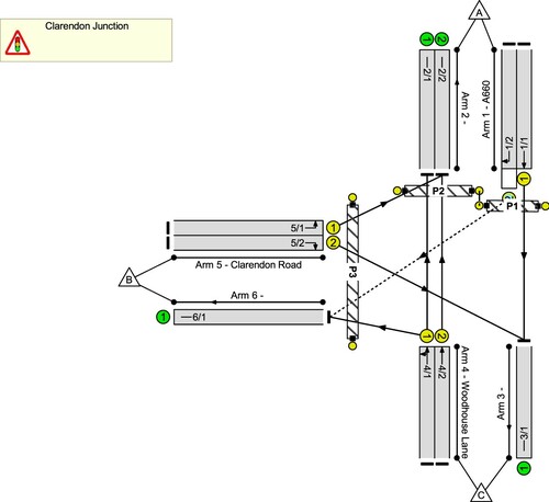
Figure A2. Route flows and lane-based flows for the base scenario model.

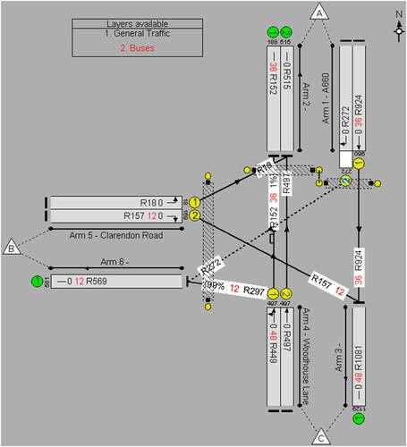
Figure A3. Lanes, turn paths, signal phases and pedestrian crossings.

Figure A4. Signal Stage sequence arrangement for all scenarios

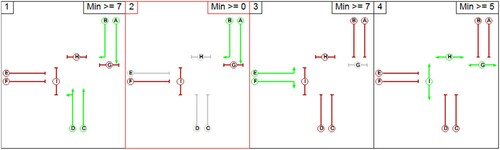
Figure A5. Signal timing for base case scenario.

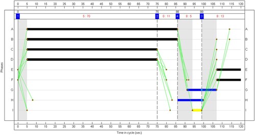
Figure A6. Cycle time optimisation for the junction

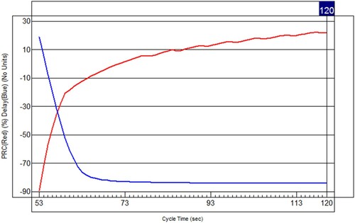
Table A1. Demand flow in pcus/h (2019).

	DESTINATION
		A	B	C	Total
Origin	A	–	352	1243	1595
	B	23	–	219	242
	C	887	400	–	1287
	Total	910	752	1462

Table A2. Phase inter-green matrix (s).

	Starting phase
		A	B	C	D	E	F	G	H	I
Terminating Phase	A	–	–	–	5	–		5	–	–
	B	–	–	5	6	–	6	5	–	8
	C	–	5	–	–	5	5	–	8	–
	D	–	5	–	–	5	5	–	8	7
	E	–	–	5	5	–	–	–	8	5
	F	5	5	5	5	–	–	–	–	5
	G	7	7	–		–	–	–	–	–
	H	–	–	7	7	7	–	–	–	–
	I	–	8	–	8	8	8	–	–	–

References

- Akcelik, R. 1981. Traffic Signals: Capacity and Timing Analysis. Research Report, ARR (123). Port Melbourne: Australian Road Research Board.
- Boos, D. D. 2003. “Introduction to the Bootstrap World.” Statistical Science 18 (2): 168–174.
- Branston, D., and P. Gipps. 1981. “Some Experience with a Multiple Linear Regression Method of Estimating Parameters of the Traffic Signal Departure Process.” Transportation Research Part A: General 15 (6): 445–458.
- Branston, D., and H. van Zuylen. 1978. “The Estimation of Saturation Flow, Effective Green Time and Passenger car Equivalents at Traffic Signals by Multiple Linear Regression.” Transportation Research Part A: General 12 (1): 47–53.
- Bristow, A. L., M. P. Enoch, L. Zhang, C. Greensmith, N. James, and S. Potter. 2008. “Kickstarting Growth in Bus Patronage: Targeting Support at the Margins.” Journal of Transport Geography 16 (6): 408–418.
- Ceder, A., M. Butcher, and L. Wang. 2015. “Optimization of Bus Stop Placement for Routes on Uneven Topography.” Transportation Research Part B: Methodological 74: 40–61.
- Chen, X., L. Yu, Y. Zhang, and J. Guo. 2009. “Analyzing Urban Bus Service Reliability at the Stop, Route, and Network Levels.” Transportation Research Part A: Policy and Practice 43 (8): 722–734.
- Davison, A. C., and D. V. Hinkley. 1997. Bootstrap Methods and Their Application. Cambridge, MA: Cambridge University Press.
- Department for Transport. 2020. Travel Time Measures for the Strategic Road Network and Local ‘A’ Roads: January to December 2019. London: Department for Transport.
- Furth, P. G., and J. L. SanClemente. 2006. “Near Side, Far Side, Uphill, Downhill: Impact of Bus Stop Location on Bus Delay.” Transportation Research Record: Journal of the Transportation Research Board 1971 (1): 66–73.
- Gallivan, S., and B. Heydecker. 1988. “Optimising the Control Performance of Traffic Signals at a Single Junction.” Transportation Research Part B: Methodological 22 (5): 357–370.
- Greenshields, B. D., D. Schapiro, and E. L. Ericksen. 1946. Traffic Performance at Urban Street Intersections. Connecticut, CT: Bureau of Highway Traffic.
- Gu, W., V. V. Gayah, M. J. Cassidy, and N. Saade. 2014. “On the Impacts of Bus Stops Near Signalized Intersections: Models of Car and Bus Delays.” Transportation Research Part B: Methodological 68: 123–140.
- Gunst, R F, and R L Mason. 1980. Regression analysis and its application: a data oriented approach. Marcel Dekker
- Hall, R. D. 1986. Accidents at Four-arm Single Carriageway Urban Traffic Signals. Wokingham: Transport Research Laboratory.
- Harrell Jr, F. E. 2015. Regression Modeling Strategies: With Applications to Linear Models, Logistic and Ordinal Regression, and Survival Analysis. Berlin: Springer.
- JCT. 2018. Linsig 3.2 User Guide. Lincoln: JCT Consultancy Ltd.
- Kimber, R., N. Hounsell, and M. McDonald. 1986. The Prediction of Saturation Flows for Single Road Junctions Controlled by Traffic Signals. Wokingham: Transport Research Laboratory.
- Kronberg, N., S. Weekes, C. Cameron, and P. Sevenel. 2019. Transport Statistics Great Britain 2019. London: Department for Transport.
- Lee, S., S. C. Wong, and Y. C. Li. 2015. “Real-time Estimation of Lane-based Queue Lengths at Isolated Signalized Junctions.” Transportation Research Part C: Emerging Technologies 56: 1–17.
- Ma, J., J. Chan, G. Ristanoski, S. Rajasegarar, and C. Leckie. 2019. “Bus Travel Time Prediction with Real-time Traffic Information.” Transportation Research Part C: Emerging Technologies 105: 536–549.
- MacPherson, H., M. Dickens, D. C. Grisby, W. W. McCarragher, and P. P. Skoutelas. 2020. 2020 Public Transportation Fact Book. 71st ed. Washington, DC: American Public Transportation Association.
- Madsen, H., and P. Thyregod. 2011. Introduction to General and Generalized Linear Models. Boca Raton, FL: Chapman & Hall/CRC.
- Marler, N. W., F. O. Montgomery, P. Disney, G. Gardner, J. C. Rutter, and P. R. Fouracre. 1993. Overseas Road Note 11: Urban Road Traffic Surveys. Wokingham: Transport Research Laboratory.
- Mo, C., Y.-I. Kwon, and S. Park. 2014. Current Status of Public Transportation in ASEAN Megacities. Goyang-daero: Korea Transport Institute.
- Salkever, D. S. 1976. “The Use of Dummy Variables to Compute Predictions, Prediction Errors, and Confidence Intervals.” Journal of Econometrics 4 (4): 393–397.
- Shanteau, R. M. 1988. Using Cumulative Curves to Measure Saturation Flow and Lost Time. Washington DC: Institute of Transportation Engineers.
- Singleton, A., and H. Nguyen. 2015. “CDRC 2015 OS Geodata Pack–Leeds (E08000035).” Accessed May 28, 2019. Available from: https://data.cdrc.ac.uk/dataset/cdrc-2015-os-geodata-pack-leeds-e08000035.
- Stine, R. 1989. “An Introduction to Bootstrap Methods: Examples and Ideas.” Sociological Methods & Research 18 (2-3): 243–291.
- Teply, S., and A. M. Jones. 1991. “Saturation Flow: Do We Speak the Same Language?” Transportation Research Record 1320: 144–153.
- Tirachini, A. 2013. “Estimation of Travel Time and the Benefits of Upgrading the Fare Payment Technology in Urban Bus Services.” Transportation Research Part C: Emerging Technologies 30: 239–256.
- Transport for London. 2010. Traffic Modelling Guidelines: TfL Traffic Manager and Network Performance Best Practice Version 3.0. London: Transport for London.
- Turner, J., and G. Harahap. 1993. Simplified Saturation Flow Data Collection Methods. In: CODATU VI Conference on the Development and Planning of Urban Transport, Tunis, February.
- Watkins, K. E., B. Ferris, A. Borning, G. S. Rutherford, and D. Layton. 2011. “Where Is My Bus? Impact of Mobile Real-time Information on the Perceived and Actual Wait Time of Transit Riders.” Transportation Research Part A: Policy and Practice 45 (8): 839–848.
- Webster, F. V. 1963. A Method of Measuring Saturation Flow at Traffic Signals. Road Note 34. Crowthorne: Road Research Laboratory.
- Webster, F. V., and B. M. Cobbe. 1966. Traffic Signals, Road Research Technical Paper No.56. London: HMSO.
- Wong, S. C., H. Yang, W. S. A. Yeung, S. L. Cheuk, and M. K. Lo. 1998. “Delay at Signal-controlled Intersection with Bus Stop Upstream.” Journal of Transportation Engineering 124 (3): 229–234.
- Wood, K., M. Crabtree, and S. Gutteridge. 2004. Users’ Guide for a Simple Performance Indicator for Traffic Signals. Wokingham: Transport Research Laboratory.
- Yang, X., Z. Gao, X. Zhao, and B. Si. 2009. “Road Capacity at Bus Stops with Mixed Traffic Flow in China.” Transportation Research Record: Journal of the Transportation Research Board 2111 (1): 18–23.