Distinct eigenvalues are realizable with generic eigenvectors

Abstract

Motivated by applications in matrix constructions used in the inverse eigenvalue problem for graphs, we study a concept of genericity for eigenvectors associated with a given spectrum and a connected graph. This concept generalizes the established notion of a nowhere-zero eigenbasis. Given any simple graph G on n vertices and any spectrum with no multiple eigenvalues, we show that the family of eigenbases for symmetric matrices with this graph and spectrum is generic, strengthening a result of Monfared and Shader. We illustrate applications of this result by constructing new achievable ordered multiplicity lists for partial joins of graphs and providing several families of joins of graphs that are realizable by a matrix with only two distinct eigenvalues.

Keywords:

• Symmetric matrix
• join of graphs
• inverse eigenvalue problem
• minimal number of distinct eigenvalues

AMS CLASSIFICATIONS:

• 15B57
• 15A18
• 15B10
• 05C50

1. Introduction

Let G be a simple graph with vertex set $V(G)=\{1,\dots ,n\}$ and edge set $E(G)$, and consider $S(G)$, the set of all real symmetric $n\times n$ matrices $A=\left(\begin{array}{c}a(i,j)\end{array}\right)$ such that, for $i\ne j$, $a(i,j)\ne 0$ if and only if $\{i,j\}\in E(G)$, with no restriction on the diagonal entries of A. The inverse eigenvalue problem for graphs (IEP-G) seeks to characterize all possible spectra $\sigma (A)=\{{\lambda }_1,\dots ,{\lambda }_n\}$ of matrices $A\in S(G)$. The IEP-G is solved for a few families of graphs (complete graphs, paths, generalized stars [1], cycles [2,3], generalized barbell graphs [4], linear trees [5]) and for graphs of order at most 5[6]; the problem remains open in many other cases.

The closely related ordered multiplicity inverse eigenvalue problem for graphs seeks to characterize all possible ordered multiplicities of eigenvalues of matrices in $S(G)$, i.e. to characterize the ordered lists of nonnegative integers $(m_1,\dots ,m_r)$ for which there exists a matrix $A\in S(G)$ and ${\lambda }_1<\cdots <{\lambda }_r$, such that $\sigma (A)=\{{\lambda }_1^{(m_1)},\dots ,{\lambda }_r^{(m_r)}\}$, where ${\lambda }_i^{(m_i)}$ denotes $m_i$ copies of ${\lambda }_i$. We call such an ordered list $(m_1,\dots ,m_r)$ an ordered multiplicity vector of G. The ordered multiplicity inverse eigenvalue problem has been resolved for all connected graphs of order at most 6[7]. For some specific families of connected graphs, several ordered multiplicity vectors have been determined (see, e.g. [4,6,8]). Moreover, Monfared and Shader proved the following theorem in [9], showing that $(1,1,\dots ,1)$ is an ordered multiplicity vector of any connected graph G, which can be realized with a nowhere-zero eigenbasis, that is, a basis of eigenvectors, each containing no zero entry.

Theorem 1.1

[9,Theorem 4.3]

For any connected graph G on n vertices and distinct real numbers ${\lambda }_1,\dots ,{\lambda }_n$, there exists $A\in S(G)$ with spectrum $\sigma (A)=\{{\lambda }_1,\dots ,{\lambda }_n\}$ and an eigenbasis consisting of nowhere-zero vectors.

Our main result, Theorem 2.4, is a strengthening of Monfared and Shader's theorem. We show that we can make considerably more stringent genericity requirements of the eigenbasis than simply asking that it is nowhere-zero; in the language of [10], we show that any spectrum with only simple eigenvalues is generically realizable, for any connected graph G.

Recall that a matrix is nowhere-zero if each of its entries is nonzero. Let $\sigma =\{{\lambda }_1,\dots ,{\lambda }_n\}$ be a multiset of real numbers. For a connected graph G, we say the multiset σ is realizable for G if $\sigma =\sigma (A)$ for some $A\in S(G)$; we say σ is generically realizable for G if, moreover, for any finite set $\mathcal{Y}\subseteq {\mathbb{R}}^n\setminus \{\mathbf{0}\}$ there is an orthogonal matrix U so that $\mathrm{UD}{U}^{\mathrm{\top }}\in S(G)$, where D is a diagonal matrix with spectrum σ and $U\mathbf{y}$ is nowhere-zero for all $\mathbf{y}\in \mathcal{Y}$. (As noted above, this condition is stronger than the realizability of σ in $S(G)$ with a nowhere-zero eigenbasis: consider $\mathcal{Y}=\{{\mathbf{e}}_1,\dots ,{\mathbf{e}}_n\}$.) Let $\mathbb{N}$ be the set of strictly positive integers. An ordered multiplicity vector $\mathbf{m}=(m_1,\dots ,m_r)\in {\mathbb{N}}^r$ is spectrally arbitrary for G if for any real numbers ${\lambda }_1<\cdots <{\lambda }_r$, the multiset $\sigma =\{{\lambda }_1^{(m_1)},\dots ,{\lambda }_r^{(m_r)}\}$ is realizable for G. Further, we say $\mathbf{m}$ is generically realizable for G if it is spectrally arbitrary for G, and every assignment of eigenvalues results in a generically realizable multiset for G, as defined above.

We will also need to deal with disconnected graphs. The notion of the multiplicity matrix of a disconnected graph was introduced in [10] as a generalization of the ordered multiplicity vector of a connected graph, as follows. Let G be a graph with $k\in \mathbb{N}$ connected components $G_1,\dots ,G_k$. For $r\in \mathbb{N}$, an $r\times k$ matrix V with non-negative integer entries is said to be a multiplicity matrix for G if, for $1\le i\le k$, the ith column of V is an ordered multiplicity list realized by a matrix in $S(G_i)$. Note that a trivial necessary condition for V to be a multiplicity matrix of G is that the orders of the connected components of G are the same as the column sums of V; we abbreviate this by saying that V fits G. If every column of a multiplicity matrix V for a graph G is generically realizable for the corresponding connected component of G, then we say V is generically realizable for G.

The methods used in [6,11] to resolve the IEP-G and the ordered multiplicity IEP-G for small graphs make essential use of strong properties. In particular, a symmetric $n\times n$ matrix A is said to have the strong spectral property (the SSP) if the zero matrix 0 is the only symmetric matrix X satisfying AX = XA and $A\circ X=I_n\circ X=0$, where ○ denotes the Hadamard product. The SSP was first defined in [11]. One of its key features is the following perturbation result.

Theorem 1.2

[11,Theorem 10]

Let $G^{\mathrm{\prime }}$ be a spanning subgraph of a graph G. If $A^{\mathrm{\prime }}\in S(G^{\mathrm{\prime }})$ is a matrix with the SSP, then for any $ϵ>0$ there is a matrix $A\in S(G)$ with the SSP such that A and $A^{\mathrm{\prime }}$ have the same eigenvalues and $\Vert A-A^{\mathrm{\prime }}\Vert <ϵ$.

To establish Theorem 2.4, we first prove it for trees, and then apply the SSP in the case that $G^{\mathrm{\prime }}$ is a spanning tree of G. A 0–1 matrix contains only 0s and 1s; casting Theorem 2.4 in this language, we obtain Theorem 2.5: every 0–1 multiplicity matrix which fits a graph G is generically realizable for G. In particular, this implies that every multiplicity matrix which fits a path $P_n$ is generically realizable for $P_n$. In the terminology of [10], we say the graph $P_n$ is generically realizable.

Figure 1. Sketch of the partial join $(P_7,X)\vee H$, where pendant vertices X of $P_7$ are coloured grey. The edges of H are not drawn.

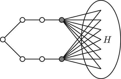
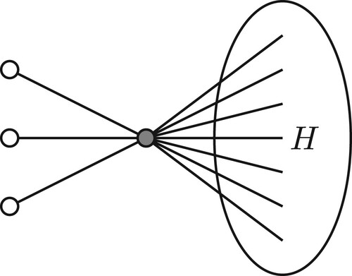
Figure 2. Sketch of the partial join $K_1\vee (3K_1\cup H)$, where the high degree vertex v is coloured grey. The edges of H are not drawn.

We provide some applications in Section 3. In particular, we are interested in finding examples of joins of graphs that allow a small number of distinct eigenvalues. The minimum number of distinct eigenvalues of a graph $q(G)=min\{q(A):A\in S(G)\},$where $q(A)$ denotes the number of distinct eigenvalues of a square matrix A, is one of the parameters motivated by IEP-G. The study of $q(G)$ was initiated by Leal–Duarte and Johnson in [12], and it has been broadly studied since then (see e.g. [9–11,13–17]). Monfared and Shader [9,Theorem 5.2] proved that $q(G\vee H)=2$ if G and H are connected graphs with $|G|=|H|$. A consequence of our result is the following generalization (Theorem 3.4): if G and H are arbitrary graphs, each with k connected components $G_1,\dots ,G_k$ and $H_1,\dots ,H_k$, so that $||G_i|-|H_i||\le 2$ for each i, then we still have $q(G\vee H)\le 2$.

In this paper, we use the following notation. For an integer n, let us denote $[n]=\{1,2,\dots ,n\}$, and we also write $k+[n]:=\{k+1,k+2,\dots ,k+n\}$. Column vectors are typically written using boldface; for example, ${\mathbf{1}}_n$ denotes the column vector of ones in ${\mathbb{R}}^n$, and ${\mathbf{e}}_i:={\left(\begin{array}{c}0,\dots ,0,1,0,\dots ,0\end{array}\right)}^{\mathrm{\top }}\in {\mathbb{R}}^n$ is the vector with the 1 in the ith entry and 0s elsewhere. We write $I_k$ for the $k\times k$ identity matrix, $0_{m\times n}$ is the zero $m\times n$ matrix, and we also write $0_m:=0_{m\times m}$ and ${\mathbf{0}}_m:=0_{m\times 1}$. Where the context allows, we may omit these subscripts altogether.

For a vector $\mathbf{x}\in {\mathbb{R}}^n$ let us denote by $\mathbf{x}(i)\in {\mathbb{R}}^{n-1}$ the vector $\mathbf{x}$ with its ith component removed, and for a matrix A let $A(i)$ denote its principal submatrix with the ith row and column of A removed.

All graphs $G=(V(G),E(G))$ considered are simple undirected graphs with non-empty vertex sets $V(G)$. The order of G is $|G|=|V(G)|$ and we often assume (without loss of generality) that $V(G)=[|V(G)|]$. For a connected graph G, the distance between a pair of vertices is the number of edges in a shortest path between them, and the diameter $\mathrm{diam}(G)$ is the largest distance between any pair of vertices. A subgraph H is a spanning subgraph of G if $V(H)=V(G)$. The join $G\vee H$ of two graphs G and H is the disjoint union $G\cup H$ together with all the possible edges joining the vertices in G to the vertices in H. We abbreviate the disjoint graph union of k copies of the same graph G by $\mathrm{kG}:=G\cup \cdots \cup G$. For a subgraph H of G and a matrix $A\in S(G)$, we define the matrix $A[H]$ as the principal submatrix of A whose rows and columns are the vertices of H. We write $P_n$, $C_n$ and $K_n$ for the path, the cycle and the complete graph on n vertices, respectively, and we denote the complete bipartite graph on two disjoint sets of cardinalities m and n by $K_{m,n}:=m{K}_1\vee n{K}_1$.

2. Generic realizability of 0–1 matrices

In this section, we will prove that any 0–1 multiplicity matrix that fits a graph G is generically realizable for G.

Throughout this section, we fix $m\in \mathbb{N}$, real numbers ${\lambda }_1<{\lambda }_2<\cdots <{\lambda }_m$, and the diagonal matrix $\mathrm{\Lambda }:=\mathrm{diag}({\lambda }_1,\dots ,{\lambda }_m)$. Further, let ${\mathcal{E}}_{\mathrm{\Lambda }}$ denote the smooth manifold of all $m\times m$ symmetric matrices with eigenvalues ${\lambda }_1,\dots ,{\lambda }_m$. This manifold was studied in [11], where the following lemma was proven in the special case that $f(\{i,j\})=1$ for all i, j. A nearly identical argument yields the more general result we require, and we give the details for completeness. (In fact, yet further generalizations may be proven, although we will not need those here.)

Lemma 2.1

Let G be a connected graph of order m. Given a function $f:E(G)\to \mathbb{N}$ and $t\in \mathbb{R}$, consider the family of manifolds given by (1) ${\mathcal{M}}_{f,G}(t):=\{A=\left(\begin{array}{c}a(i,j)\end{array}\right)\in S(G):a(i,j)=t^{f(\{i,j\})}\mathrm{for}\{i,j\}\in E(G)\}.$(1) For every $ϵ>0$, there exists $t_0>0$ and a matrix $A\in {\mathcal{M}}_{f,G}(t_0)\cap {\mathcal{E}}_{\mathrm{\Lambda }}$ with the SSP so that $\Vert A-\mathrm{\Lambda }\Vert <ϵ$.

Proof.

In this proof, we use definitions and notations from [11]. In particular, ${\mathcal{N}}_{\mathcal{M}.X}$ denotes the normal space to a smooth submanifold $\mathcal{M}$ of the $m\times m$ matrices at some $X\in \mathcal{M}$, and two such manifolds $\mathcal{M}$ and ${\mathcal{M}}^{\mathrm{\prime }}$ intersect transversally at $X\in \mathcal{M}\cap {\mathcal{M}}^{\mathrm{\prime }}$ if ${\mathcal{N}}_{\mathcal{M}.X}\cap {\mathcal{N}}_{{\mathcal{M}}^{\mathrm{\prime }}.X}=\{0\}$.

Let $\mathcal{M}(t):={\mathcal{M}}_{f,G}(t)$ be the smooth family of manifolds of $m\times m$ symmetric matrices defined in (1(1) ${\mathcal{M}}_{f,G}(t):=\{A=\left(\begin{array}{c}a(i,j)\end{array}\right)\in S(G):a(i,j)=t^{f(\{i,j\})}\mathrm{for}\{i,j\}\in E(G)\}.$(1) ). Note that $\mathcal{M}(0)$ is the set of diagonal matrices. By [11], we have ${\mathcal{N}}_{{\mathcal{E}}_{\mathrm{\Lambda }}.\mathrm{\Lambda }}=\{X:X=X\circ I_m\}$ and ${\mathcal{N}}_{\mathcal{M}(0).\mathrm{\Lambda }}=\{X:X\circ I_m=0\}$. Since these two normal spaces have trivial intersection, the manifolds $\mathcal{M}(0)$ and ${\mathcal{E}}_{\mathrm{\Lambda }}$ intersect transversally at Λ.

By [11,Theorem 3], there exists r>0 and a continuous function $F:(-r,r)\to {\mathcal{E}}_{\mathrm{\Lambda }}$ such that $F(0)=\mathrm{\Lambda }$ and for $t\in (-r,r)$, the manifolds ${\mathcal{E}}_{\mathrm{\Lambda }}$ and $\mathcal{M}(t)$ intersect transversally at $F(t)$. Hence, for any $ϵ>0$, for sufficiently small $t_0>0$, the matrix $A:=F(t_0)$ has $\Vert A-\mathrm{\Lambda }\Vert <ϵ$ and $A\in \mathcal{M}(t_0)\cap {\mathcal{E}}_{\mathrm{\Lambda }}$. To see that A has the SSP, we have to prove that $S(G)$ and ${\mathcal{E}}_{\mathrm{\Lambda }}$ intersect transversally at A (see [11,page 11]). Since $\mathcal{M}(t_0)\subseteq S(G)$, it follows that ${\mathcal{N}}_{S(G).A}\subseteq {\mathcal{N}}_{\mathcal{M}(t_0).A}$. Further, since ${\mathcal{E}}_{\mathrm{\Lambda }}$ and $\mathcal{M}(t_0)$ intersect transversally, we have ${\mathcal{N}}_{S(G).A}\cap {\mathcal{N}}_{{\mathcal{E}}_{\mathrm{\Lambda }}.A}\subseteq {\mathcal{N}}_{\mathcal{M}(t_0).A}\cap {\mathcal{N}}_{{\mathcal{E}}_{\mathrm{\Lambda }}.A}=\{0\}$, proving that $S(G)$ and ${\mathcal{E}}_{\mathrm{\Lambda }}$ intersect transversally at A.

Lemma 2.2

For $n\in \mathbb{N}$, let $A_n\in {\mathcal{E}}_{\mathrm{\Lambda }}$ and let $U_n$ be an orthogonal matrix with non-negative diagonal entries satisfying $U_n^{\mathrm{\top }}{A}_n{U}_n=\mathrm{\Lambda }$. If $A_n\to \mathrm{\Lambda }$ as $n\to \mathrm{\infty }$, then $U_n\to I_n$ as $n\to \mathrm{\infty }$.

Proof.

For each $k\in [m]$, let $p_k$ be a polynomial with $p_k({\lambda }_{\ell })={\delta }_{k,\ell }$ for $\ell \in [m]$. Then $p_k(A_n)$ is the orthogonal projection onto the ${\lambda }_k$-eigenspace of $A_n$. Hence $p_k(A_n)=p_k(U_n\mathrm{\Lambda }{U}_n^{\mathrm{\top }})=U_n{p}_k(\mathrm{\Lambda })U_n^{\mathrm{\top }}=(U_n{e}_k)(U_n{e}_k{)}^{\mathrm{\top }}\to p_k(\mathrm{\Lambda })=e_k{e}_k^{\mathrm{\top }}.$In particular, $(U_n{e}_k{)}_k(U_n{e}_k{)}_{\ell }=p_k(A_n{)}_{k,\ell }\to p_k(\mathrm{\Lambda }{)}_{k,\ell }={\delta }_{k,\ell }$. Since $(U_n{e}_k{)}_k\ge 0$, this implies that $(U_n{e}_k{)}_k\to 1$, which implies in turn that $(U_n{e}_k{)}_{\ell }\to 0$ if $\ell \ne k$. Hence, $U_n{e}_k\to e_k$, proving $U_n\to I_n$.

In the previous lemma, we showed that the off-diagonal elements of $U_n$ decay to zero. We now show that when we also have $A_n\in {\mathcal{M}}_{f,G}(t_n)$ where $t_n\to 0$, it is sometimes possible to precisely determine the rate of decay of off-diagonal elements of $U_n$.

Lemma 2.3

Let G be a tree of order m. Given $g:E(G)\to \mathbb{N}$, let $N_0\in \mathbb{N}$ with $N_0>max\{g(e):e\in E(G)\}\mathrm{diam}(G)$ and let $f:E(G)\to \mathbb{N}$, $f(e):=N_0+g(e)$.

For $i,j\in V(G)$, let $P(i,j)$ be the subgraph of G consisting of the shortest path from i to j, $c(i,j):=\prod _{k\in V(P(i,j))\setminus \{j\}}({\lambda }_j-{\lambda }_k{)}^{-1}$, and $s(i,j):=\sum _{e\in E(P(i,j))}f(e)$. (In particular, $c(i,j)\ne 0$, $c(j,j):=1$ and $s(j,j):=0$.)

Suppose $t_n>0$ with $t_n\to 0$, and $A_n\in {\mathcal{M}}_{f,G}(t_n)\cap {\mathcal{E}}_{\mathrm{\Lambda }}$ with $A_n\to \mathrm{\Lambda }$ as $n\to \mathrm{\infty }$. For $n\in \mathbb{N}$, let $U_n=(u_n(i,j))$ be an orthogonal matrix with non-negative diagonal entries so that $U_n^{\mathrm{\top }}{A}_n{U}_n=\mathrm{\Lambda }$. Then $\frac{u_n(i,j)}{t^{s(i,j)}}\to c(i,j)$ as $n\to \mathrm{\infty }$, for all $i,j\in V(G)$.

Proof.

Assuming $V(G)=[m]$ and $A_n=\left(\begin{array}{c}{a}_n(i,j)\end{array}\right)\in {\mathcal{M}}_{f,G}(t_n)$, it follows that $a_n(i,j)=t^{f(\{i,j\})}$ for each $\{i,j\}\in E(G)$. Since $0<t_n\to 0$ and $A_n\to \mathrm{\Lambda }$, we may assume (by taking n sufficiently large) that $0<t_n<1$ and for $i\ne j$, $a_n(i,i)-{\lambda }_j$ is bounded away from zero.

Fix $j_0\in \mathbb{N}$ and consider the vector $U_n{e}_{j_0}={\left(\begin{array}{c}{u}_n(i,j_0)\end{array}\right)}_{i\in [m]}$. This is a normalized eigenvector of $A_n$ with eigenvalue ${\lambda }_{j_0}$. Equivalently, for $i\in [m],$ we have (2) $({\lambda }_{j_0}-a_n(i,i))u_n(i,j_0)=\sum _{k\in N_G(i)}{t}_n^{f(\{i,k\})}{u}_n(k,j_0)$(2) where $N_G(i)$ is the set of neighbours of i in G.

For $i\in V(G)$, let $d(i,j_0):=|E(P(i,j_0))|\ge 0$ denote the distance in G from i to $j_0$. We claim that for $0\le x\le \mathrm{diam}(G)$:

1. if $i\in V(G)$ with $d(i,j_0)>x$, then $\frac{u_n(i,j_0)}{t_n^{x{N}_0}}\to 0$ as $n\to \mathrm{\infty }$ and

2. if $i\in V(G)$ with $d(i,j_0)=x$, then $\frac{u_n(i,j_0)}{t_n^{s(i,j_0)}}\to c(i,j_0)$ as $n\to \mathrm{\infty }$.

We will establish this claim by induction on x.

Since $A_n$ converges to Λ, the $j_0$th column of $U_n$ converges to $e_{j_0}$ by Lemma 2.2. This implies that the claim holds for x = 0.

Now assume inductively that the claim holds for all x with $0\le x\le x_0<\mathrm{diam}(G)$. We proceed to prove that it holds for $x=x_0+1$ as well. First consider claim (a), and suppose $i\in V(G)$ with $d(i,j_0)>x_0+1$. Rearranging (2(2) $({\lambda }_{j_0}-a_n(i,i))u_n(i,j_0)=\sum _{k\in N_G(i)}{t}_n^{f(\{i,k\})}{u}_n(k,j_0)$(2) ), we obtain $\frac{u_n(i,j_0)}{t_n^{(x_0+1)N_0}}=\frac{1}{{\lambda }_{j_0}-a_n(i,i)}\sum _{k\in N_G(i)}\frac{u_n(k,j_0)}{t_n^{(x_0+1)N_0-f(\{i,k\})}}.$For any $e\in E(G)$, we have $f(e)>N_0$, so $(x_0+1)N_0-f(e)<x_0{N}_0$, and $\begin{array}{rl}\left|\frac{u_n(i,j_0)}{t_n^{(x_0+1)N_0}}\right|& \le \frac{1}{|{\lambda }_{j_0}-a_n(i,i)|}\sum _{k\in N_G(i)}\left|\frac{u_n(k,j_0)}{t_n^{(x_0+1)N_0-f(\{i,k\})}}\right|\\ & \le \frac{1}{|{\lambda }_{j_0}-a_n(i,i)|}\sum _{k\in N_G(i)}\left|\frac{u_n(k,j_0)}{t_n^{x_0{N}_0}}\right|.\end{array}$Since $d(i,j_0)>x_0+1$, we have $d(k,j_0)>x_0$ for all $k\in N_G(i)$, hence by part (a) of the claim for $x=x_0$, each term in the sum above converges to 0. Since we also have ${\lambda }_{j_0}-a_n(i,i)\to {\lambda }_{j_0}-{\lambda }_i\ne 0$, part (a) of the claim holds for $x=x_0+1$. This proves (a) for all x with $0\le x\le \mathrm{diam}(G)$.

Now consider part (b). Suppose $d(i,j_0)=x_0+1$. Since G is a tree, there exists precisely one $k_0\in N_G(i)$ with $d(k_0,j_0)=x_0$, and by the definition of s, we have $s(i,j_0)=f(\{i,k_0\})+s(k_0,j_0)$. We have $i\ne j_0$, so ${\lambda }_{j_0}-a_n(i,i)\ne 0$ and we can rearrange (2(2) $({\lambda }_{j_0}-a_n(i,i))u_n(i,j_0)=\sum _{k\in N_G(i)}{t}_n^{f(\{i,k\})}{u}_n(k,j_0)$(2) )as follows: (3) $\frac{u_n(i,j_0)}{t_n^{s(i,j_0)}}=\frac{1}{{\lambda }_{j_0}-a_n(i,i)}(\frac{u_n(k_0,j_0)}{t_n^{s(k_0,j_0)}}+\sum _{k\in N_G(i)\setminus \{k_0\}}\frac{u_n(k,j_0)}{t_n^{s(i,j_0)-f(\{i,k\})}}).$(3) For every $k\in N_G(i)\setminus \{k_0\},$ we have $\begin{array}{rl}s(i,j_0)-f(\{i,k\})& =(\sum _{e\in E(P(i,j_0))}f(e))-f(\{i,k\})\\ & =(x_0+1)N_0+(\sum _{e\in E(P(i,j_0))}g(e))-N_0-g(\{i,k\})\\ & <x_0{N}_0+(x_0+1)max\{g(e):e\in E(G)\}\\ & <(x_0+1)N_0.\end{array}$Hence, by part (a) of the claim, all the terms under the sum in (3(3) $\frac{u_n(i,j_0)}{t_n^{s(i,j_0)}}=\frac{1}{{\lambda }_{j_0}-a_n(i,i)}(\frac{u_n(k_0,j_0)}{t_n^{s(k_0,j_0)}}+\sum _{k\in N_G(i)\setminus \{k_0\}}\frac{u_n(k,j_0)}{t_n^{s(i,j_0)-f(\{i,k\})}}).$(3) ) converge to zero. Taking limits and using part (b) of the claim show that $\frac{u_n(i,j_0)}{t_n^{s(i,j_0)}}\to ({\lambda }_{j_0}-{\lambda }_i{)}^{-1}c(k_0,j_0)=c(i,j_0)$.

Theorem 2.4

Let G be a connected graph of order m, and choose a finite set $\mathcal{Y}\subset {\mathbb{R}}^m\setminus \{\mathbf{0}\}$. There exists a matrix $A\in S(G)\cap {\mathcal{E}}_{\mathrm{\Lambda }}$ with the SSP and an orthogonal matrix U with $U^{\mathrm{\top }}\mathrm{AU}=\mathrm{\Lambda }$ so that $U\mathbf{v}$ is nowhere-zero for all $\mathbf{v}\in \mathcal{Y}$.

Proof.

First we prove the statement for trees, so let $G^{\mathrm{\prime }}$ be a tree. Suppose that the statement is false for $G^{\mathrm{\prime }}$. Choose $g:E(G^{\mathrm{\prime }})\to \mathbb{N}$ and $f:=N_0+g$ as in Lemma 2.3 so that the corresponding function $s:V(G)\times V(G)\to \mathbb{N}$ satisfies $s(i,j)=s(k,\ell )$ if and only if $\{i,j\}=\{k,\ell \}$. (This may be guaranteed by a suitable choice of g.) Further, let $A_n\in {\mathcal{M}}_{f,G^{\mathrm{\prime }}}(t_n)\cap {\mathcal{E}}_{\mathrm{\Lambda }}$ also be as in Lemma 2.3, with the SSP (which we can guarantee by Lemma 2.1) and let $U_n$ be orthogonal matrices with non-negative diagonal satisfying $U_n^{\mathrm{\top }}{A}_n{U}_n=\mathrm{\Lambda }$. Since we suppose the statement is false for $G^{\mathrm{\prime }}$, for every n there exists $\mathbf{v}\in \mathcal{Y}$ so that some entry of $U_n\mathbf{v}$ is zero. Passing to a subsequence, we may assume that there is some fixed vector $\mathbf{v}=(v_1,\dots ,v_m{)}^{\mathrm{\top }}\in \mathcal{Y}$ and a fixed index $k\in [m]$ so that $(U_n\mathbf{v}{)}_k=0$ for every $n\in \mathbb{N}$. Let ${\mathbf{u}}_n=\left(\begin{array}{cccc}{u}_n(k,1)& u_n(k,2)& \dots & u_n(k,m)\end{array}\right)$ denote the kth row of $U_n$, hence we are assuming ${\mathbf{u}}_n^{\mathrm{\top }}\mathbf{v}=0$ for all $n\in \mathbb{N}$. We aim to arrive at the contradiction by proving $\mathbf{v}=\mathbf{0}$. From Lemma 2.3 we know that $U_n\to I$, hence $v_k=0$. Let $i_1,i_2,\dots ,i_{m-1}\in [m]\setminus \{k\}$ be such that $s(k,i_1)<s(k,i_2)<\cdots <s(k,i_{m-1})$, and $\ell \in [m-1]$ be minimal with $v_{i_{\ell }}\ne 0$. Now $0=\frac{1}{t_n^{s(k,i_{\ell })}}{\mathbf{u}}_n^{\mathrm{\top }}\mathbf{v}=\sum _{r=\ell }^{m-1}\frac{u_n(k,i_r)}{t_n^{s(k,i_{\ell })}}{v}_{i_r}.$By Lemma 2.3, we know that $\frac{u_n(k,i_{\ell })}{t_n^{s(k,i_{\ell })}}$ converges to a nonzero constant and $\frac{u_n(k,i_r)}{t_n^{s(k,i_{\ell })}}$ converges to zero for $r>\ell$. Hence $v_{i_{\ell }}=0$, a contradiction, showing that the statement holds for any tree $G^{\mathrm{\prime }}$.

Now, let G be a connected graph, and $G^{\mathrm{\prime }}$ be a spanning tree of G. Since the claim holds for $G^{\mathrm{\prime }}$, there exists $A^{\mathrm{\prime }}\in S(G^{\mathrm{\prime }})$ with the SSP so that ${U^{\mathrm{\prime }}}^{\mathrm{\top }}{A}^{\mathrm{\prime }}{U}^{\mathrm{\prime }}=\mathrm{\Lambda }$, ${U^{\mathrm{\prime }}}^{\mathrm{\top }}{U}^{\mathrm{\prime }}=I_m$, and $U^{\mathrm{\prime }}\mathbf{v}$ is nowhere-zero for all $\mathbf{v}\in \mathcal{Y}$. Since $A^{\mathrm{\prime }}$ has the SSP, by Theorem 1.2 there exists $A\in S(G)$ with the SSP arbitrarily close to $A^{\mathrm{\prime }}$ and with the same eigenvalues as $A^{\mathrm{\prime }}$. Since the eigenvalues are distinct, the ${\lambda }_k$ eigenspaces are close for A and $A^{\mathrm{\prime }}$, so for A and $A^{\mathrm{\prime }}$ sufficiently close, there is an orthogonal matrix U diagonalizing A which is sufficiently close to $U^{\mathrm{\prime }}$ to ensure that $U\mathbf{v}$ is also nowhere zero for all $\mathbf{v}\in \mathcal{Y}$.

Theorem 2.5

If G is any graph, then every 0–1 multiplicity matrix which fits G is generically realizable for G.

Proof.

Given such a matrix V, label the connected components $G_1,\dots ,G_k$ of G so that the multiplicity vector $V{\mathbf{e}}_i$ fits $G_i$. Every entry of $V{\mathbf{e}}_i$ is 0 or 1, so by Theorem 2.4, $V{\mathbf{e}}_i$ is generically realizable for $G_i$. Hence, V is generically realizable for G.

If every multiplicity matrix for a graph G is generically realizable for G, then we say G is generically realizable. This is a strong requirement for a graph; in particular, it implies that G is spectrally arbitrary for every multiplicity matrix that can be realized by G. In fact, the only families of generically realizable graphs previously known are unions of complete graphs [10]. We can now extend this to include paths.

Corollary 2.6

1. The path $P_n$ is a generically realizable graph, for every $n\in \mathbb{N}$.

2. If every connected component of a graph G is either a complete graph or a path, then G is generically realizable.

Proof.

The maximum multiplicity of an eigenvalue of a path is 1 [18], so every multiplicity vector for $P_n$ is a 0–1 vector, hence it is generically realizable by Theorem 2.5. Complete graphs are also generically realizable [10], so the second assertion follows immediately.

3. Applications to the inverse eigenvalue problem

In [10], the authors developed an approach to study $q(G)$, where G is the join of two graphs. We now give some applications of preceding results to this problem.

First we briefly review the set up from [10]. For a matrix X with at least 3 rows, we write $\tilde{X}$ for the matrix obtained by deleting the first row and the last row of X. Let ${\mathcal{S}}^{m\times n}$ denote the set of $m\times n$ matrices with entries in a set $\mathcal{S}$, and let ${\mathbb{N}}_0$ be the set of non-negative integers. Given $r,k,\ell \in \mathbb{N}$ with $r\ge 3$, the matrices $V\in {\mathbb{N}}_0^{r\times k}$ and $W\in {\mathbb{N}}_0^{r\times \ell }$ are said to be compatible if $\tilde{V}{\mathbf{1}}_k=\tilde{W}{\mathbf{1}}_{\ell }$ and ${\tilde{V}}^{\mathrm{\top }}\tilde{W}$ is nowhere-zero. We say the graphs G and H have compatible multiplicity matrices if there exist compatible matrices V and W where V is a multiplicity matrix for G and W is a multiplicity matrix for H.

Which graphs G and H have $q(G\vee H)=2$? The answer is closely related to the existence of compatible multiplicity matrices.

Theorem 3.1

[10,Theorems 2.5 and 2.14]

Let G and H be two graphs. If $q(G\vee H)=2$, then G and H necessarily have compatible multiplicity matrices.

Moreover, if there exist compatible generically realizable multiplicity matrices V and W for G and H, then $q(G\vee H)=2$.

By Corollary 2.6, in the case of unions of paths or complete graphs we can strengthen this to a necessary and sufficient condition.

Corollary 3.2

If G and H are unions of paths or complete graphs, then $q(G\vee H)=2$ if and only if G and H have a pair of compatible multiplicity matrices.

For general graphs, by combining Theorem 2.5 and Theorem 3.1, we obtain the following purely combinatorial sufficient condition for $q(G\vee H)$ to be 2.

Corollary 3.3

Let G and H be two graphs. If there exist compatible 0–1 matrices V and W that fit G and H, respectively, then $q(G\vee H)=2$.

In general, deciding whether there exist compatible 0–1 matrices with prescribed column sums seems to be a difficult combinatorial question, which we plan to examine further in upcoming work.

Monfared and Shader [9,Theorem 5.2] proved that $q(G\vee H)=2$ if G and H are connected graphs with $|G|=|H|$. Using Corollary 3.3, it is now simple to generalize their result to the case $||G|-|H||\le 2$, and also to pairs of disconnected graphs with equal numbers of connected components.

Theorem 3.4

Let $k\in \mathbb{N}$ and suppose G and H are graphs that both have k connected components. If we can label these components of G and H as $G_1,\dots ,G_k$ and $H_1,\dots ,H_k$, respectively, so that $||G_i|-|H_i||\le 2$ for each $i\in [k]$, then $q(\bigcup _{i=1}^k{G}_i\vee \bigcup _{i=1}^k{H}_i)=2.$Moreover, if $m_i+2\ge |H_i|$ for all $i\in [k]$, then $q(\bigcup _{i=1}^k{K}_{m_i}\vee \bigcup _{i=1}^k{H}_i)=2.$

Proof.

Let $p_i:=min\{|G_i|,|H_i|\}$ for $i\in [k]$, $p:=max\{p_i:i\in [k]\}$ and ${\mathbf{q}}_i:=\sum _{j\in [p_i]}{\mathbf{e}}_i\in \{0,1{\}}^p$. Let $E:=\left(\begin{array}{cccc}{\mathbf{q}}_1& {\mathbf{q}}_2& \cdots & {\mathbf{q}}_k\end{array}\right)\in \{0,1{\}}^{p\times k}$ and consider (4) $V:=\left(\begin{array}{c}{\mathbf{v}}_1\\ E\\ {\mathbf{v}}_{p+2}\end{array}\right)\in \{0,1{\}}^{(p+2)\times k}\mathrm{and}W:=\left(\begin{array}{c}{\mathbf{w}}_1\\ E\\ {\mathbf{w}}_{p+2}\end{array}\right)\in \{0,1{\}}^{(p+2)\times k},$(4) where ${\mathbf{v}}_1,{\mathbf{v}}_{p+2},{\mathbf{w}}_1,{\mathbf{w}}_{p+2}\in \{0,1{\}}^{1\times k}$ are chosen so that ${\mathbf{1}}_{p+2}^{\mathrm{\top }}V{\mathbf{e}}_i=|G_i|$, and ${\mathbf{1}}_{p+2}^{\mathrm{\top }}W{\mathbf{e}}_i=|H_i|$ for all $i\in [k]$. (The existence of such vectors is assured by the condition $||G_i|-|H_i||\le 2$.) Since $\tilde{V}=\tilde{W}=E$ and the first row of E is nowhere-zero, V and W are compatible 0–1 matrices fitting $\bigcup _{i=1}^k{G}_i$ and $\bigcup _{i=1}^k{H}_i$, respectively, hence $q(\bigcup _{i=1}^k{G}_i\vee \bigcup _{i=1}^k{H}_i)=2$ by Corollary 3.3.

If $G=\bigcup _{i=1}^k{K}_{m_i}$, then the assumption $m_i\ge |H_i|-2$ for all $i\in [k]$ implies the existence of compatible matrices V and W as in (4(4) $V:=\left(\begin{array}{c}{\mathbf{v}}_1\\ E\\ {\mathbf{v}}_{p+2}\end{array}\right)\in \{0,1{\}}^{(p+2)\times k}\mathrm{and}W:=\left(\begin{array}{c}{\mathbf{w}}_1\\ E\\ {\mathbf{w}}_{p+2}\end{array}\right)\in \{0,1{\}}^{(p+2)\times k},$(4) ), except that we don't require the first and last rows of V to be 0–1 vectors, i.e. ${\mathbf{v}}_1,{\mathbf{v}}_{p+2}\in {\mathbb{N}}_0^k$. By [10] and Theorem 2.5, V and W are generically realizable multiplicity matrices for G and H, respectively, so q = 2 by Theorem 3.1.

For connected graphs G and H, we have just seen that $q(G\vee H)=2$ if $||G|-|H||\le 2$. We now show that we generally cannot relax this inequality.

Example 3.5

Take $H=P_n$ above, and suppose G is a connected graph with $|G|\le n$. In this case, let us prove that the condition $||G|-|H||\le 2$, i.e. $|G|\ge n-2$, is also necessary for $q(G\vee H)$ to be equal to 2.

If $q(G\vee P_n)=2$, then by Theorem 3.1 there exist compatible multiplicity matrices $V\in {\mathbb{N}}_0^{(r+2)\times 1}$ and $W\in {\mathbb{N}}_0^{(r+2)\times 1}$ for G and $P_n$, respectively. The maximum multiplicity of an eigenvalue of a path is 1, so $W\in \{0,1{\}}^{(r+2)\times 1}$. By compatibility, we have $\tilde{V}=\tilde{W}$ and without loss of generality, we can delete any zeros in these column vectors to reduce to the case $V=\left(\begin{array}{c}{v}_1\\ {\mathbf{1}}_r\\ v_{r+2}\end{array}\right)\mathrm{and}W=\left(\begin{array}{c}{w}_1\\ {\mathbf{1}}_r\\ w_{r+2}\end{array}\right),$where $v_1,v_{r+2}\in {\mathbb{N}}_0$ and $w_1,w_{r+2}\in \{0,1\}$. Since these matrices fit G and $P_n$, respectively, we have $r=n-(w_1+w_{r+2})\ge n-2$ and $|G|\ge r\ge n-2$, as required.

Recall that if T is a tree and $A\in S(T)$, then the extreme eigenvalues of A have multiplicity one. Hence, by a similar argument to that of the previous paragraph, we have $q(T_1\vee T_2)=2$ if and only if $||T_1|-|T_2||\le 2$ for any trees $T_1,T_2$.

We now turn to another class of applications of Theorem 2.5, in which we obtain certain achievable spectra of partial joins. We require additional terminology given below.

Recall that if G is a graph and $W\subseteq V(G)$, then the vertex boundary of W in G is the set of all vertices in $V(G)\setminus W$ which are joined to some vertex of W by an edge of G.

Suppose that $G_1$ and $G_2$ are vertex-disjoint graphs and let $V_i\subseteq V(G_i)$ for i = 1, 2. The partial join of graphs $G_1$ and $G_2$ is the graph $(G,V)=(G_1,V_1)\vee (G_2,V_2)$ formed from $G_1\cup G_2$ by joining each vertex of $V_1$ to each vertex of $V_2$. If $V_2=V(G_2)$, then we write $(G_1,V_1)\vee G_2:=(G_1,V_1)\vee (G_2,V(G_2))$.

Suppose G and $G^{\mathrm{\prime }}$ are graphs so that G is obtained from $G^{\mathrm{\prime }}$ by deleting s vertices and adding arbitrary number of edges (in particular, $|G^{\mathrm{\prime }}|=|G|+s$). If a matrix $A\in S(G)$ has the SSP, then by the Minor Monotonicity Theorem [6,Theorem 6.13] there exist a matrix $A^{\mathrm{\prime }}\in S(G^{\mathrm{\prime }})$ with the SSP, such that $\sigma (A^{\mathrm{\prime }})=\sigma (A)\cup \{{\mu }_1,\dots ,{\mu }_s\}$, where ${\mu }_i\ne {\mu }_j$ for distinct $i,j\in [s]$ and ${\mu }_i\notin \sigma (A)$ for $i\in [s]$. In the next result, we provide a statement of a similar flavour that does not depend on the SSP. The construction given in the lemma was first developed in the context of the nonnegative inverse eigenvalue problem [19,20].

Lemma 3.6

Let G be a graph, $V(G)=V_1\cup V_2$ a partition of $V(G)$, and $X\subseteq V_1$ be the vertex boundary of $V_2$ in G. Suppose H is any connected graph with $|H|\ge |V_2|$ and consider the graph $G^{\mathrm{\prime }}:=(G[V_1],X)\vee H$.

Let $M\in S(G)$ and suppose that ${\sigma }^{\mathrm{\prime }}$ is a multiset of real numbers so that $\sigma (M[V_2])\cup {\sigma }^{\mathrm{\prime }}$ is generically realizable for H. Then there exists $N\in S(G^{\mathrm{\prime }})$ with spectrum $\sigma (N)=\sigma (M)\cup {\sigma }^{\mathrm{\prime }}$.

Proof.

Let us denote $m_i:=|V_i|$ for i = 1, 2 and $k:=|X|$. Assume without loss of generality that $V(G)=[m_1+m_2]$, $V_1=[m_1]$ and $X=m_1-k+[k]$. We have $M=\left(\begin{array}{cc}A& B\\ B^{\mathrm{\top }}& C\end{array}\right)\in S(G)$, with $A=M[V_1]$, $C=M[V_2]$, and $\sigma (C)=\{{\lambda }_1,\dots ,{\lambda }_{m_2}\}$. Let $Q\in {\mathbb{R}}^{m_2\times m_2}$ be an orthogonal matrix, such that $Q^{\mathrm{\top }}\mathrm{CQ}={\mathrm{\Lambda }}_0:=\mathrm{diag}({\lambda }_1,\dots ,{\lambda }_{m_2})$. Write ${\sigma }^{\mathrm{\prime }}=\{{\mu }_1,\dots ,{\mu }_t\}$, and let ${\mathrm{\Lambda }}^{\mathrm{\prime }}:=\mathrm{diag}({\mu }_1,\dots ,{\mu }_t)$. Moreover, let $N^{\mathrm{\prime }}=M\oplus {\mathrm{\Lambda }}^{\mathrm{\prime }}$ with eigenvalues $\sigma (M)\cup {\sigma }^{\mathrm{\prime }}$.

Since $X=m_1-k+[k]$ is the vertex boundary of $V_2$ in G, we have $B^{\mathrm{\top }}=\left(\begin{array}{cc}{0}_{m_2\times (m_1-k)}& B_0^{\mathrm{\top }}\end{array}\right)\in {\mathbb{R}}^{m_2\times m_1}$, where no column of $B_0^{\mathrm{\top }}\in {\mathbb{R}}^{m_2\times k}$ is zero. Let us denote the set of columns of $Q^{\mathrm{\top }}{B}_0^{\mathrm{\top }}$ by $\mathcal{X}\subset {\mathbb{R}}^{m_2}$, and let $\mathcal{Y}\subset {\mathbb{R}}^{m_2+t}$ denote the set of vectors obtained from elements of $\mathcal{X}$ by appending t zeros. Then $|\mathcal{X}|=|\mathcal{Y}|=k$. Since Q is orthogonal, all vectors in $\mathcal{Y}$ are nonzero.

Since $\sigma (M[V_2])\cup {\sigma }^{\mathrm{\prime }}$ is generically realizable for H, there exist a matrix $C^{\mathrm{\prime }}\in S(H)$ with $\sigma (C^{\mathrm{\prime }})=\sigma (C)\cup {\sigma }^{\mathrm{\prime }}$, and an orthogonal matrix $U\in {\mathbb{R}}^{(m_2+t)\times (m_2+t)}$, such that $U^T{C}^{\mathrm{\prime }}U={\mathrm{\Lambda }}_0\oplus {\mathrm{\Lambda }}^{\mathrm{\prime }}$ and $U\mathbf{y}$ is a nowhere-zero vector for all $\mathbf{y}\in \mathcal{Y}$.

Let $U^{\mathrm{\prime }}:=I_{m_1}\oplus (U(Q^{\mathrm{\top }}\oplus I_t))\mathrm{and}N:=U^{\mathrm{\prime }}{N}^{\mathrm{\prime }}{U^{\mathrm{\prime }}}^{\mathrm{\top }}=\left(\begin{array}{cc}A& Z\\ Z^{\mathrm{\top }}& C^{\mathrm{\prime }}\end{array}\right),$where $Z^{\mathrm{\top }}=\left(\begin{array}{cc}{0}_{(m_2+t)\times (m_1-k)}& U\left(\begin{array}{c}{Q}^{\mathrm{\top }}{B}_0^{\mathrm{\top }}\\ 0_{t\times k}\end{array}\right)\end{array}\right).$Since $U\mathbf{y}$ is a nowhere-zero vector for $\mathbf{y}\in \mathcal{Y}$, the matrix $U\left(\begin{array}{c}{Q}^{\mathrm{\top }}{B}_0^{\mathrm{\top }}\\ 0_{t\times k}\end{array}\right)$ is nowhere-zero. Hence, $N\in S(G^{\mathrm{\prime }})$, and $\sigma (N)=\sigma (N^{\mathrm{\prime }})=\sigma (M)\cup {\sigma }^{\mathrm{\prime }}$ as desired.

Lemma 3.6 can be used to build explicit examples or to provide more general results. Implementation is faced with two issues: first we need some information on $\sigma (M[V_2])$, and second, we need to prove generic realizability of $\sigma (M[V_2])\cup {\sigma }^{\mathrm{\prime }}$ for H. In our first application, we rely on Theorem 2.5 for generic realizability.

Theorem 3.7

Let G be a graph, $V(G)=V_1\cup V_2$ a partition of $V(G)$, and $X\subseteq V_1$ be the vertex boundary of $V_2$ in G. Suppose H is any connected graph with $|H|\ge |V_2|$ and consider the graph $G^{\mathrm{\prime }}:=(G[V_1],X)\vee H$.

If there exists $M\in S(G)$ so that $M[V_2]$ has distinct eigenvalues ${\lambda }_1,\dots ,{\lambda }_{|V_2|}$, then there exists $N\in S(G^{\mathrm{\prime }})$ with spectrum $\sigma (N)=\sigma (M)\cup \{{\mu }_1,\dots ,{\mu }_t\},$where $t=|H|-|V_2|$ and ${\mu }_1,\dots ,{\mu }_t$ are any distinct real numbers satisfying ${\mu }_i\ne {\lambda }_j$ for all $i\in [t],j\in [|V_2|]$.

Theorem 3.7 allows us, in some sense, to replace a submatrix with distinct eigenvalues with a matrix corresponding to an arbitrary connected graph of equal or bigger size. Note the technical requirement that $M[V_2]$ has distinct eigenvalues is automatically satisfied when $G[V_2]$ is a path. This observation allows us to improve an upper bound for the number of distinct eigenvalues of joins of graphs that is given in [15,Section 4.2], where it is proved that for connected graphs G and H, $q(G\vee H)$ is bounded above by $2+||G|-|H||$.

Corollary 3.8

For any $n\in {\mathbb{N}}_0$ and a graph H with $|H|\ge n$ we have $q(G\vee H)\le q(G\vee P_n)+|H|-n.$In particular, if G and H are both connected, then $q(G\vee H)\le max\{2,||G|-|H||\}.$

Proof.

The first part follows easily from Theorem 3.7. Assume now that both G and H are connected. If $||H|-|G||\le 2$, then $q(G\vee H)=2$ by Theorem 3.4. To cover the case $|H|\ge |G|+3$, we note that Theorem 3.4 implies $q(G\vee P_{|G|+2})=2$ and hence we have $q(G\vee H)\le 2+|H|-(|G|+2)=|H|-|G|$. By symmetry the statement follows.

Next we explore applications of Lemma 3.6 in the special case where G is a cycle. Cycles are a nice family to use for this purpose, since every induced connected subgraph of a cycle is a path, and the IEP-G for cycles is known to have the following solution.

Lemma 3.9

[3,Theorem 3.3]

Let ${\lambda }_1\le {\lambda }_2\le \cdots \le {\lambda }_n$ be a list of real numbers, $n\ge 3$. Then $\{{\lambda }_1,\dots ,{\lambda }_n\}$ is the set of eigenvalues of a matrix in $S(C_n)$ if and only if ${\lambda }_1\le {\lambda }_2<{\lambda }_3\le {\lambda }_4<\cdots \mathrm{or}{\lambda }_1<{\lambda }_2\le {\lambda }_3<{\lambda }_4\le \cdots .$

Example 3.10

Fix $n\ge 2$ and let X be the set of degree one vertices of $P_n$. Given a connected graph H, consider $J:=(P_n,X)\vee H$ (see Figure 1). We claim that if $s\in {\mathbb{N}}_0$ and $2s\le |J|=n+|H|$, then $\{2^{(s)},1^{(|J|-2s)}\}$ is an unordered multiplicity list for some matrix in $S(J)$. Let $G=C_{n+|H|}$. By Lemma 3.9, there is a matrix in $S(G)$ with unordered multiplicity list $\{2^{(s)},1^{(|J|-2s)}\}$. Partition the vertices of G as $V_1\cup V_2$ so that $P_n=G[V_1]$ and $P_{|H|}=G[V_2]$, and apply Theorem 3.7.

Note that Lemma 3.6 allows us to increase the multiplicities of eigenvalues of M, provided the technical conditions of the lemma are satisfied. For example, the eigenvalues $\{{\mu }_1,\dots ,{\mu }_t\}$ that we add in Lemma 3.6 can be chosen to agree with eigenvalues in $\sigma (M)$, hence increasing their multiplicity, provided they are not also eigenvalues of $M[V_2]$. When this condition is not satisfied, Theorem 2.5 cannot be applied to assure generic realizability. Examples of both eventualities are given in the two examples below. In the first example, we exhibit ordered multiplicity lists that achieve $q(G)$, where G is a wheel graph of order 4m−1.

Example 3.11

Let us apply Lemma 3.6 to $G=C_{2m}$, $X=V_1=\{2m\}$ and $V_2=[2m-1]$. Choose any distinct real numbers ${\lambda }_1,\dots ,{\lambda }_m$. By Lemma 3.9, there exists a matrix $M\in S(C_{2m})$ with $\sigma (M)=\{{\lambda }_1^{(2)},{\lambda }_2^{(2)},\dots ,{\lambda }_m^{(2)}\}.$Let $B=M(2m)\in S(P_{2m-1})$ be the leading principal $(2m-1)\times (2m-1)$ submatrix of M. By interlacing and [18], we have $\sigma (B)=\{{\lambda }_1,{\mu }_1,{\lambda }_2,{\mu }_2,\dots ,{\mu }_{m-1},{\lambda }_m\},$where ${\mu }_i\in ({\lambda }_i,{\lambda }_{i+1})$ for $i\in [m-1]$.

Let $H=C_{4m-2}$ and let ${\sigma }^{\mathrm{\prime }}=\sigma (B)$. By Lemma 3.9, there exists $A\in S(C_{4m-2})$ with $\sigma (A)=\sigma (B)\cup {\sigma }^{\mathrm{\prime }}=\{{\lambda }_1^{(2)},{\mu }_1^{(2)},{\lambda }_2^{(2)},{\mu }_2^{(2)},\dots ,{\mu }_{m-1}^{(2)},{\lambda }_m^{(2)}\}$. Let us prove that we can choose a nowhere-zero eigenbasis for A. Every eigenspace $\mathcal{V}$ of A is spanned by two linearly independent vectors $\mathbf{v}=\left(\begin{array}{c}{v}_i\end{array}\right)$ and $\mathbf{w}=\left(\begin{array}{c}{w}_i\end{array}\right)$. If $v_i=w_i=0$ for some $i\in [4m-2]$, then $\mathbf{v}(i)$ and $\mathbf{w}(i)$ are linearly independent eigenvectors of $A(i)\in S(P_{4m-3})$ corresponding to the same eigenvalue, which contradicts the fact every matrix corresponding to a path has simple eigenvalues, [18]. Hence for each i either $v_i\ne 0$ or $w_i\ne 0$, so we can choose their linear combinations to be nowhere-zero and hence we can choose a nowhere-zero eigenbasis for A.

Since A has a nowhere-zero eigenbasis and no simple eigenvalues, the proof of [10,Proposition 3.1] shows that $\sigma (A)=\sigma (B)\cup {\sigma }^{\mathrm{\prime }}$ is generically realizable for $C_{4m-2}$. By Lemma 3.6, there exists a matrix $N\in S(K_1\vee C_{4m-2})$ with spectrum $\sigma (M)\cup {\sigma }^{\mathrm{\prime }}=\{{\lambda }_1^{(3)},{\mu }_1,{\lambda }_2^{(3)},{\mu }_2,\dots ,{\mu }_{m-1},{\lambda }_m^{(3)}\}.$Hence the ordered multiplicity list $(3,1,3,1,\dots ,3)$ is realizable for $K_1\vee C_{4m-2}$, which are wheel graphs.

Note that Lemma 3.9 prohibits an odd number of eigenvalues between any two double eigenvalues of a matrix corresponding to a cycle. Hence by interlacing a matrix corresponding to $K_1\vee C_{4m-2}$ cannot have an even number (including zero) of eigenvalues between any two triple eigenvalues. Therefore with the above construction we have found a matrix corresponding to $K_1\vee C_{4m-2}$ with the maximal multiplicity of an eigenvalue and the minimal number of distinct eigenvalues. In particular, $q(K_1\vee C_{4m-2})=2m-1$.

Example 3.12

If $m\ge 2$ and H is any connected graph with 3m−2 vertices, then the multiplicity list $\{3^{(m)}\}$ is spectrally arbitrary for $K_2\vee H$ and, in particular, $q(K_2\vee H)\le m$. To see this, take $G=C_{2m}$, $X=V_1=\{2m,2m-1\}$ and $V_2=[2m-2]$. For any ${\lambda }_1<\cdots <{\lambda }_m$, let $M\in S(C_{2m})$ with $\sigma (M)=\{{\lambda }_1^{(2)},{\lambda }_2^{(2)},\dots ,{\lambda }_m^{(2)}\}$. Then $\sigma (M(2m))=\{{\lambda }_1,{\mu }_1,{\lambda }_2,{\mu }_2,\dots ,{\mu }_{m-1},{\lambda }_m\}$, where ${\mu }_i\in ({\lambda }_i,{\lambda }_{i+1})$ for $i\in [m-1]$ (since a path has only simple eigenvalues). Now, $M[V_2]$ is a principal submatrix of $M(2m)$, so by [21,Problem 4.3.P17], the eigenvalues of $M[V_2]$ strictly interlace those of $M(2m)$. In particular, the eigenvalues of $M[V_2]$ do not intersect ${\sigma }^{\mathrm{\prime }}:=\{{\lambda }_1,\dots ,{\lambda }_m\}$. Applying Theorem 3.7 we see that the spectrum $\sigma (M)\cup {\sigma }^{\mathrm{\prime }}=\{{\lambda }_1^{(3)},{\lambda }_2^{(3)},\dots ,{\lambda }_m^{(3)}\}$ is realized by a matrix in $S(K_2\vee H)$, as required.

Remark 3.13

In particular, by interlacing, the maximal multiplicity of an eigenvalue of a matrix corresponding to $P_n\vee K_2$ is equal to 3 and hence $q(P_{3m-2}\vee K_2)=m$. This result complements [15,Example 4.5], where they proved that $q(P_s\vee K_1)=\lceil \frac{s+1}{2}\rceil$. It would be interesting to determine $q(P_s\vee K_t)$ in general.

In Theorem 3.7, we can make use of graphs for which the IEP-G is solved (or better understood) to construct new realizable multiplicity lists for partial joins; we illustrate this idea also for generalized stars [1].

Example 3.14

Let $k\in \mathbb{N}$ and H be an arbitrary connected graph. If $\underset{\_}{m}=\{m_1,m_2,\dots ,m_{\ell },1^{(n)}\}$, such that $m_i\ge 2$, $\ell <n$, and $\sum _{i\in [\ell ]}{m}_i=|H|-n+k+1\le k+\ell$, then $\underset{\_}{m}$ is an unordered multiplicity list for $K_1\vee (k{K}_1\cup H)$ (see Figure 2).

To prove this, let $G=G{S}_{1,\dots ,1,|H|}$ be a generalized star with k arm lengths equal to 1 and one arm length equal to $|H|$, $G[V_1]=K_{1,k}$, $G[V_2]=P_{|H|}$, and let $v\in V(G)$ be the high degree vertex of G. By [1,Theorems 14 and 15], any matrix in $S(G)$ has the unordered multiplicity list $\underset{\_}{m}$, such that $m_1,\dots ,m_{\ell }$ is majorized by $(k+1,1^{(|H|-1)})$, hence $\sum _{i\in [\ell ]}{m}_i\le k+\ell$. By Theorem 3.7, there exists a matrix in $(K_{1,k},\{v\})\vee H=K_1\vee (k{K}_1\cup H)$ with the same eigenvalues as a matrix in $S(G)$.

Acknowledgements

Polona Oblak acknowledges the financial support from the Slovenian Research Agency (research core funding no. P1-0222).

Disclosure statement

No potential conflict of interest was reported by the author(s).

Additional information

Funding

This work was supported by Javna Agencija za Raziskovalno Dejavnost RS[P1-0222].

References

- Johnson CR, Leal-Duarte A, Saiago CM. Inverse eigenvalue problems and lists of multiplicities of eigenvalues for matrices whose graph is a tree: the case of generalized stars and double generalized stars. Linear Algebra Appl. 2003;373:311–330. doi: 10.1016/S0024-3795(03)00582-2
- Ferguson Jr WE. The construction of Jacobi and periodic Jacobi matrices with prescribed spectra. Math Comp. 1980;35(152):1203–1220. doi:10.1090/S0025-5718-1980-0583498-3.
- Fernandes R, da Fonseca CM. The inverse eigenvalue problem for Hermitian matrices whose graphs are cycles. Linear Multilinear Algebra. 2009;57(7):673–682. doi: 10.1080/03081080802187870
- Lin JC-H, Oblak P, Šmigoc H. On the inverse eigenvalue problem for block graphs. Linear Algebra Appl. 2021;631:379–397. doi: 10.1016/j.laa.2021.09.008
- Johnson CR, Wakhare T. The inverse eigenvalue problem for linear trees. Discrete Math. 2022;345(4):112737 doi: 10.1016/j.disc.2021.112737
- Barrett W, Butler S, Fallat SM, et al. The inverse eigenvalue problem of a graph: multiplicities and minors. J Combin Theory Ser B. 2020;142:276–306. doi: 10.1016/j.jctb.2019.10.005
- Ahn J, Alar C, Bjorkman B, et al. Ordered multiplicity inverse eigenvalue problem for graphs on six vertices. Electron J Linear Algebra. 2021;37:316–358. doi: 10.13001/ela.2021.5005
- Adm M, Fallat S, Meagher K, et al. Achievable multiplicity partitions in the inverse eigenvalue problem of a graph. Spec Matrices. 2019;7:276–290. doi: 10.1515/spma-2019-0022
- Monfared KH, Shader BL. The nowhere-zero eigenbasis problem for a graph. Linear Algebra Appl. 2016;505:296–312. doi: 10.1016/j.laa.2016.04.028
- Levene RH, Oblak P, Šmigoc H. Orthogonal symmetric matrices and joins of graphs. Linear Algebra Appl. 2022;652:213–238. doi: 10.1016/j.laa.2022.07.007
- Barrett W, Fallat S, Hall HT, et al. Generalizations of the strong Arnold property and the minimum number of distinct eigenvalues of a graph. Electron J Combin. 2017;24(2):28 doi: 10.37236/5725 Paper 2.40.
- Leal-Duarte A, Johnson CR. On the minimum number of distinct eigenvalues for a symmetric matrix whose graph is a given tree. Math Inequal Appl. 2002;5(2):175–180. doi: 10.7153/mia-05-19
- Adm M, Fallat S, Meagher K, et al. Corrigendum to ‘Achievable multiplicity partitions in the inverse eigenvalue problem of a graph’ [Spec. Matrices 2019; 7:276–290.], Special Matrices; 2020; Vol. 8(1). pp. 235–241. doi: 10.1515/spma-2020-0117
- Ahmadi B, Alinaghipour F, Cavers MS, et al. Minimum number of distinct eigenvalues of graphs. Electron J Linear Algebra. 2013;26:673–691. doi: 10.13001/1081-3810.1679
- Bjorkman B, Hogben L, Ponce S, et al. Applications of analysis to the determination of the minimum number of distinct eigenvalues of a graph. Pure Appl Funct Anal. 2018;3(4):537–563.
- da Fonseca CM. A lower bound for the number of distinct eigenvalues of some real symmetric matrices. Electron J Linear Algebra. 2010;21:3–11. doi: 10.13001/1081-3810.1409
- Levene RH, Oblak P, Šmigoc H. A Nordhaus–Gaddum conjecture for the minimum number of distinct eigenvalues of a graph. Linear Algebra Appl. 2019;564:236–263. doi: 10.1016/j.laa.2018.12.001
- Fiedler M. A characterization of tridiagonal matrices. Linear Algebra Appl. 1969;2:191–197. doi: 10.1016/0024-3795(69)90027-5
- Laffey TJ, Šmigoc H. Spectra of principal submatrices of nonnegative matrices. Linear Algebra Appl. 2008;428(1):230–238. doi: 10.1016/j.laa.2007.06.029
- Šmigoc H. Construction of nonnegative matrices and the inverse eigenvalue problem. Linear Multilinear Algebra. 2005;53(2):85–96. doi: 10.1080/03081080500054281
- Horn RA, Johnson CR. Matrix analysis. 2nd ed., Cambridge: Cambridge University Press; 2013. doi: 10.1017/CBO9781139020411