Convergence properties of detonation simulations

ABSTRACT

We present a high-resolution convergence study of detonation initiated by a temperature gradient in a stoichiometric hydrogen–oxygen mixture using the PENCIL CODE and compare with a code that employs a fifth order weighted essentially non-oscillating (WENO) scheme. With Mach numbers reaching 10–30, a certain amount of shock viscosity is needed in the PENCIL CODE to remove or reduce numerical pressure oscillations on the grid scale at the position of the shock. Detonation is found to occur for intermediate values of the shock viscosity parameter. At fixed values of this parameter, the numerical error associated with those small wiggles in the pressure profile is found to decrease with decreasing mesh width $\delta x$ like $\delta x^{-1.4}$ down to $\delta x=0.2\text{μ}\mathrm{m}$. With the WENO scheme, solutions are smooth at $\delta x=10\text{μ}\mathrm{m}$, but no detonation is obtained for $\delta x=5\text{μ}\mathrm{m}$. This is argued to be an artifact of a decoupling between pressure and reaction fronts.

KEYWORDS:

• Combustion
• numerical methods
• detonation
• shock waves
• chemical reaction

1. Introduction

Detonation can be produced by the coupling of a spontaneous reaction wave, which propagates along an initial temperature gradient, with a pressure wave (Zeldovich et al. 1970, Zeldovich 1980). This process is governed by the time-dependent compressible reactive Navier-Stokes equations. Its direct numerical simulation (DNS) is an intricate problem that is of fundamental importance for understanding the ignition of different combustion modes caused by a transient thermal energy deposition localised in a finite volume of reactive gas (Liberman et al. 2012). High resolution methods are necessary to resolve the broad range of length scales. It is also well-known that problems involving strong shocks, such as in the final stage of the deflagration to detonation transition (DDT), require the use of shock-capturing techniques to eliminate or reduce spurious oscillations near discontinuities. One of the widely used approaches is the use of weighted essentially non-oscillating (WENO) finite differences (Jiang and Shu 1996), which is an improvement upon the essentially non-oscillating (ENO) scheme. The main idea of the WENO scheme is to use a convex combination of all the candidate stencils rather than the smoothest candidate stencil to achieve a higher order accuracy than the ENO scheme, while maintaining the essentially non-oscillating property near discontinuities. There are also other methods such as the Total Variation Diminishing (TVD) method or the Artificial Compression Method (ACM) switch (Lo et al. 2007).

Yet another approach to avoid wiggles in the numerical solution is to add a shock-capturing viscosity. However, one must be cautious when using such a shock-capturing viscosity, since its properties are problem-dependent. The shock-capturing viscosity will fail to eliminate oscillations if it is too small. Since the gaseous combustion process is highly sensitive to the resolution of the reaction zone, using too large shock-capturing viscosity can lead to an artificial coupling of the leading pressure wave and the flame front. Thus, it is essential to determine the proper shock-capturing viscosity when using the PENCIL CODE to simulate problems involving the onset of detonation.

The test problem examined in this paper is the hot spot problem, which is a chemically exothermic reactive mixture with a nonuniform distribution of temperature. According to the theory developed by Zeldovich et al. (1970) and Zeldovich (1980), the gradient of induction time associated with temperature (or concentration) gradients may be ultimately responsible for the detonation initiation. A similar concept of shock-wave amplification by coherent energy release (SWACER) was introduced later by Lee and Moen (1980). The basic idea is that a spontaneous reaction wave can propagate through a reactive gas mixture if there is a spatial gradient in the chemical induction time ${\tau }_{\mathrm{ind}}$. The spontaneous reaction is ignited first at the location of minimum induction (ignition delay) time ${\tau }_{\mathrm{ind}}$ and then spreads by spontaneous ignition over neighbouring locations where the temperature is lower and ${\tau }_{\mathrm{ind}}$ is correspondingly longer. The velocity of the spontaneous reaction wave is analogous to a phase velocity. It cannot be smaller than the velocity of deflagration, but is not limited from above, and depends on the steepness of the temperature gradient and the temperature derivative of the induction time. The proposed mechanism of detonation initiated by the temperature gradient suggests that the formation of an induction time gradient produces a spatial time sequence of energy release, which then produces a compression wave that gradually amplifies into a shock wave. Coupling of the spontaneous reaction and pressure waves can cause shock wave amplification by coherent energy release and can finally result in the formation of a detonation wave. This requires a certain synchrony between the progress of the shock and the sequential release of chemical energy by successive reactions along of the temperature gradient.

The first numerical demonstration of the formation of a detonation wave by a temperature gradient was by Zeldovich et al. (1970). Although this earliest numerical solution had a low resolution, the authors demonstrated successfully that sufficiently shallow gradients produce detonation, while for steeper gradients the reaction wave and the shock failed to couple together. In subsequent studies, Zeldovich et al. (1988), He and Clavin (1992), He (1996), Khokhlov et al. (1997), Bartenev and Gelfand (2000), and Kurtz and Regele (2014) have employed a one-step chemical model to investigate regimes of detonation ignition by an initial temperature gradient. However, the one-step model or other simplified chemical models do not predict correctly the induction time for the combustion process involving a large set of chain-branching reactions. Liberman et al. (2011, 2012) studied different modes of combustion produced by the initial temperature gradient in stoichiometric hydrogen–oxygen and hydrogen–air mixtures ignited by a temperature gradient using detailed chemical models and compared the results with those obtained with a one-step chemical model. In particular, it was shown that the minimal slope of the temperature gradient required for triggering detonation and other combustion modes obtained in simulations with simplified chemical models, for example a one-step model, is orders of magnitude smaller than those obtained in simulations with a detailed chemical model. Wang et al. (2018) and Liberman et al. (2018) studied the influence of the chemical reaction model on detonation ignited by a temperature gradient for hydrogen-air and methane-air mixtures. They concluded that the one-step model and other simplified models usually cannot describe correctly the ignition processes. Thus, using simplified chemical kinetics for understanding the mechanisms of DDT must be considered with great caution. Using one-dimensional Navier-Stokes equations with detailed chemical kinetics, Gu et al. (2003) extended Zeldovich's temperature gradient theory and demonstrated five modes of reaction front propagation from a hot spot for hydrogen and syngas mixture at high pressure ($50\mathrm{bar}$). They identified the regimes of detonation initiation using two dimensionless parameters, namely the ratio of sound speed to reaction front velocity and the residence time of the acousic wave in the hot spot normalised by the excitation time of the unburned mixture. This theory has been employed and extended to investigate the super-knock in gasoline spark ignition engines (Bradley and Kalghatgi 2009, Bradley 2012, Rudloff et al. 2013, Dai and Chen 2015, Dai et al. 2015, Bates et al. 2016).

The aim of this paper is to study the convergence of detonations simulation using the PENCIL CODE. We also present a comparison with the simulation results of a code that employs a fifth order WENO scheme. The paper is organised as follows. In section 2, the governing equations are presented and the setup of the hot spot problem is described. section 3 presents a convergence study of the pressure profiles obtained using the PENCIL CODE. The dependence on the shock viscosity is also investigated in this section. In section 4, we consider the convergence of the same problem of detonation produced by a temperature gradient using the WENO code. In section 5, we conclude by summarising our main findings.

2. The model

2.1. The basic equations

The set of equations for modelling combustion was implemented into the PENCIL CODE by Babkovskaia et al. (2011). Considering a mixture of $N_{\mathrm{s}}$ species undergoing $N_{\mathrm{r}}$ reactions, we solve the continuity equation for the total density ρ, (1) $\frac{\mathrm{D}\ln \rho }{\mathrm{D}t}=-\mathbf{\nabla }\mathbf{\cdot }\mathit{U},$(1)

the momentum equation for the velocity $\mathit{U}$, (2) $\frac{\mathrm{D}\mathit{U}}{\mathrm{D}t}=-\frac{1}{\rho }\mathbf{\nabla }p+\frac{2}{\rho }\mathbf{\nabla }\mathbf{\cdot }\mathit{\tau },$(2)

the energy equation for the temperature T, (3) $c_v\frac{\mathrm{D}\ln T}{\mathrm{D}t}=\sum _k^{N_{\mathrm{s}}}\frac{\mathrm{D}{Y}_k}{\mathrm{D}t}(\frac{R}{W_k}-\frac{h_k}{T})-\frac{R}{W}\mathbf{\nabla }\mathbf{\cdot }\mathit{U}+\frac{\mathit{\tau }:\mathbf{\nabla }\mathit{U}}{\rho T}-\frac{\mathbf{\nabla }\mathbf{\cdot }\mathit{q}}{\rho T},$(3) and the equation for the mass fraction of the kth species $Y_k$ in the form (4) $\rho \frac{\mathrm{D}{Y}_k}{\mathrm{D}t}=-\mathbf{\nabla }\mathbf{\cdot }{\mathit{J}}_k+{\dot{\omega }}_k,$(4) where $\mathrm{D}/\mathrm{D}t=\mathrm{\partial }/\mathrm{\partial }t+\mathit{U}\mathbf{\cdot }\mathbf{\nabla }$ is the advective derivative and ${\tau }_{ij}=2\rho \nu {\mathsf{\text{S}}}_{ij}+\rho \zeta {\delta }_{ij}\mathbf{\nabla }\mathbf{\cdot }\mathit{U}$ are the components of the stress tensor with ${\mathsf{\text{S}}}_{ij}=\frac{1}{2}(\mathrm{\partial }{U}_i/\mathrm{\partial }{x}_j+\mathrm{\partial }{U}_j/\mathrm{\partial }{x}_i)-\frac{1}{3}{\delta }_{ij}\mathrm{\nabla }\mathbf{\cdot }\mathit{U}$ being the components of the traceless rate-of-strain tensor, ν is the kinematic viscosity, ζ is the bulk viscosity, $\dot{\omega }$ is the reaction rate and subscript k refers to species number k. The pressure is given by the equation of state, (5) $p=\rho T\frac{R}{W}=\rho TR\sum _{k=1}^{N_{\mathrm{s}}}\left(\frac{Y_k}{W_k}\right),$(5) where R, W, and $W_k$ are the universal gas constant, the mean molecular weight of the mixture, and the molecular weight of species k, respectively. The viscosity of species k is given by Coffee and Heimerl (1981) as (6) ${\mu }_k=\frac{5}{16}\frac{\sqrt{\pi k_{\mathrm{B}}T{m}_k}}{\pi {\sigma }_k^2{\Omega }_k^{(2,2)\ast }},$(6) where ${\sigma }_k$ is the Lennard-Jones collision diameter, $k_{\mathrm{B}}$ is the Boltzmann constant, $m_k$ is the mass of the molecule, and ${\Omega }_k^{(2,2)\ast }$ is the collision integral (see Mourits and Rummens 1977). Then, the viscosity of the mixture, $\mu =\rho {\nu }_{\mathrm{mix}}$, is given by Wilke (1950) (7) $\mu =\sum _{k=1}^{N_{\mathrm{s}}}(X_k{\mu }_k/\sum _{j=1}^{N_{\mathrm{s}}}{X}_j{\Phi }_{kj}).$(7) Here, $X_k$ is the mole fraction of species k and ${\Phi }_{kj}$ is given by (8) ${\Phi }_{kj}=\frac{1}{\sqrt{8}}{(1+\frac{W_k}{W_j})}^{-1/2}{[1+{\left(\frac{{\mu }_k}{{\mu }_j}\right)}^{1/2}{\left(\frac{W_j}{W_k}\right)}^{1/4}]}^2.$(8) The heat flux $\mathit{q}$ is given by (9) $\mathit{q}=\sum _{k=1}^{N_{\mathrm{s}}}{h}_k{\mathit{J}}_k-\lambda \mathbf{\nabla }T.$(9) Here, ${\mathit{J}}_k=\rho Y_k{\mathit{V}}_k$ is the diffusive flux. Fick's law is employed to calculate the diffusion velocity ${\mathit{V}}_k$ as Poinsot and Veynante (2005) (10) ${\mathit{V}}_k=-\frac{D_k}{X_k}\mathbf{\nabla }{X}_k,$(10) where the diffusion coefficient for species k is expressed as (11) $D_k=\frac{1-Y_k}{\sum _{j\ne k}^{N_{\mathrm{s}}}{X}_j/D_{jk}},$(11) and the binary diffusion coefficient is given by (12) $D_{jk}=\frac{3}{16}\frac{\sqrt{2\pi k_B^3{T}^3/m_{jk}}}{p\pi {\sigma }_{jk}^2{\Omega }_{jk}^{(1,1)\ast }},$(12) where ${\Omega }_{jk}^{(1,1)\ast }$, ${\sigma }_{jk}$, and $m_{jk}$ are given by Evlampiev (2007).

The thermal conductivity for pure species k is expressed as (13) ${\lambda }_k=\frac{{\mu }_k}{W_k}(f_{\mathrm{trans}}\mathbf{\cdot }{C}_{v,\mathrm{trans}}+f_{\mathrm{rot}}\mathbf{\cdot }{C}_{v,\mathrm{rot}}+f_{\mathrm{vib}}\mathbf{\cdot }{C}_{v,\mathrm{vib}}),$(13) and the thermal conductivity of the mixture follows an empirical law. The specific heat $c_{p,k}$ and specific enthalpy $h_k$ of species k are calculated by using tabulated polynomials used in rocket science by the National Aeronautics and Space Administration (NASA) and are known as NASA polynomials. We use here the coefficients from Kéromnès et al. (2013).

The expression for the reaction rate is (Poinsot and Veynante 2005) (14) ${\dot{\omega }}_k=W_k\sum _{s=1}^{N_r}({\nu }_{ks}^{″}-{\nu }_{ks}^{\prime })[k_{\mathrm{f},s}\prod _{j=1}^{N_{\mathrm{s}}}{\left(\frac{{\rho }_j}{W_j}\right)}^{{\nu }_{js}^{\prime }}-k_{\mathrm{r},s}\prod _{j=1}^{N_{\mathrm{s}}}{\left(\frac{{\rho }_j}{W_j}\right)}^{{\nu }_{js}^{″}}],$(14) where ${\rho }_k$ is the density of species k. Furthermore, ${\nu }_{ks}^{\mathrm{\prime }}$ and ${\nu }_{ks}^{\mathrm{\prime }\mathrm{\prime }}$ are the stoichiometric coefficients of species k of reaction s on the reactant and product sides, respectively. Furthermore, $k_{\mathrm{f},s}$ is the forward rate of reaction s, which is given by (15) $k_{\mathrm{f},s}=B_s{T}^{{\alpha }_s}\exp (-E_s/RT),$(15) where $B_s$ is a pre-exponential factor, ${\alpha }_s$ is the temperature exponent, and $E_s$ is the activation energy. These are all empirical coefficients that are given by the kinetic mechanism. The backward rate of reaction s is calculated from the forward rates through the equilibrium constant (16) $k_{\mathrm{r},s}=k_{\mathrm{f},s}/k_{\mathrm{c},s},$(16) where $k_{\mathrm{c},s}=(p_0/RT{)}^{\sum _{k=1}^{N_s}({\nu }_{ks}^{″}-{\nu }_{ks}^{\prime })}\exp (\mathrm{\Delta }{S}_s/R-\mathrm{\Delta }{H}_s/RT)$. Here $p_0=1\mathrm{bar}$, $\mathrm{\Delta }{S}_s$ and $\mathrm{\Delta }{H}_s$ are entropy and enthalpy changes for reaction s. The detailed chemical mechanism chosen to simulate the hot spot problem is the mechanism developed by Kéromnès et al. (2013), which includes $N_{\mathrm{r}}=19$ reactions and $N_{\mathrm{s}}=8$ species. The induction time of this mechanism, which is one of the important parameters for the simulation, has been validated by extensive experiments and simulations at pressure from 1 to $70\mathrm{bar}$, over a temperature range of 914 to $2200\mathrm{K}$.

2.2. Treatment of shocks in the PENCIL CODE and setup using the WENO code

In the PENCIL CODE, the shock viscosity of von Neumann and Richtmyer (1950) is applied as a bulk viscosity, (17) $\zeta =C_{\mathrm{shock}}\delta x^2⟨-\mathbf{\nabla }\mathbf{\cdot }\mathit{U}{⟩}_{+},$(17) and is required to eliminate wiggles in the numerical solution. Here, $⟨\cdots {⟩}_{+}$ denotes a running five point average over all positive arguments, corresponding to a compression.

In the WENO code, equations (1(1) $\frac{\mathrm{D}\ln \rho }{\mathrm{D}t}=-\mathbf{\nabla }\mathbf{\cdot }\mathit{U},$(1) )–(4(4) $\rho \frac{\mathrm{D}{Y}_k}{\mathrm{D}t}=-\mathbf{\nabla }\mathbf{\cdot }{\mathit{J}}_k+{\dot{\omega }}_k,$(4) ) are solved in the conservation form; see equations (5)–(9) of Wang et al. (2018). The chemical model for hydrogen-oxygen is the same model as that developed by Kéromnès et al. (2013). The one-dimensional simulations were performed using a DNS solver, which used the fifth order WENO finite difference scheme (Jiang and Shu 1996) to treat the convection terms of the governing equations and the sixth order standard central difference scheme to discretise the nonlinear diffusion terms. The time integration is the third order strong stability-preserving Runge-Kutta method (Gottlieb et al. 2001). The advantage of the WENO finite difference method is the capability to achieve arbitrarily high order accuracy in smooth regions while capturing sharp discontinuity.

2.3. Setup of the problem

We consider an unburned gas mixture under uniform initial conditions except for the aforementioned linear temperature gradient. The initial conditions at t = 0 are constant pressure and zero velocity of the unburned mixture. On the left boundary at x = 0, we assume a reflecting wall, where $U_x(x=0,t)=0$ and the initial temperature, $T(x=0)=T^{\ast }$ exceeds the ignition threshold value. Thus, the initial conditions are as follows: (18a) $\begin{array}{rl}T(x,0)& =\{\begin{array}{ll}{T}^{\ast }-(T^{\ast }-T_0)x/L,& 0\le x\le L,\\ T_0& x>L,\end{array}\end{array}$(18a) (18b) $\begin{array}{rl}p(x,0)& =p_0,\end{array}$(18b) (18c) $\begin{array}{rl}\mathit{U}(x,0)& =\mathbf{0}.\end{array}$(18c)

According to the Zeldovich gradient mechanism, the reactions begin primarily at the temperature maximum, $T^{\ast }$, and then propagate along the temperature gradient due to spontaneous auto-ignition of the mixture. The velocity of the spontaneous reaction wave, (19) $U_{\mathrm{sp}}=\frac{\mathrm{d}x}{\mathrm{d}{\tau }_{\mathrm{ind}}}={\left(\frac{\mathrm{d}{\tau }_{\mathrm{ind}}}{\mathrm{d}T}\right)}^{-1}{\left(\frac{\mathrm{d}T}{\mathrm{d}x}\right)}^{-1}$(19) depends on $\mathrm{d}{\tau }_{\mathrm{ind}}/\mathrm{d}T$ and the steepness of the temperature gradient. It could be larger than that of the pressure wave, if the temperature gradient is sufficiently shallow. Then, the coupling between the spontaneous reaction wave with the shock wave, along with the coherent energy release in the reaction, may cause shock wave amplification and the transition into a detonation wave. Since we only consider the process of detonation initiation, the parameters in equation (18(18a) $\begin{array}{rl}T(x,0)& =\{\begin{array}{ll}{T}^{\ast }-(T^{\ast }-T_0)x/L,& 0\le x\le L,\\ T_0& x>L,\end{array}\end{array}$(18a) ) are chosen as follows: (20) $T^{\ast }=1500\mathrm{K},T_0=300\mathrm{K},L=8\mathrm{cm},p_0=1\mathrm{bar}.$(20) This set of parameters was also used by Liberman et al. (2012) to produce a steady detonation wave in a stoichiometric hydrogen–oxygen mixture.

3. Results from the PENCIL CODE

3.1. General remarks regarding the transition to detonation (TD)

In the absence of shock viscosity, or when the shock viscosity is too small, small-scale oscillations on the grid scale (wiggles) occur. Such a solution cannot be numerically reliable and must be discarded. When we add shock viscosity, the wiggles become weaker. However, when the shock viscosity is too large, TD is no longer possible. Thus, to pose a meaningful convergence test, we decided to fix the value of $C_{\mathrm{shock}}$ to a relatively small value of 0.8 and then increase the resolution. This means that the shock viscosity continuously decreases with increasing resolution until it becomes negligible.

3.2. The pressure wave at increasing resolution

With each doubling of the number of mesh points, the total shock viscosity integrated over the width of the shock decreases by a factor of four. In addition, there is the time-dependent molecular viscosity profile which is independent of the mesh resolution. Thus, we expect that in the limit of infinite resolution, which yields a vanishing shock viscosity, the wiggles of the tip of the pressure profile should disappear. To test this assertion, and to study the corresponding convergence property of the code, we perform four simulations with mesh resolutions between $\delta x=2\text{μ}\mathrm{m}$ and $0.2\text{μ}\mathrm{m}$ using $C_{\mathrm{shock}}=0.8$; see table 1. The corresponding pressure profiles are shown in figure 1 for the four cases (a–d). The insets in each panel show the corresponding pressure profile in the proximity of the peak.

Figure 1. Pressure profiles for (a) $\delta x=2\text{μ}\mathrm{m}$, (b) $1\text{μ}\mathrm{m}$, (c) $0.5\text{μ}\mathrm{m}$, and (d) $0.2\text{μ}\mathrm{m}$ in regular time intervals from $t=2\text{μ}\mathrm{s}$ to $42\text{μ}\mathrm{s}$. The insets show the pressure peak at the last time, indicated by filled symbols, where the red line shows the fit in the proximity of the pressure peak. Note that the x range varies (colour online).

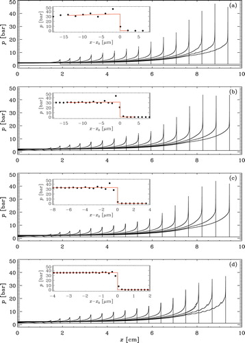
Table 1. Summary of the fit parameters at $t=42\text{μ}\mathrm{s}$; $x_0$ is in cm, $p_0$ and $p_1$ are in bar, $p_1^{\prime }$ is in $\mathrm{bar}\text{μ}{\mathrm{m}}^{-1}$, $L_1$ and $L_2$ are in $\text{μ}\mathrm{m}$, and $\delta t_{min}$ in $\mathrm{ps}$.

	$\delta x$	$x_0$	$p_1$	$p_1^{\prime }$	$L_1$	$L_2$	$N_x$	$N_t$	$\delta t_{min}$
(a)	1.993	9.37498	35.00	0.2200	2.56	0.36	50,176	392,000	42
(b)	0.997	9.44825	31.20	0.0546	1.21	0.30	100,352	1,266,600	24
(c)	0.498	9.44390	33.21	0.0535	0.442	0.0587	200,704	2,826,300	12
(d)	0.199	9.27530	35.78	0.1128	0.1145	0.0157	501,760	14,603,000	2.5
(e)	0.199	9.46444	28.70	0.0300	0.4069	0.1719	501,760	14,255,800	2.5

Note: Runs (a–d) have $C_{\mathrm{shock}}=0.8$ and run (e) has $C_{\mathrm{shock}}=0.2$.

It is evident that the wiggles decrease as we increase the resolution. In addition, the pressure profiles change slightly with resolution. To characterise these changes, we determine a fit to the pressure peak of the form (21) $p_{\mathrm{fit}}(x,t_{\ast })=p_0+[p_1+(x-x_0)p_1^{\prime }]\Theta (x_0-x),$(21) where $\Theta (x)$ is the Heaviside step function ($=1$ for x>0 and zero otherwise), $x_0$ is the position of the peak at the last time $t_{\ast }$, $p_0$ is the atmospheric background pressure ahead of the peak, $p_1$ is the pressure increase relative to $p_0$ just behind the peak, and $p_1^{\prime }$ is the slope of the pressure profile to the left of the peak, i.e. in the wake of the detonation wave. In all cases, the pressure ahead of the peak is $p_0=1.013\times {10}^6\mathrm{dyn}{\mathrm{cm}}^{-2}$, which does not need to be fitted. The remaining three parameters are given in table 1, where the pressure is given in bar ($1\mathrm{bar}={10}^6\mathrm{dyn}{\mathrm{cm}}^{-2}$).

Note that between the runs with $\delta x=1\text{μ}\mathrm{m}$ and $0.5\text{μ}\mathrm{m}$, the front speeds (or front positions $x_0$) agree within 0.05%, but for the run with $\delta x=0.2\text{μ}\mathrm{m}$, the front speed has decreased by nearly 2%. The reason for this apparent loss of accuracy is not fully identified, although it is clear that smaller values of $C_{\mathrm{shock}}$ lead again to larger front speeds; see run (e) in table 1. It is therefore possible that at this high resolution, the value $C_{\mathrm{shock}}=0.8$ is already too large and that a smaller value, for example around 0.6, could be more reasonable. We should also point out that we have used a relatively optimistic choice of the viscous time step (we chose $\delta t{\nu }_{max}/\delta x^2=0.4$ instead of the more conservative value of 0.25 that is recommended in the manual to the PENCIL CODE). However, comparisons with the smaller value did not indicate any differences in the front speed. The fact that the viscous time step enters in this highest resolution run, but not in the others, is related to the extremely small mesh size in this case. This makes the time step constraint from the relatively large molecular viscosity near x = 0 very severe. Note also that in this run, waves appear in the wake of the pressure field behind the peak after $t=36\text{μ}\mathrm{s}$. These also seem to be spurious and are not found when $C_{\mathrm{shock}}$ is smaller.

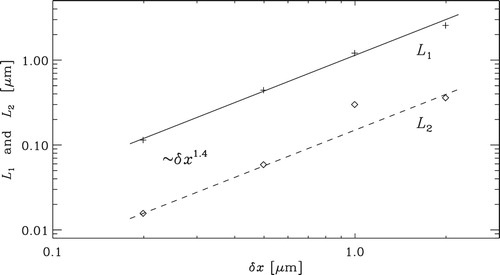
Next, to characterise the convergence, we use the $L_1$ and $L_2$ norms defined here as follows: (22) $\begin{array}{rl}{L}_1& ={\int }_{x_1}^{x_2}|p(x,t_{\ast })-p_{\mathrm{fit}}(x,t_{\ast })|\mathrm{d}x/(p_0+p_1),\end{array}$(22) (23) $\begin{array}{rl}{L}_2& ={\int }_{x_1}^{x_2}{|p(x,t_{\ast })-p_{\mathrm{fit}}(x,t_{\ast })|}^2\mathrm{d}x/(p_0+p_1{)}^2.\end{array}$(23) Both have the dimension of a length. These values are also given in table 1. Figure 2 shows that $L_1$ and $L_2$ decrease with resolution like $\delta x^{1.4}$.

Figure 2. Convergence of $L_1$ and $L_2$ with $\delta x$.

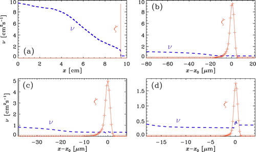
In figure 3 we compare the molecular viscosity profile at the last time with the corresponding shock viscosity for the three highest resolutions shown in figure 1(b–d). The overall profile of the molecular viscosity is the same in all three cases and varies significantly from $\sim 10{\mathrm{cm}}^2{\mathrm{s}}^{-1}$ at x = 0 to $\sim 0.3{\mathrm{cm}}^2{\mathrm{s}}^{-1}$ at and ahead of the shock. However, the peak of the shock viscosity decreases from $\sim 10{\mathrm{cm}}^2{\mathrm{s}}^{-1}$ in figure 1(b) by about a factor of five to $\sim 1.8{\mathrm{cm}}^2{\mathrm{s}}^{-1}$ in figure 1(d). In addition, the width of the shock viscosity profile also decreases by about a factor of five, so the integrated effect of the shock viscosity diminishes by a factor of about 25, as expected from equation (17(17) $\zeta =C_{\mathrm{shock}}\delta x^2⟨-\mathbf{\nabla }\mathbf{\cdot }\mathit{U}{⟩}_{+},$(17) ). Note that for the highest resolution, the shock viscosity makes up a small contribution compared to the molecular viscosity. We emphasise that the maximum of the molecular viscosity ($\sim 10{\mathrm{cm}}^2{\mathrm{s}}^{-1}$ at x = 0) is much larger than the maximum of the shock viscosity ($\sim 1.8{\mathrm{cm}}^2{\mathrm{s}}^{-1}$ at $x=9.4\mathrm{cm}$, although at this point the molecular value is only $\sim 0.3{\mathrm{cm}}^2{\mathrm{s}}^{-1}$); compare figure 3(a,d). This means that at late times, when ν has become large far in the wake of the shock, an enormous amount of time is spent because the viscous time step is then so short. This is also evident from table 1, where we see that the total number of time steps has increased by a factor of over five as the resolution was increased by only a factor of 2.5.

Figure 3. Comparison of the profiles of viscosity (ν, blue dashed lines) and shock viscosity (ζ, red lines with mesh points being marked with plus signs) for (a) $\delta x=1\text{μ}\mathrm{m}$ showing the full x range from 0 to $10\mathrm{cm}$. (b)–(d) show only the close proximity of the shock at $x_0$ for (b) $\delta x=1\text{μ}\mathrm{m}$, (c) $\delta x=0.5\text{μ}\mathrm{m}$, and (d) $\delta x=0.2\text{μ}\mathrm{m}$, at $t=42\text{μ}\mathrm{s}$ (colour online).

3.3. Dependence on $C_{\mathrm{shock}}$

Next, we investigate the dependence of our solutions on the value of $C_{\mathrm{shock}}$. In figure 4 we show pressure profiles for different values of $C_{\mathrm{shock}}$ at resolutions of $\delta x=1\text{μ}\mathrm{m}$ and $0.5\text{μ}\mathrm{m}$. For $C_{\mathrm{shock}}\le 1.4$, the pressure profiles still show wiggles at the position of the pressure maximum, but the wiggles are smaller and more localised at the higher resolution of $0.5\text{μ}\mathrm{m}$. For $C_{\mathrm{shock}}=1.4$, however, the wiggles are nearly completely negligible at the resolutions of $0.5\text{μ}\mathrm{m}$, but the pressure profile has also changed in that case and has now a short flank with a negative slope just behind the shock, that is, to its left. For $C_{\mathrm{shock}}=1.5$, TD is only found in the case with $\delta x=1\text{μ}\mathrm{m}$, but not with $\delta x=0.5\text{μ}\mathrm{m}$.

In figure 5, we show a larger portion of the wake behind the pressure front, where we see the occurrence of another type of long-wavelength oscillation, when $C_{\mathrm{shock}}$ is larger than 0.8. Those waves are similar for both the higher and lower resolution runs, but could also be a feature of having under-resolved the solution at earlier times that are not shown here.

Figure 4. Comparison of pressure and temperature profiles for $C_{\mathrm{shock}}=0.8$ (black), 1.0 (red), 1.2 (orange), 1.4 (green), and 1.5 (blue), for $\delta x=1\text{μ}\mathrm{m}$ (top) and $0.5\text{μ}\mathrm{m}$ (bottom). Note that for $C_{\mathrm{shock}}=1.5$ and $\delta x=0.5\text{μ}\mathrm{m}$, no TD develops (colour online).

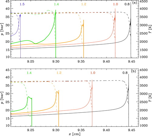
Figure 5. Similar to figure 4, but showing also the wake of the pressure front. Note the waves in the simulations with $C_{\mathrm{shock}}>0.8$; see the blue, green, orange, and red lines (colour online).

3.4. Speeds of pressure and reaction fronts

Finally, we show in figure 6 the time dependence of the positions and speeds of the pressure and spontaneous reaction fronts. In practice, the speeds $U_i$ (with $i=\mathrm{p}$ for pressure and $i=\mathrm{sp}$ for spontaneous reaction wave) are computed by time differentiation of the position $x_i$, which is obtained from the volume where the pressure or the reactant are above a certain threshold. Specifically, we compute (24) $U_{\mathrm{p}}=\frac{\mathrm{d}{x}_{\mathrm{p}}}{\mathrm{d}t}=-\frac{\mathrm{d}}{\mathrm{d}t}{\int }_0^{x_{max}}max(p_{\mathrm{crit}}-p,0)/(p_{\mathrm{crit}}-p_0)\mathrm{d}x,$(24) where we have used $p_{\mathrm{crit}}=1.020\mathrm{bar}$ as threshold pressure and $p_0=1.013\mathrm{bar}$ is still the same background pressure as in equation (21(21) $p_{\mathrm{fit}}(x,t_{\ast })=p_0+[p_1+(x-x_0)p_1^{\prime }]\Theta (x_0-x),$(21) ). The spontaneous reaction speed is based on the amount of water produced, i.e. (25) $U_{\mathrm{sp}}=\frac{\mathrm{d}{x}_{\mathrm{sp}}}{\mathrm{d}t}=-\frac{\mathrm{d}}{\mathrm{d}t}{\int }_0^{x_{max}}max(1-Y_k/Y_{k0},0)\mathrm{d}x,$(25) where $k={\mathrm{H}}_2\mathrm{O}$ and $Y_{k0}=0.3$ is half the value of $Y_k\approx 0.6$ after ${\mathrm{H}}_2$ has reacted with ${\mathrm{O}}_2$. The final values of the two speeds are $U_{\mathrm{p}}=3.06\mathrm{km}{\mathrm{s}}^{-1}$ and $U_{\mathrm{sp}}=3.01\mathrm{km}{\mathrm{s}}^{-1}$. These values are close to the empirically determined value of $3.0\mathrm{km}{\mathrm{s}}^{-1}$, which is only known to within about 1% accuracy and therefore compatible with our results.

Figure 6. Front positions and speeds for $\delta x=0.5\text{μ}\mathrm{m}$ and $C_{\mathrm{shock}}=0.8$. (a) $x_{\mathrm{sp}}(t)$ (red solid line) and $x_{\mathrm{p}}(t)$ (blue dashed line), (b) $U_{\mathrm{sp}}(t)$ (red solid line) and $U_{\mathrm{p}}(t)$ (blue dashed line), and (c) $U_{\mathrm{sp}}(x)$ (red solid line) and $U_{\mathrm{p}}(x)$ (blue dashed line) (colour online).

According to equation (19(19) $U_{\mathrm{sp}}=\frac{\mathrm{d}x}{\mathrm{d}{\tau }_{\mathrm{ind}}}={\left(\frac{\mathrm{d}{\tau }_{\mathrm{ind}}}{\mathrm{d}T}\right)}^{-1}{\left(\frac{\mathrm{d}T}{\mathrm{d}x}\right)}^{-1}$(19) ), the velocity of the spontaneous reaction wave decreases in the beginning, since $U_{\mathrm{sp}}\propto (\mathrm{d}{\tau }_{\mathrm{ind}}/\mathrm{d}T{)}^{-1}$. It reaches a minimum somewhere near the crossover temperature $T_{\mathrm{cr}}\approx 1000\mathrm{K}$ (for the present mixture of ${\mathrm{H}}_2$ and ${\mathrm{O}}_2$) for the steepest gradient capable of initiating detonation which corresponds to the transition from the endothermal to the exothermal stage of the reaction. In our case, the gradient is rather shallower, so the minimum of the velocity is reached earlier.

After reaching the minimum velocity, the speed of the spontaneous reaction wave increases due to energy release in the reaction. To accomplish coupling between the spontaneous reaction wave and the pressure wave, it is necessary (but not sufficient) that $U_{\mathrm{sp}}>U_{\mathrm{p}}$ after the point where $U_{\mathrm{sp}}$ is minimum, which is the case during the interval $12\text{μ}\mathrm{s}\le t\le 19\text{μ}\mathrm{s}$. For $t>19\text{μ}\mathrm{s}$, the coupling between the reaction wave and the shock wave is developing until detonation is reached at $t\approx 38\text{μ}\mathrm{s}$. Note also that $U_{\mathrm{sp}}$ is now slightly less than $U_{\mathrm{p}}$, but this is natural because the reaction happens always slightly behind the leading shock. In fact, at late times, hardly any difference between $x_{\mathrm{p}}$ and $x_{\mathrm{sp}}$ can be seen; see figure 6(a). This is compatible with the experimental value of the detonation; see Kuznetsov et al. (2005).

4. Comparison with the WENO code

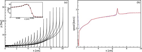
There is extensive literature devoted to the simulation of hydrodynamic problems with shock and detonation waves using a shock-capturing approach (Cai et al. 2018, Deng et al. 2018, 2019, Zhao et al. 2018, Dong et al. 2019, Fan et al. 2019, Huang and Shu 2019). In this section we consider solutions to the detonation problem (see section 2.2 for details) using the WENO code, which is widely used to simulate various combustion and detonation problems. Compared to the results obtained with the PENCIL CODE, there are no wiggles in the pressure profiles without the addition of a shock viscosity due to the usage of the WENO scheme. Figure 7(a) shows the evolution of pressure profiles during the formation of a steady detonation after the coupling of the spontaneous reaction and shock waves has been obtained in the simulations with the WENO code at resolution $\delta x=10\text{μ}\mathrm{m}$. The corresponding spontaneous reaction wave velocity and pressure wave velocity are presented in figure 7(b). Small oscillations of the velocities of the reaction and pressure waves indicate the coupling of shock and spontaneous reaction waves in the beginning of the development toward detonation. However, the simulations shown in figure 8 at a higher resolution with $\delta x=5\text{μ}\mathrm{m}$ show that the developing detonation quenches before it leaves the temperature gradient. The previously successfully coupled reaction and shock waves are decoupled at around $7.4\mathrm{cm}$. It is worth noting that the quenching of detonation in this case is in no way due to the gradient being too steep. Simulations with a resolution of $\delta x=5\text{μ}\mathrm{m}$ for a much shallower gradient ($L=18\mathrm{cm}$) also show that the initially coupled reaction and shock waves later decouple and the initially developing detonation quenches.

Figure 7. (a) pressure profiles calculated with the WENO code at resolution $\delta x=10\text{μ}\mathrm{m}$, in regular time intervals from $0\text{μ}\mathrm{s}$ to $46\text{μ}\mathrm{s}$. The inset shows the vicinity of the pressure peak at $42\text{μ}\mathrm{s}$. (b) corresponding spontaneous wave velocity (red solid line) and pressure wave velocity; see the blue dashed line (colour online).

Figure 8. Similar to figure 7, but for $\delta x=5\text{μ}\mathrm{m}$ and without inset (colour online).

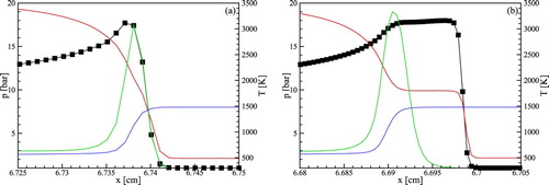
Figure 9(a,b) show profiles of pressure, temperature, and mass fractions of $\mathrm{H}{\mathrm{O}}_2$ and ${\mathrm{H}}_2$ at $t=34\text{μ}\mathrm{s}$, calculated using the WENO scheme at resolutions $\delta x=10\text{μ}\mathrm{m}$ and $\delta x=5\text{μ}\mathrm{m}$. It is seen that, without artificial viscosity, the width of the shock is too small at a resolution of $\delta x=5\text{μ}\mathrm{m}$ so that the coupling of the reaction and shock waves becomes impossible, resulting in a quenching of the detonation, as shown in figure 8. While the non-oscillating shock-capturing WENO scheme works quite well for simulations of hydrodynamic problems with shock waves, it does not work for the problem of detonation development, which is more “sensitive to the resolution” compared to ordinary supersonic flows with shock waves. The solution obtained with the WENO scheme at a low resolution in figure 7 ($\delta x=10\text{μ}\mathrm{m}$) shows the development of a steady detonation, but at the higher resolution of figure 8 ($\delta x=5\text{μ}\mathrm{m}$), the shock becomes too thin (figure 9), and thus could not couple with the reaction wave, so the detonation quenches.

Figure 9. Profiles of pressure (black line), temperature (red line), mass fraction of $\mathrm{H}{\mathrm{O}}_2$ (green line), and ${\mathrm{H}}_2$ (blue line) at $t=34\text{μ}\mathrm{s}$, calculated with the WENO code at resolutions $\delta x=10\text{μ}\mathrm{m}$ (a) and $\delta x=5\text{μ}\mathrm{m}$ (b) (colour online).

The physical problem in question, also known as the shock wave amplification by coherent energy release (SWACER) mechanism, which is a particular case of a detonation initiated by shallow temperature (or reactivity) gradients, has been studied experimentally by Lee et al. (1978). In this case, the shock-capturing approach of WENO does not work. More precisely, it works only at low resolutions, here with $\delta x=10\text{μ}\mathrm{m}$, when the width of the shock, obtained with WENO, is sufficiently large for coupling of pressure wave and the subsequent shock with the spontaneous reaction wave. In simulation of the SWACER problem, shock-capturing and artificial viscosities (numerical dissipation) must be compatible with the size of the computation resolution in the sense that, if the reaction wave was coupled with the pressure wave and later with the shock wave, it must remain coupled with the shock at all times until a strong shock wave is formed and then develops into a steady detonation.

We use the artificial viscosity developed by Kurganov and Liu (2012) to increase the numerical dissipation of the WENO scheme. This does not contradict to the definition of convergence, because the artificial viscosity tends to zero, as $\delta x$ tends to zero. At the same resolution, however, the numerical dissipation of the WENO scheme with artificial viscosity is larger than that of the WENO scheme. The simulation with the WENO code with artificial viscosity for a resolution of $\delta x=5\text{μ}\mathrm{m}$ results in the development of a steady detonation, as shown in figure 10. In simulations of problems containing shocks, we can calibrate the parameter of the artificial viscosity for a low resolution, but the problem of detonation development (SWACER) is special, because in this case the parameter of artificial viscosity depends on the resolution, which makes the simulations much more demanding and time consuming, especially when we use detailed chemical models.

Figure 10. Similar to figure 7, but for $\delta x=5\text{μ}\mathrm{m}$ and with artificial viscosity (colour online).

It should be noted that the minimum resolution at which WENO code allows us to obtain a solution to the SWACER problem depends on the particular combustion gas mixture, the chemical kinetics scheme, and the initial pressure. At high resolution, the WENO code without artificial viscosity still shows the development of steady detonation for the mixture with high initial pressure. For example, for an initial pressure of 5 bar, a steady detonation develops for the largest resolution of about $\delta x=2\text{μ}\mathrm{m}$ without the use of artificial viscosity.

5. Conclusions

Using high-resolution simulations of detonation initiated by an initial temperature gradient in a hydrogen–oxygen mixture, we have shown, using the PENCIL CODE, that the transition to and properties of detonation can successfully be modelled for intermediate values of the shock viscosity parameter. The numerical error, as determined by comparing with an empirical fit to the pressure peak in the final stage of TD, is found to decrease like $\delta x^{1.4}$ with decreasing mesh size down to $\delta =0.2\text{μ}\mathrm{m}$. (The typical performance is $0.05\text{μ}\mathrm{s}$ wall clock time per step and mesh point with 2048 processors on a Cray XC40 with $2.3\mathrm{GHz}$ Intel cores.) The shock viscosity has non-vanishing values only in the immediate proximity of the shock and reaches there still values of about four times the molecular value in our highest resolution simulation. Unfortunately, the position of the shock still depends on the value of $C_{\mathrm{shock}}$ of around $3\mathrm{km}{\mathrm{s}}^{-1}$. Nevertheless, the shock speed reaches the expected value in the final stage of TD.

It remains unsatisfactory that even at the largest resolution of half a million mesh points in just the x direction, we are still unable to avoid the use of a shock viscosity. This is because the shock is so strong and the molecular viscosity still too small by comparison. Furthermore, we have been unable to demonstrate that the use of a small amount of shock viscosity does not affect the details of the shock position or even the detailed shape of the shock profile. We can therefore not be completely sure that TD will still be recovered at even higher resolution, which has not yet been possible to simulate. A reason for the current limitation is that our code is optimised to work for three-dimensional problems. It is therefore conceivable that a significant speed-up could be achieved by optimising the code for one-dimensional problems. In that case it would also be rather straightforward to use an adaptive mesh, which could make the calculations significantly more economic.

Another possible avenue for future research is to solve the governing equations in conservative form so that mass, momentum, and energy are conserved to machine precision. A difficulty here is the presence of source terms in the equations for the mass fractions of the individual species.

The WENO scheme is computationally demanding and it is difficult to reach resolutions comparable to what has been done with the PENCIL CODE. Nevertheless, a steady detonation front was obtained at the resolution of $\delta x=10\text{μ}\mathrm{m}$, and with the use of artificial viscosity at the resolution $\delta x=5\text{μ}\mathrm{m}$. On the other hand, of course, we know from experiments that TD does occur. Thus, assuming that our equations are physically correct, as stated, there should be no doubt that any failure to recover TD must be regarded as a numerical artifact.

Yet another approach is to isolate the essence of the problem in a simpler single reaction model. One must then also use an idealised viscosity and a simplified equation of state. Those modifications could enable us to perform simulations at much higher resolution so that it is possible to focus on the purely numerical aspect of using a shock viscosity in this problem.

Acknowledgments

Simulations presented in this work have been performed with computing resources provided by the Swedish National Allocations Committee at the Center for Parallel Computers at the Royal Institute of Technology in Stockholm.

Disclosure statement

No potential conflict of interest was reported by the authors.

ORCID

Chengeng Qian http://orcid.org/0000-0002-5560-5475

Axel Brandenburg http://orcid.org/0000-0002-7304-021X

Mikhael A. Liberman http://orcid.org/0000-0003-4308-7225

Additional information

Funding

This research was supported in part by the National Key R&D Program of China (Grant No. 2018YFC0807900), the National Natural Science Foundation of China (grant 11732003), the Beijing Natural Science Foundation (grant 8182050), the National Science Foundation under the Astronomy and Astrophysics Grants Program (grant 1615100), and the University of Colorado through its support of the George Ellery Hale visiting faculty appointment.

References

- Babkovskaia, N., Haugen, N.E.L. and Brandenburg, A., A high-order public domain code for direct numerical simulations of turbulent combustion. J. Comp. Phys. 2011, 230, 1–12. doi: 10.1016/j.jcp.2010.08.028
- Bartenev, A. and Gelfand, B., Spontaneous initiation of detonations. Prog. Energy Combust. Sci. 2000, 26, 29–55. doi: 10.1016/S0360-1285(99)00007-6
- Bates, L., Bradley, D., Paczko, G. and Peters, N., Engine hot spots: Modes of auto-ignition and reaction propagation. Combust. Flame 2016, 166, 80–85. doi: 10.1016/j.combustflame.2016.01.002
- Bradley, D. and Kalghatgi, G.T., Influence of autoignition delay time characteristics of different fuels on pressure waves and knock in reciprocating engines. Combust. Flame 2009, 156, 2307–2318. doi: 10.1016/j.combustflame.2009.08.003
- Bradley, D., Autoignitions and detonations in engines and ducts. Phil. Trans. Roy. Soc. A 2012, 370, 689–714. doi: 10.1098/rsta.2011.0367
- Cai, Y., Ao, Y., Yang, C., Ma, W. and Zhao, H., Extreme-scale high-order WENO simulations of 3-D detonation wave with 10 million cores. ACM T. Archit. Code Op. 2018, 15, 26.
- Coffee, T.P. and Heimerl, J.M., Transport algorithms for premixed, laminar steady-state flames. Combust. Flame 1981, 43, 273–289. doi: 10.1016/0010-2180(81)90027-4
- Dai, P. and Chen, Z., Supersonic reaction front propagation initiated by a hot spot in n-heptane/air mixture with multistage ignition. Combust. Flame 2015, 162, 4183–4193. doi: 10.1016/j.combustflame.2015.08.002
- Dai, P., Chen, Z., Chen, S. and Ju, Y., Numerical experiments on reaction front propagation in n-heptane/air mixture with temperature gradient. Proc. Combust. Inst. 2015, 35, 3045–3052. doi: 10.1016/j.proci.2014.06.102
- Deng, X., Xie, B., Loubère, R., Shimizu, Y. and Xiao, F., Limiter-free discontinuity-capturing scheme for compressible gas dynamics with reactive fronts. Comput. Fluids 2018, 171, 1–14. doi: 10.1016/j.compfluid.2018.05.015
- Deng, X., Xie, B., Teng, H. and Xiao, F., High resolution multi-moment finite volume method for supersonic combustion on unstructured grids. Appl. Math. Model. 2019, 66, 404–423. doi: 10.1016/j.apm.2018.08.010
- Dong, H., Fu, L., Zhang, F., Liu, Y. and Liu, J., Detonation simulations with a fifth-order teno scheme. Commun. Comput. Phys. 2019, 25, 1357–1393. doi: 10.4208/cicp.OA-2018-0008
- Evlampiev, A., Numerical Combustion Modeling for Complex Reaction Systems, Vol. 68/04, 2007 (Eindhoven Techn. Univ.: Eindhoven).
- Fan, W., Zhong, F., Ma, S. and Zhang, X., Numerical study of convective heat transfer of supersonic combustor with varied inlet flow conditions. Acta Mech. Sin. 2019, doi: 10.1007%2Fs10409-019-00882-x
- Gottlieb, S., Shu, C.W. and Tadmor, E., Strong stability-preserving high-order time discretization methods. SIAM Rev. 2001, 43, 89–112. doi: 10.1137/S003614450036757X
- Gu, X.J., Emerson, D.R. and Bradley, D., Modes of reaction front propagation from hot spots. Combust. Flame 2003, 133, 63–74. doi: 10.1016/S0010-2180(02)00541-2
- He, L., Theoretical determination of the critical conditions for the direct initiation of detonations in hydrogen-oxygen mixtures. Combust. Flame 1996, 104, 401–418. doi: 10.1016/0010-2180(96)00141-1
- He, L. and Clavin, P., Critical conditions for detonation initiation in cold gaseous mixtures by nonuniform hot pockets of reactive gases, Twenty-Fourth Symposium on Combustion, University of Sydney, Sydney, Australia, Vol. 24, 1992, pp. 1861–1867.
- Huang, J. and Shu, C.W., Positivity-preserving time discretizations for production–destruction equations with applications to non-equilibrium flows. J. Sci. Comput. 2019, 78, 1811–1839. doi: 10.1007/s10915-018-0852-1
- Jiang, G. and Shu, C., Efficient implementation of weighted ENO schemes. J. Comput. Phys. 1996, 126, 202–228. doi: 10.1006/jcph.1996.0130
- Kéromnès, A., Metcalfe, W.K., Heufer, K.A., Donohoe, N., Das, A.K., Sung, C.J., Herzler, J., Naumann, C., Griebel, P., Mathieu, O., Krejci, M.C., Petersen, E.L., Pitz, W.J. and Curran, H.J., An experimental and detailed chemical kinetic modeling study of hydrogen and syngas mixture oxidation at elevated pressures. Combust. Flame 2013, 160, 995–1011. doi: 10.1016/j.combustflame.2013.01.001
- Khokhlov, A., Oran, E. and Wheeler, J., A theory of deflagration-to-detonation transition in unconfined flames. Combust. Flame 1997, 108, 503–517. doi: 10.1016/S0010-2180(96)00105-8
- Kurganov, A. and Liu, Y., New adaptive artificial viscosity method for hyperbolic systems of conservation laws. J. Comput. Phys. 2012, 231, 8114–8132. doi: 10.1016/j.jcp.2012.07.040
- Kurtz, M.D. and Regele, J.D., Acoustic timescale characterisation of a one-dimensional model hot spot. Combust. Theory Model. 2014, 18, 532–551. doi: 10.1080/13647830.2014.934922
- Kuznetsov, M., Alekseev, V., Matsukov, I. and Dorofeev, S., DDT in a smooth tube filled with a hydrogen oxygen mixture. Shock Waves 2005, 14, 205–215. doi: 10.1007/s00193-005-0265-6
- Lee, J. and Moen, I., The mechanisms of transition from deflagration to detonation in vapor cloud explosions. Prog. Energ. Combust. Sci. 1980, 6, 359–389. doi: 10.1016/0360-1285(80)90011-8
- Lee, J., Knystautas, R. and Yoshikawa, N., Photochemical initiation of gaseous detonations. Acta Astronaut. 1978, 5, 971–982. doi: 10.1016/0094-5765(78)90003-6
- Liberman, M.A., Kiverin, A.D. and Ivanov, M.F., On detonation initiation by a temperature gradient for a detailed chemical reaction models. Phys. Lett. A 2011, 375, 1803–1808. doi: 10.1016/j.physleta.2011.03.026
- Liberman, M.A., Kiverin, A. and Ivanov, M., Regimes of chemical reaction waves initiated by nonuniform initial conditions for detailed chemical reaction models. Phys. Rev. E 2012, 85, 056312. doi: 10.1103/PhysRevE.85.056312
- Liberman, M.A., Wang, C., Qian, C. and Liu, J., Influence of chemical kinetics on spontaneous waves and detonation initiation in highly reactive and low reactive mixtures. Combust. Theory Model. 2019, 23, 467–495. doi: 10.1080/13647830.2018.1551578
- Lo, S.C., Blaisdelly, G.A. and Lyrintzisz, A.S., High-order shock capturing schemes for turbulence calculations, in 45th AIAA Aerospace Sciences Meeting and Exhibit, Reno, Nevada, January 8–11, 2007, 2007, pp. 1–18.
- Mourits, M.M. and Rummens, F.H.A., A critical evaluation of Lennard-Jones and Stockmayer potential parameters and of some correlation methods. Can. J. Chem. 1977, 55, 3007–3020. doi: 10.1139/v77-418
- Poinsot, T. and Veynante, D., Theoretical and Numerical Combustion, 2005 (RT Edwards, Inc. Philadelphia, USA).
- Rudloff, J., Zaccardi, J.M., Richard, S. and Anderlohr, J., Analysis of pre-ignition in highly charged SI engines: Emphasis on the auto-ignition mode. Proc. Combust. Inst. 2013, 34, 2959–2967. doi: 10.1016/j.proci.2012.05.005
- von Neumann, J. and Richtmyer, R.D., A method for the numerical calculation of hydrodynamic shocks. J. Appl. Phys. 1950, 21, 232–237. doi: 10.1063/1.1699639
- Wang, C., Qian, C., Liu, J. and Liberman, M.A., Influence of chemical kinetics on detonation initiating by temperature gradients in methane/air. Combust. Flame 2018, 197, 400–415. doi: 10.1016/j.combustflame.2018.08.017
- Wilke, C.R., A viscosity equation for gas mixtures. J. Comp. Phys. 1950, 18, 517–519.
- Zeldovich, Y.B., Regime classification of an exothermic reaction with nonuniform initial conditions. Combust. Flame 1980, 39, 211–214. doi: 10.1016/0010-2180(80)90017-6
- Zeldovich, Y., Librovich, V., Makhviladze, G. and Sivashinsky, G., On the development of detonation in a non-uniformly preheated gas. Acta Astron. 1970, 15, 313–321.
- Zeldovich, Y.B., Gelfand, B., Tsyganov, S., Frolov, S. and Polenov, A., Concentration and temperature nonuniformities of combustible mixtures as reason for pressure waves generation. Dyn. Explosions 1988, 114, 99.
- Zhao, W.G., Zheng, H.W., Liu, F.J., Shi, X.T., Gao, J., Hu, N., Lv, M., Chen, S.C. and Zhao, H.D., An efficient unstructured WENO method for supersonic reactive flows. Acta Mech. Sin. 2018, 34, 623–631. doi: 10.1007/s10409-018-0756-1