Instabilities and vertical mixing in river plumes: application to the Bay of Biscay

Abstract

In the Bay of Biscay (north-east Atlantic), long-living eddies and the frontal activity that they induce substantially contribute to mesoscale and submesoscale dynamics. Tides and river plumes also contribute to frontal activity. Biological productivity is sensitive to river plume fronts and to external forcings (tides and wind). Considering the importance of river plumes, we study here the structure, stability and vertical mixing processes in such river plumes (similar to those generated by the Gironde river). Restratification budget is considered here for evaluating stirring (frontogenetic/frontolytic) or vertical mixing (parametrised here from Ertel potential vorticity mixing) processes. Using high-resolution idealised numerical simulations, we analyse the evolution of the bulge and of the coastal part of this plume and we conduct sensitivity experiments to the river discharge, to southwesterly winds and to M2 tides. The bulge and the coastal current are stable (unstable) in case of moderate (high) river discharge, due to mixed barotropic/baroclinic instabilities. In the unstable case, near surface symmetric and vertical shear instabilities develop in the coastal current and in the core of the bulge where the Rossby number is large. When southwesterly winds blow, the river plume is squeezed near the coast by Ekman transport. The river plume is then subject to frontal symmetric, baroclinic, barotropic and vertical shear instabilities in the coastal part, north of the estuary (its far field). Conversely, in the presence of M2 tides, the river plume is barotropically, baroclinically and symmetrically unstable in its near field. Interior vertical mixing is induced by advective (stirring) and frontogenetic processes. Frontogenesis is dominant in the far-field (in the presence of southwesterlies) or in the near-field (when M2 tide is active). Frontogenesis is important in the far-field region in unforced river plumes (both with moderate and high river discharges). Potential vorticity is eroded in the far-field when southwesterlies blow. This is primarily due to the frictional processes which are dominant at the surface. This study has identified the instabilities which affect a river plume in different cases, and the local turbulent processes which alter the stratification.

Keywords:

• River plumes
• Gironde river
• (sub)mesoscale instabilities
• vertical mixing
• stratification

1. Introduction

Over the last decades, there has been a growing interest in the Bay of Biscay for economic and scientific reasons. This semi-enclosed region is recognised for multiple oceanographic features: as part of the north-east Atlantic Ocean, it is influenced by a general anticyclonic circulation in the open ocean and by a poleward flow over the shelf break, the Iberian poleward slope current (IPC) (Pingree and Le Cann 1990, Charria et al. 2013, Teles-Machado et al. 2015). The circulation in the Bay of Biscay is also forced by northwesterly and southwesterly winds, moderate tides, or seasonal river discharges. These forcings drive coastal currents, upwellings and downwellings and vertical mixing of the water masses.

Over the shelf-break and in the deep ocean, mesoscale activity is manifested in long living quasi-stationary anticyclonic eddies in northern Spain, and in the central basin, respectively, called 4${}^{\circ }$W eddy and slope water oceanic eddies (SWODDIES) (Pingree and Sinha 2001, Caballero et al. 2014). The IPC perturbations mainly result in the generation of these strong eddies. When they are not trapped by topography, the 4${}^{\circ }$W eddy and SWODDIES are, respectively, driven by density forcing and they are advected to the west. The slope water oceanic eddies have typical migration speeds of $2\mathrm{cm}{\mathrm{s}}^{-1}$ comparable with long Rossby waves phase speed ($\beta R_d^2$ with $\mathrm{Rd}=25-30\mathrm{km}$ the Rossby radius of deformation in the abyssal plain and $\beta =1.5\times {10}^{-11}{\mathrm{m}}^{-1}{\mathrm{s}}^{-1}$) (Pingree and Sinha 2001, Caballero et al. 2014). A warm anticyclone, generated over the shelf-break after wind relaxation and drifting northwards after several weeks, has been observed using high-frequency radar data (Rubio et al. 2018). The eddies mentioned above have similar characteristics: a radius of 25–50 km, a vertical extent ranging from 100 m to 2 km and a rotation period between 7 h and 3.5 days. The 4${}^{\circ }$W eddy and SWODDIES have lifetimes, respectively, of about seven months and one year (Pingree and Sinha 2001, Caballero et al. 2014).

In the shallower region over the continental shelf, the Bay of Biscay is characterised by two main riverine inputs (the Loire and the Gironde rivers). These two rivers provide a noticeable runoff in the bay, with an annual average discharge of $900{\mathrm{m}}^3{\mathrm{s}}^{-1}$ each (Lazure et al. 2009). Obviously, this discharge is small compared to those of the Columbia or of the Mississippi rivers ($\mathrm{10,000}{\mathrm{m}}^3{\mathrm{s}}^{-1}$ and $\mathrm{30,000}{\mathrm{m}}^3{\mathrm{s}}^{-1}$). The Columbia and Mississippi river plumes are subject to tide and wind-driven dynamics, respectively, comparable to Gironde river plume. Indeed, the Columbia river plume is subject to tide stirring and mixing in its near field where many fronts are formed (Kilcher and Nash 2010). On the other hand, the Mississippi river plume is subject to Eastward wind-driven currents which alter its far-field and exhibit a large freshwater transport toward the shelf break and the DeSoto Canyon (Schiller et al. 2011). Therefore, the Gironde river can be considered as a river system where both effects (wind and tides) can be analysed in a single region. When the river flow enters the coastal ocean, the expansion of the plume in the near field is linked to the river discharge: the momentum of the plume layer dominates its buoyancy (Horner-Devine et al. 2015). Conversely, the Coriolis force brings the plume back along the coast (to the right of the plume in the Northern Hemisphere). At the river mouth, and for weak wind forcing, this plume curvature can create an anticyclonic bulge; the bulge radius can grow up to a few internal Rossby radii (Garvine 1999). The plume characteristics depend on the relative influences of the stratification created by the freshwater discharge and its mixing with the ambient, saline waters. Near the estuary (in the near field of the plume), this mixing is governed by the flow acceleration, by variable advection and by turbulent processes (Horner-Devine et al. 2015). In the far-field region of the plume, the wind influence dominates the mixing processes (Fong and Geyer 2001). Tides can also affect river plumes. Flood-ebb tidal straining generates periodic fluctuations of the density stratification (Simpson et al. 1990, Isobe 2005, Iwanaka and Isobe 2018); conversely, this stratification alters the tidal currents (Visser et al. 1994, Li and Rong 2012).

Based on O'Donnell definition, in the absence of wind an along-shore coastal current forms. The vertical structure of this coastal current is delimited by a plume front (offshore extent of buoyant water). The plume front encounters the bottom at a location called “the inshore edge of the frontal zone .” From this specific location, inshore and offshore regions are formed as sketched in figure 8.10(c) in (O'Donnell 2010) and as defined in Lentz and Largier (2006). The ratio of the areas of those two regions (inshore area over offshore area) is controlled by topography. This ratio is small in the case of steep bottom slope and important in the case of gentle bottom slope (Garvine 1999, Avicola and Huq 2002, Lentz and Helfrich 2002).

In the Bay of Biscay, the shape and extent of each river plume depends on the river discharge and on the wind patterns (Lazure and Jegou 1998); the Loire river plume can reach ${50.7}^{\circ }\mathrm{N}$ (Kelly-Gerreyn et al. 2006) (figure 1).

Figure 1. Suspended matters for top row: (left) Winter, (right) Spring and bottom row: (left) Summer and (right) Fall. The quarterly climatology is based on MERIS/ESA and MODIS/NASA data from 2003 to 2013, following the approach developed in Gohin (2011) and processed in the MARC project (http://marc.ifremer.fr/). Location of Le Verdon MAGEST in situ observing network station in the Gironde estuary (blue point – top left).

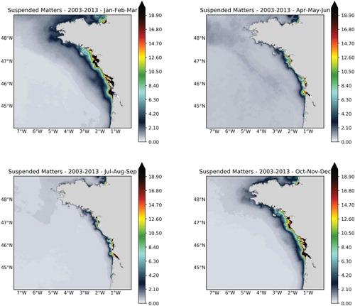
During the MODYCOT 99-3 experiment (Puillat et al. 2004), the Gironde river plume reached the offshore area of the Loire estuary and a lens of 100–150 $\mathrm{km}$ diameter is formed. The Loire and Gironde river plumes form northward currents parallel to the coast which have been observed using surface drifting buoy trajectories (Castaing 1984, Puillat et al. 2004). The Loire and Gironde river plumes extension is maximal in winter with a peak in January ($3\times {10}^4{\mathrm{km}}^2$) and it is minimal in summer with a low extension in July ($4\times {10}^3{\mathrm{km}}^2$) (figure 1) (Lazure and Jegou 1998). The inflow speed is $u_e=Q/(hL)$, where h is the maximum estuarine depth, Q the river discharge and L the width at the estuary mouth. The maximum and minimum inflow speeds occur respectively in winter and summer, with a maximum in January of about $2\mathrm{cm}{\mathrm{s}}^{-1}$ for the Gironde (a mouth width of $\sim 10\mathrm{km}$ and depth of $\sim 10\mathrm{m}$) and $\sim 1\mathrm{cm}{\mathrm{s}}^{-1}$ for the Loire river (a depth of $\sim 10\mathrm{m}$ and a mouth width of $\sim 20\mathrm{km}$) and a minimum in August of $\sim 0.5\mathrm{cm}{\mathrm{s}}^{-1}$ for the Gironde river and $\sim 0.25\mathrm{cm}{\mathrm{s}}^{-1}$ in Loire river (Costoya et al. 2017). We note that the inflow speed is the residual (tides filtered) inflow from the estuary to the open ocean. Phytoplankton and zooplankton seasonal cycles are also sensitive to the river plume dynamics, which is subject to mixing and stratification modifying the photosynthetic available radiations (Botas et al. 1990, Lavín et al. 2006).

River plumes can be affected by various, geostrophic or ageostrophic, instabilities, due to the velocity and density anomalies that they create in the coastal ocean. Ambient stratification or bottom topography can also influence these instabilities. In the bulge and frontal regions, the main instabilities are baroclinic, barotropic and Kelvin–Helmholtz instabilities.

Baroclinic instabilities can occur for wide plumes (Hetland 2017). Baroclinic instabilities of the Gaspe current (the freshwater current originating from the St Lawrence estuary) have been observed in SST images and have been modelled numerically at 2–3 km resolution (Sheng 2001), but few observations of barotropic instabilities are available. For tidally forced plumes, Kelvin–Helmholtz billows can result from vertical shear instability of horizontal currents at the bottom of the plume, in the near-field region. This instability also increases the mixing of freshwater with ambient saline water (MacDonald and Geyer 2004, Kilcher and Nash 2010).

The instabilities affecting narrow river plumes (with estuary width limited to a few kilometers) under external forcing have not yet been studied with a very high-resolution model. With a two-layer model, de Kok (1997) shows that northeasterly and easterly winds favour the stratification onset, and baroclinic instability in a Rhine river plume settings. This instability creates salinity front meanders which considerably reduce the trapped coastal water. Winds or tides tend to inhibit instabilities through mixing. Instabilities are strongest in summer and mixing overcomes instabilities in other seasons (Hetland 2017).

In the present work, a submesoscale resolving model is used to perform idealised numerical simulations of a river plume (the Gironde). In particular, we will address the following questions:

• what is the 3D structure of this plume, considering the bulge and the coastal current?

• what is the effect of different forcings (wind, tidal, mean flow…) on this structure?

• which types of instabilities, both geostrophic and ageostrophic can affect this plume and under which conditions?

• what are the consequences of the instabilities on the 3D mesoscale structure of the plume, in particular via the vertical mixing induced by the submesoscale features, and via the energy transfer that they achieve?

The paper will thus be organised as follows: the model configuration, simulations and methods will be described in section 2, the 3D structure of the plume in section 3.1, the instabilities affecting it in section 3.2 and the impact of submesoscale effects on the plume structure in section 3.3. The main results will be discussed in section 4 and conclusions will be provided.

2. Materials and methods

2.1. Model configuration

The simulations are performed using the Coastal and Regional COmmunity CROCO. CROCO and CROCO TOOLS are provided by https://www.croco-ocean.org (Shchepetkin and McWilliams 2005, Debreu et al. 2012). CROCO (based on ROMS) is a split-explicit, free-surface, hydrostatic, primitive equation ocean model. The model uses sigma coordinates in the vertical; orthogonal curvilinear coordinates are used in the horizontal; the variables are discretised on an Arakawa C-Grid. The horizontal resolution is 200 m; 128 σ-layers discretise the flow vertically; these layers are stretched at the surface and at the bottom with ${\theta }_s=5$, ${\theta }_b=0.4$ and $h_{min}=10\mathrm{m}$. The model time step is $30\mathrm{s}$ with model outputs every 2 h.

The horizontal advection of momentum and tracers is performed with the Zico extension fifth order WENO scheme (a weighted ENO with improvements of the weights formula) (Rathan and Raju 2016). It has the advantage of being little dissipative and of not imposing a CFL (Courant-Friedrichs-Lewy) constraint. The vertical advection is a parabolic conservative scheme for both momentum and tracers. The model implicit vertical mixing is configured using the $k-\omega$ turbulent closure scheme with a Kantha Clayson stability function (Kantha and Clayson 1994, Umlauf and Burchard 2005, Warner et al. 2005). The background vertical diffusivities (for both momentum and tracers) are $K{v}_b=5\times {10}^{-6}{\mathrm{m}}^2{\mathrm{s}}^{-1}$ and $K{t}_b=5\times {10}^{-6}{\mathrm{m}}^2{\mathrm{s}}^{-1}$. A Smagorinsky-like viscosity have been used for lock-exchange problem which takes place when two reservoirs of different densities interact with each other in a horizontal closed domain (Gröbelbauer et al. 1993, Lowe et al. 2005). The quadratic Von-Karman law (logarithmic law) is used for bottom friction with a bottom roughness $z_0=5\mathrm{mm}$.

The domain extent is [142 km, 445 km, 100 m] in the x, y, z directions respectively with a bathymetry varying zonally (no meridional variations) (figure 2).

Figure 2. Bathymetry of the idealised numerical model configuration. (Colour online)

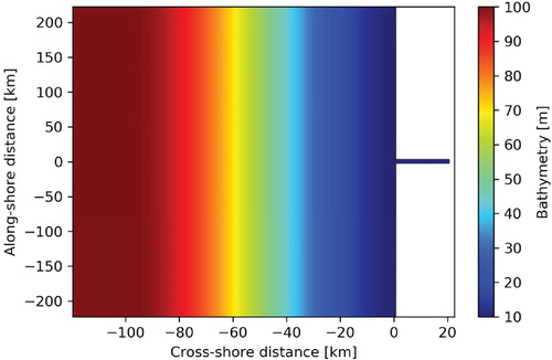
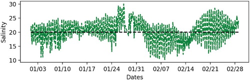
The estuary is located in the middle of the domain with a 20 km length, 6 km width and a uniform depth of 10 m. The freshwater discharge is prescribed in the eastern, most, part of the estuary; it is distributed over 31 grid points and ramped over 2 days with a hyperbolic tangent tendency. The freshwater sources temperature and salinity are 13${}^{\circ }$C and 20 psu, respectively. The freshwater source salinity is chosen as an average from the MAGEST in situ observing network time series (at 1 m depth) during the January–February 2019 period as shown in figure 3. The Le Verdon station was considered here; its location is shown in figure 1.

Figure 3. Le Verdon MAGEST station time series of salinity at $\sim 1\mathrm{m}$ depth during January and February 2019. The black dashed line shows the 20 psu salinity value used for idealised simulations. (Colour online)

The initial conditions are rest (no current) with a homogenous ocean ($T_0={13}^{\circ }$C and $S_0=35\mathrm{psu}$). The background temperature and salinity values are based on BOBYCLIM, an in situ climatology in the Bay of Biscay (Vandermeirsch et al. 2010). Following previous studies (Vic et al. 2014, Palma and Matano 2017), we choose similar values for background and freshwater temperatures. A simulation using a different freshwater temperature (9${}^{\circ }$C instead of 13${}^{\circ }$C) has been compared to the reference configuration. We show that the change in temperature has a small effect on the circulation and the buoyancy in the river plume without changing its global shape or structure. For example, after 12 simulated days, we obtain small differences in sea surface height ($\sim 0.7\mathrm{cm}$), in the vertically averaged u and v momentum ($\sim 4\mathrm{cm}{\mathrm{s}}^{-1}$) and in the vertically averaged density ($\sim 0.6\mathrm{kg}{\mathrm{m}}^{-3}$). Therefore, we decide to consider the 13${}^{\circ }$C freshwater temperature similar to the background values. In the case of non-tidal simulation, the Orlanski-type (Orlanski 1976) open boundaries conditions for both momentum (2D and 3D) and tracers is used at the western, southern and northern part of the domain; a sponge layer of $30\mathrm{km}$ is added with a cosine profile viscosity (values ranging from 0 (inner boundary) to $13{\mathrm{m}}^2{\mathrm{s}}^{-1}$ (outer boundary)) to avoid reflections and to dissipate any noise generated at the boundaries. In the tidal case, we used Chapman open boundary conditions for the surface elevation (Chapman 1985), and Flather open boundary conditions for the barotropic velocity components combination (Marchesiello et al. 2001). For the 3D tracers and momentum, an Orlanski open boundary condition is used. A sponge layer was also used. This idealised configuration is based on the Gironde river plume dynamics for different parameters (i.e. salinity gradients, estuary width, river discharge, bathymetry slope) but we decided not to consider supplementary constraints such as the coastal shape (including existing small islands) or other existing rivers (as the Loire river plume further North in the Bay of Biscay) to avoid complex interactions. This choice was dedicated to optimise numerical framework to understand instability and mixing dynamics in the river plume.

2.2. Model experiments

In this part, a description of the sensitivity experiments simulated in this study is provided. The duration of all the numerical simulations presented in this study is 16 days. The simulation length is based on two criteria: first, it has been defined as the typical time range necessary, in idealised condition, to reach a balanced regime in the river plume and to have at least one week for analyses; the second is related to the observed high river discharge in winter. As shown in figure 4, the simulated river discharge is close to winter monthly averages values.

Figure 4. The Gironde estuary is fed by the Garonne and Dordogne rivers. The discharges for these two rivers are obtained from hydrological stations and retrieved through the French national service “Banque Hydro” (https://www.hydro.eaufrance.fr). They are added together to estimate the Gironde discharge. Blue dots show the monthly discharge mean. For each month, the standard deviation of the river discharge is represented by a vertical bar. The red dashed line shows the $1550{\mathrm{m}}^3{\mathrm{s}}^{-1}$ discharge value used in idealised simulations. (Colour online)

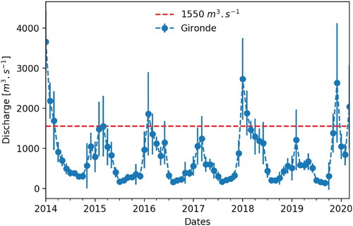
The reference experiment has a river discharge of $1550{\mathrm{m}}^3{\mathrm{s}}^{-1}$ and no external forcing. The discharge value defined here is based on monthly-averaged observations from hydrological stations, provided by the French national service “Banque Hydro” (https://www.hydro.eaufrance.fr). These discharge values correspond to estuarine flood periods. Sensitivity to a high discharge value of $\mathrm{10,000}{\mathrm{m}}^3{\mathrm{s}}^{-1}$ has been studied without external forcings to evaluate the model response to extreme flux conditions. Such a high discharge is not reached in the Bay of Biscay but has been studied here to explore the Gironde river plume in the case of an extreme (unrealistic) flood. This extreme river discharge helps to understand the dynamics for plumes comparable to the Congo or the Mississippi river (Vic et al. 2014, Hetland 2017). Sensitivity to tides has been analysed using the reference discharge and M2 tide component with an amplitude of 1.5 m. Model outputs (M2 tide cofiguration) have been detided using a Fast Fourier Transform (FFT) as in Walters and Heston (1982). To investigate the impact of the southwesterly wind regime, no wind is applied during the first 8 simulation days then the wind stress is ramped over 4 days (with a tanh tendency) up to ${\tau }_{max}=0.02\mathrm{N}{\mathrm{m}}^{-2}$. Table 1 summarises the configurations used in the present study.

Table 1. List of simulations and their specific forcings.

Experiments	River forcing	External forcings
Reference	Discharge ($1550{\mathrm{m}}^3{\mathrm{s}}^{-1}$)	–
High Discharge	Discharge ($\mathrm{10,000}{\mathrm{m}}^3{\mathrm{s}}^{-1}$)	–
Tide	Discharge ($1550{\mathrm{m}}^3{\mathrm{s}}^{-1}$)	M2 Tide (1.5 m amplitude)
Wind	Discharge ($1550{\mathrm{m}}^3{\mathrm{s}}^{-1}$)	SW Wind (${\tau }_{max}=0.02\mathrm{N}{\mathrm{m}}^{-2}$)

2.3. Methods

2.3.1. Diagnostics for river plume instabilities

The instability of river plumes leading to the generation of eddy kinetic energy is analysed using the transfer of kinetic and potential energy from the mean to the submesoscale turbulent flows. A scale decomposition is performed on the velocity and buoyancy fields. In this decomposition, the mean flow represents the large scales and perturbations represent the meso-scales and submeso-scales. The decomposition on the velocity and buoyancy fields is expressed as $\mathit{u}=\overline{\mathit{u}}+{\mathit{u}}^{\prime }$ and $b=\overline{b}+b^{\prime }$. Overbar and prime denote temporal mean over one day as follows $\overline{\bullet }=(1/T){\int }_{t-T/2}^{t+T/2}\bullet \mathrm{d}t$ (mean flow) and deviations relative to this mean (perturbations), respectively. The horizontal (HRS) and vertical (VRS) shear stresses and the vertical buoyancy flux (VBF) (instantaneous values) are expressed as in Gula et al. (2016) and Capuano et al. (2018) as (1) $\begin{array}{rl}\mathrm{HRS}& =-u^{\mathrm{\prime }2}{\mathrm{\partial }}_x\overline{u}-u^{\mathrm{\prime }}{v}^{\mathrm{\prime }}[{\mathrm{\partial }}_y\overline{u}+{\mathrm{\partial }}_x\overline{v}]-v^{\mathrm{\prime }2}{\mathrm{\partial }}_y\overline{v},\end{array}$(1) (2) $\begin{array}{rl}\mathrm{VRS}& =-u^{\mathrm{\prime }}{w}^{\mathrm{\prime }}{\mathrm{\partial }}_z\overline{u}-v^{\mathrm{\prime }}{\mathrm{\partial }}_z\overline{v},\end{array}$(2) (3) $\begin{array}{rl}\mathrm{VBF}& =w^{\mathrm{\prime }}{b}^{\mathrm{\prime }}.\end{array}$(3) Barotropic instability is characterised by a positive HRS (transfer from MKE (mean kinetic energy) to EKE (eddy kinetic energy)). Baroclinic instability is related to a positive vertical buoyancy flux (VBF). Mixed barotropic and baroclinic instabilities occur when VBF and HRS are positive at the same location. Kelvin–Helmholtz instability is represented as a positive VRS. Negative values of VBF, VRS, HRS represent a contribution to the mean flow (Kang 2015, Evans Contreras et al. 2019).

Submesoscale processes and their contribution to instabilities can be related to changes in the Ertel potential vorticity (Q) (Ertel 1942, Schubert et al. 2004) and in stratification due to external forcings (winds, tides, eddies). The Ertel potential vorticity can be expressed in isopycnal coordinates as (Morel and McWilliams 2001) (4) $Q=\frac{f+{\zeta }_{\rho }}{h_{\rho }},$(4) where ${\zeta }_{\rho }=({\mathrm{\partial }}_{x}v-{\mathrm{\partial }}_{y}u{)}_{\rho }$ is the relative vorticity computed in isopycnal coordinates, $h_{\rho }$ is the isopycnal thickness and f is the Coriolis parameter.

The rotation, stratification and vertical shear are important to understand the river plume dynamics (Nash et al. 2009, Pan and Jay 2009). Therefore to understand the nature of the regime (geostrophic or ageostrophic) and to understand the importance of shear mixing in river plumes, we will analyse the Richardson Number and the local Rossby Number expressed as (5) $R_o=\frac{{\mathrm{\partial }}_{x}v-{\mathrm{\partial }}_{y}u}{f},R_i=\frac{N^2}{S^2},$(5) where $N^2=-(g/{\rho }_0){\mathrm{\partial }}_z\rho$ is the Brunt-Vaisala frequency and $S^2=({\mathrm{\partial }}_{z}u{)}^2+({\mathrm{\partial }}_{z}v{)}^2$ is the vertical shear in which u and v are the instantaneous along-shore and cross-shore velocities, respectively.

When $R_i$ and $R_o$ are $\mathrm{O}(1)$ submesoscale processes prevail (Thomas et al. 2008, McWilliams 2016). According to the criteria of Hoskins (1974), negative fQ and $R_i<1$ indicate the existence of symmetric instabilities (see also Morel and McWilliams 2001, Thomas et al. 2013). We calculate the cross-shore gradient ${\mathrm{\partial }}_{x}Q$. We identify where its sign changes across and along isopycnals. This indicates baroclinic and barotropic instabilities (Charney–Stern criterion).

2.3.2. Diagnostics for river plume vertical mixing

The last diagnostics for this paper is to analyse changes in stratification in a given volume driven by two main mechanisms: frontogenesis and changes in potential vorticity (Marshall and Nurser 1992, Marshall et al. 2001, Lapeyre et al. 2006, Thomas and Ferrari 2008). In our case, we consider the volume, variable in time, delimited by the outcropping at the surface to the river plume base (isopycnals $1024\mathrm{kg}{\mathrm{m}}^{-3}$ for Reference,Tide and SW wind simulations and $1022\mathrm{kg}{\mathrm{m}}^{-3}$ for High discharge simulation). We write the mean stratification over the considered volume (6) $f\mathrm{\Delta }\overline{N^2}=\mathrm{FRONT}+\mathrm{\Delta }q.$(6) Here we express the frontogenesis term (FRONT) as the temporal cumulative sum of ${\int }_{V(t)}{\mathrm{\partial }}_t(\zeta b)\mathrm{d}V$ over previous time steps (here 2 h) where ζ is the relative vorticity and $b=-g\rho /{\rho }_0$ is the buoyancy. Where ${\rho }_0$ is the mean density in the domain. The potential vorticity is expressed as (7) $q={\int }_V{\mathit{\omega }}_a\mathbf{\cdot }\mathbf{\nabla }b\mathrm{d}V,$(7) where ${\mathit{\omega }}_a=f\mathit{k}+\mathbf{\nabla }\times \mathit{u}$.

Following Marshall and Nurser (1992), we write the equation of conservation of Ertel potential vorticity as (8) ${\mathrm{\partial }}_{t}q+\mathbf{\nabla }\mathbf{\cdot }\mathit{J}=0$(8) which leads to (9) ${\mathrm{\partial }}_{t}q=-\mathit{u}\mathbf{\cdot }\mathbf{\nabla }q+(\mathbf{\nabla }\times \mathit{F})\mathbf{\cdot }\mathbf{\nabla }b+(f\mathit{k}+\mathbf{\nabla }\times \mathit{u})\mathbf{\cdot }\mathbf{\nabla }D.$(9) The terms on the right-hand side of this equation represent advection (first term), torque or friction (second term) and buoyancy fluxes (third term). The second and third terms are related to vertical mixing of mass or momentum that we can write as (10) $F=\mathbf{\nabla }\mathbf{\cdot }(K_m{\mathrm{\partial }}_z{\mathit{u}}_h)=F_v.$(10) where the subscript h denotes the horizontal components. In addition, F is the body force in Navier-Stokes, which can be related to vertical mixing of momentum ($F_v$) (we neglect here lateral mixing ($F_l$), it is implicit in the advection scheme of our model). In the CROCO model, surface and bottom forcings in vertical mixing of momentum are parametrised by wind stress and bottom stress. The third term is related to vertical mixing of tracers (remember that ocean and river temperatures are the same). We write (11) $D={\mathrm{\partial }}_z(K_b{\mathrm{\partial }}_{z}b),$(11) where D is the source term in the mass conservation equation (no explicit horizontal diffusivity is considered here), which here is represented by the vertical mixing of buoyancy. At the surface, vertical mixing of mass can be associated to river input, heat exchange, and evaporation and precipitation. Thus, one can express the fluctuations in potential vorticity as resulting from friction, diabatic and advection processes (12) $\frac{\mathrm{\partial }q}{\mathrm{\partial }t}=\mathrm{ADV}+\mathrm{FRIC}+\mathrm{DIAB}+\mathrm{Pres}.$(12) The last term (Pres) represents the curl of pressure gradient (zero by definition). The last equation is analysed in a volume that varies in time (13) ${\mathrm{\partial }}_t{\int }_{V(t)}q\mathrm{d}V={\int }_{V(t)}(\mathrm{ADV}+\mathrm{FRIC}+\mathrm{DIAB})\mathrm{d}V+\mathrm{BVP}.$(13) The last term represents the PV advection along the bounding isopycnals here the surface and the river plume base. The ADV (advective mixing), FRIC (frictionless mixing), DIAB (diabatic mixing), Pres (Pressure) and BVP (boundary value problem) are detailed in Appendix and are discussed in Callendar et al. (2011).

3. Results

3.1. River plume 3D structure and dynamics

In this part, the interaction of the river freshwater with the open ocean and its sensitivity to different forcing are analysed by means of 3D hydrological and dynamical structures.

3.1.1. Reference configuration

The river plume is divided into two regions: the anticyclonic gyre (bulge) and the coastal current (figure 5). The river plume evolves in three steps as shown in figure 5.

Figure 5. Sea Surface Salinity at three different time steps – Reference Configuration. The black dashed line represents zonal vertical sections shown hereafter. The bold black rectangle represents the bulge region. The bold dashed rectangle defines the coastal current. (Colour online)

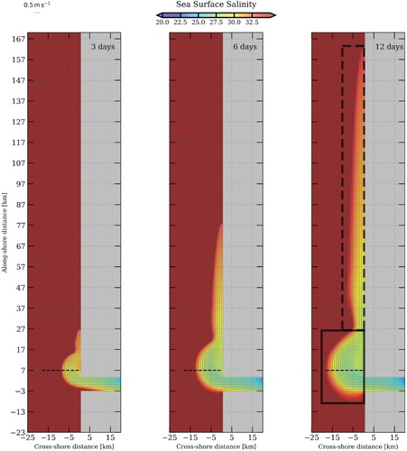
During the first stage, the bulge expands, trapping water exiting from the estuary. In this case, the salinity value increases from 20 to 30 psu, from the river to the bulge. This indicates mixing of the freshwater with the seawater (which has salinity of 35 psu); note also that some seawater enters the estuary, on its southern side, during this stage. This shows that the outflow at the river estuary undergoes some adjustment and is not yet steady. The second stage lasts from days 3 to 10 approximately. Then, the riverine freshwater feeds the bulge, where the salinity decreases from 30 to 25 psu. Thus the mixed water concentrates at the edge of the bulge, forming a salinity front. In this case, seawater is not detected into the estuary. The bulge itself starts to feed the coastal current which progresses northward along the coast as a coastal surface current of freshwater. In the third stage (after day 10), the coastal current is well established for more than 100 km northward (though its nose continues to head northward) and instabilities can develop along it. The coastal current width reaches half of the bulge. The surface salinity map shows a complex pattern in the bulge with strong gradients near the coast. This is due to the recirculation of the riverine water at this location. This pattern will appear even more clearly in the surface relative vorticity map. For the study of the plume structure, we will consider that the flow state at day 12 is a quasi-final situation with both a bulge and an established coastal current.

At this time, the bulge width and depth reach 20 km and 5 m (see the vertical section of density at alongshore distance 7 km on figure 6(a)).

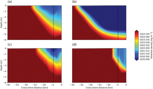
Figure 6. Vertical sections of Potential density (day 12): (a) Reference, (b) High Discharge, (c) Tide, (d) SW wind. The black dashed line represents the vertical profiles (density and $N^2$) shown hereafter. (Colour online)

The river plume base is located at $\sim 4\mathrm{m}$ depth (with a density gradient between 3 and $5\mathrm{m}$ depth) or near the isopycnal $1024\mathrm{kg}{\mathrm{m}}^{-3}$. A measure of the freshwater thickness in the bulge or the coastal current is defined by Hetland (2005) as (14) $h_f={\int }_{-H}^0(1-\frac{S}{S_0})\mathrm{d}z,$(14) i.e. via an integral from the local bottom to the surface of the ocean; $S_0$ is the background salinity (here 35 psu) and S is the local plume salinity. The value thus obtained for the freshwater thickness (2 m) is well correlated with the potential density profile which shows a maximal gradient between 3 and 5 m depths (figure 7).

Figure 7. Brunt–Vaisala (left) and potential density (right) vertical profiles (12 day). (Colour online)

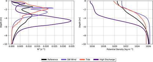
The buoyancy vertical gradient (Brunt–Vaisala frequency) has a peak at 3.5 m depth which is equivalent to the river plume base depth ($\sim 4\mathrm{m}$). A secondary peak of the buoyancy vertical gradient at 1.5 m depth is related to the surface recirculation of the freshwater in the bulge.

Figure 8(a) is a horizontal map of the relative vorticity at day 12 for the end state of the plume.

Figure 8. Surface scaled relative vorticity (day 12): (a) Reference, (b) High Discharge, (c) Tide, (d) SW wind. (Colour online)

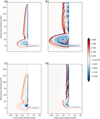
The circulation in the bulge is anticyclonic except at two locations: (a) in its core where a small filament of positive vorticity can be seen due to freshwater recirculation, and (b) in the frontal region, where a narrow strip of positive vorticity lies between the ambient and the fresh water masses. In the coastal current, positive relative vorticity is also found in the frontal region, while strong negative vorticity ($\zeta /f<-1$) is located near the coast due to the frictional effect there (thus forming a strong shear layer). The flow is clearly ageostrophic ($R_o\sim \mathrm{O}(1)$) at fronts and where strong curvature occurs, i.e. around the bulge, between the bulge and the coastal current, and at the northern nose of the coastal current. Vertically, the relative vorticity distribution (at alongshore position 7 km) is as follows. Near the surface (top 2 m) and near the estuary mouth (5 km from the coast), the local Rossby Number $R_o\sim \mathrm{O}(1)$ (figure 9(a)).

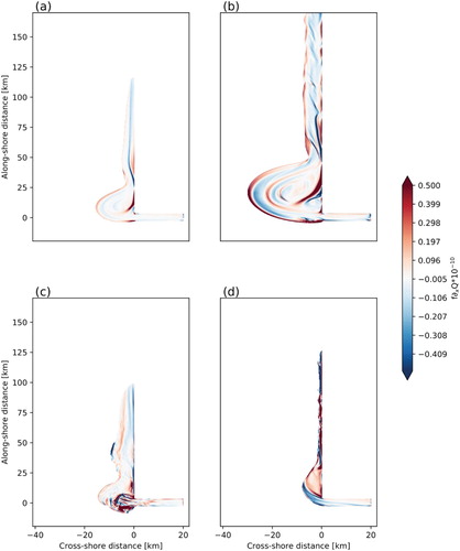
Figure 9. Vertical sections of scaled relative vorticity (day 12): (a) Reference, (b) High Discharge, (c) Tide, (d) SW wind. (Colour online)

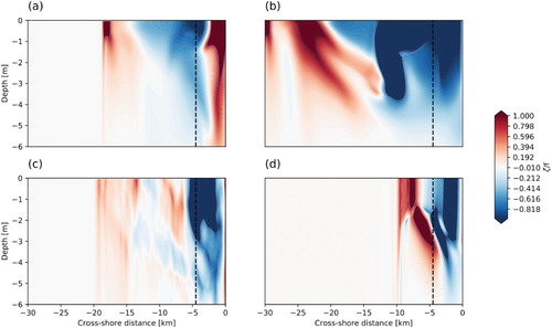
High Rossby numbers ($R_o\sim \mathrm{O}(1)$) are also found in the frontal region, in a thin layer of 1 m depth and roughly 1 km width. In the other parts of the bulge, $R_o<1$. This shows coexistence of geostrophic and ageostrophic motions in the bulge. The latter is in good agreement with the total kinetic energy spectrum as it is characterised by a $k^{-2}$ slope at the river plume base and by a slope between $k^{-3}$ and $k^{-4}$ at the surface (figure 10).

Figure 10. KE density spectrum at the surface (left) and at the river plume base (right). (Colour online)

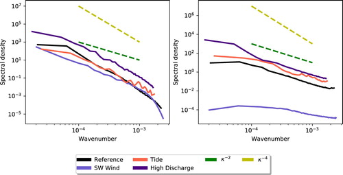
Thus, the dynamics is essentially driven by balanced processes near the surface, while frontal and ageostrophic processes dominate the evolution of the plume base.

3.1.2. Sensitivity experiments

External forcings have a noticeable impact on the horizontal and vertical shape and structure of the river plume. In the case of high discharge, the bulge develops quickly (figure 11): after 2 days, its width already reaches 15 km (the final size of the bulge in the reference configuration) and it grows to 30 km after 12 days.

Figure 11. Sea surface salinity at three different time steps – high discharge configuration. The black dashed line represents zonal vertical sections shown hereafter. (Colour online)

Under these conditions seawater is not able to penetrate into the estuary because the strong outward flux prevents it. The coastal current then extends to more than 160 km northward after 12 days. Its width represents half of that of the bulge. Salinity values are now significantly higher than 20 psu only in the coastal current, which faces the open sea, and at the centre of the bulge which contains the riverine water that has outflowed first, and has slightly mixed with seawater. The strong outflow velocities constrain water mixing to a occur in a thin frontal region, highly sheared. In the final stage (day 12), the vertical section of density (figure 6(b)) also shows a high gradient concentrated both on the side and below the bulge. Correspondingly, a higher density stratification is now observed at a depth of 5 m or near the $1022\mathrm{kg}{\mathrm{m}}^{-3}$ isopycnal, with a freshwater thickness of 3 m (figure 7). Again, a near surface peak in vertical buoyancy gradient is related to the surface freshwater recirculation (in the upper meter).

In terms of relative vorticity, intense circulation occurs in the bulge with spiral strips of positive vorticity. This strip detaches from the frictional layer at the coast and wraps into the growing bulge. A thin layer of positive vorticity can again be seen at the edge of the bulge and of the coastal current (in the frontal region with the open sea, see figure 8(b)). Ageostrophic motions ($R_o\sim \mathrm{O}(1)$) are present at the edges and within the core of the bulge in the top 5 m. The more intense circulation here leads to larger horizontal and vertical velocity shears; filamentary instability of the coastal current front and shear instability at the coast, forming a row of small vortices, result from these velocity shears (figure 8(b)).

When forced by SW winds, the river plume grows slowly and weakly with regards to the bulge extension (figure 12).

Figure 12. Sea surface salinity at three different time steps – SW Wind Configuration. The black dashed line represents zonal vertical sections shown hereafter. (Colour online)

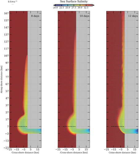
Indeed, the offshore edge of the bulge reaches barely 5 km by the end of the simulation when the wind intensity is at its highest. The maximum wind intensity reached in our study is ${\tau }_{max}=0.02\mathrm{N}{\mathrm{m}}^{-2}$. The wind direction chosen here corresponds to a winter situation (where the ocean is homogeneous) as shown in Le Boyer et al. (2013) (their figure 5). The bulge slowly grows during 8 days before the onset of the wind. After this period, the southeastward Ekman transport promoted by SW winds (winds blowing toward the coast, not alongshore, when Ekman transport is intensified) prevents the bulge from growing more, acting against the river outflow, and pressing the bulge close to the coast. Therefore, this wind direction (SW winds) favours a more intense plume development toward the north and lower salinity values resulting from the plume confinement toward the coast. The coastal current is very thin (less than 3 km wide), patchy and its water is strongly diluted with seawater (salinity values reach 32 psu at kilometre 150 in alongshore distance). In the vertical section of density (at kilometre 7 in alongshore distance), an outcropping can be seen near the coast, as freshwater is pushed to the coast by Ekman transport (figure 6(d)). In terms of relative vorticity, the external frontal region is perturbed by short waves (figure 8(d)) so that relative vorticity (or Rossby number) significantly varies around the bulge rim. The coastal current has a jet-like shape (being narrow, it is strongly sheared on both sides), and the features of instability (filaments and meanders) generate local curvature and ageostrophic motions ($R_o\sim \mathrm{O}(1)$). Frontal activity (strong ageostrophic motions) can be observed through the river plume vertical structure corresponding to strong local Rossby number on both sides of the jet. Here the front is $\sim 1\mathrm{km}$ wide and frontal activity is constrained by the effective resolution of the model.

When tide acts on the plume, the bulge and coastal current grow through the 12 days of simulation and the bulge finally reaches a width of 15 km. Nevertheless, their spatial structure is complex. Firstly, seawater penetrates into the estuary (see days 3 and 6 in figure 13) when shoreward motion is favoured by the tidal flow.

Figure 13. Sea surface salinity at three different time steps – Tide Configuration. The black dashed line represents zonal vertical sections shown hereafter. (Colour online)

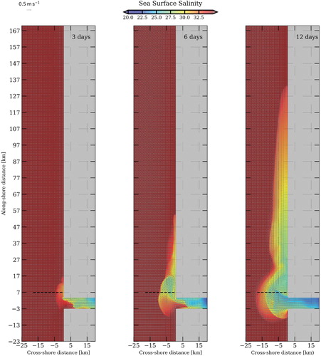
Secondly, several salinity fronts exist both in the bulge and in the coastal current. They are due to the local concentration of salt by the tidal oscillation (see figure 13). Furthermore, the current oscillation also results in local concentrations of velocity shear, hence of mixing. This results in a succession of increasingly mixed areas seaward, in the whole plume. The vertical density structure of the river plume also shows these oscillations (figure 6(c)). Saltier water is located between the core of the bulge and the coast, again due to the fact that the bulge is fed by bursts of freshwater. In the river plume, the vertical density gradient lies between 2 and 4 m depth and the freshwater thickness is 2 m (figure 7). Figure 8(c) confirms that several fronts exist in both the bulge and the coastal current; these are locations of strong positive relative vorticity ($R_o\sim \mathrm{O}(1)$). These positive vorticity strips are linked to previous tidal pulsations. Highly negative relative vorticity is found at the coast (again due to the velocity shear there) and in the bulge, north of the estuary, close to the coast (again where the current is strongly sheared). The vertical structure of the Rossby number shows different strong scaled vorticity ($R_o\sim \mathrm{O}(1)$) in the near field (5 km from the coast and top 3 m) and weak scaled vorticity ($R_o<1$) in the far field, except along vertical strips, corresponding to the fronts previously mentioned (figure 9(c)).

3.2. River plume instability analysis

3.2.1. Reference configuration

The isopycnic Charney-Stern criterion (CSC) was calculated with the cross-shore Ertel potential vorticity gradient (${\mathrm{\partial }}_{x}Q$) at the base of the river plume (remember that the Rossby number is large at the edge of the plume). This gradient changes sign both in the bulge and in the coastal current (figure 14(a)); in the bulge, sign reversals are found both at the external front and near the coast, north of the estuary.

Figure 14. $f{\mathrm{\partial }}_{x}Q$ at the river plume base (day 12) for (a) Reference, (b) High Discharge, (c) Tide, (d) SW wind. (Colour online)

Again, this corresponds to the strong velocity shears previously mentioned. In the coastal current, the sign reversal occurs twice (between the frictional layer at the coast and the jet axis, and between the jet axis and the external front).

Figure 15(a) shows a vertical section of CSC along the zonal section north of the estuary. In the bulge, ${\mathrm{\partial }}_{x}Q$ changes sign both along and across isopycnals.

Figure 15. Vertical section $f{\mathrm{\partial }}_{x}Q$ (day 12) for (a) Reference, (b) High Discharge, (c) Tide, (d) SW wind. (Colour online)

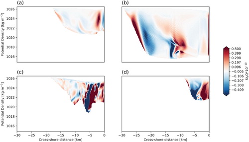
In the near field (5 km from the coast), ${\mathrm{\partial }}_{x}Q$ values are large and change sign mostly along isopycnals. At the bulge periphery, the distribution of ${\mathrm{\partial }}_{x}Q$ is more filamentary and is weaker with positive and negative values. These elements suggest that barotropic instability is more likely to develop, in particular near the coast. Baroclinic instability is not ruled out but may be weaker.

To investigate the possibility of non-geostrophic instability (symmetric instability or Kelvin–Helmholtz instability), we also examine the distributions of fQ and of the Richardson number $R_i$ (figures 16(a) and 17(a)).

Figure 16. fQ at the river plume base (day 12) for (a) Reference, (b) High discharge, (c) Tide, (d) SW wind. (Colour online)

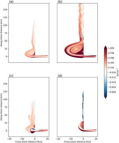
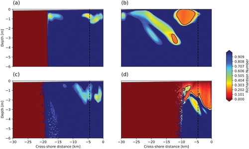
Figure 17. Richardson number at the river plume base (day 12) for (a) Reference, (b) High discharge, (c) Tide, (d) SW wind. (Colour online)

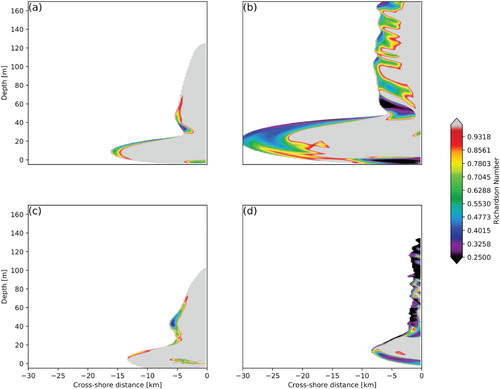
At the river plume base fQ is positive almost everywhere in the river plume except in a narrow region in the coastal current where weak negative values can be observed. At the river plume base, the Richardson number values are $R_i\sim \mathrm{O}(1)$ almost everywhere except at the northern edge of the bulge and at the junction between the bulge and the coastal current ($R_i$ higher than 0.25 and lower than 1) (figure 17(a)). This suggests that symmetric instability and vertical shear instabilities are not strong in this case.

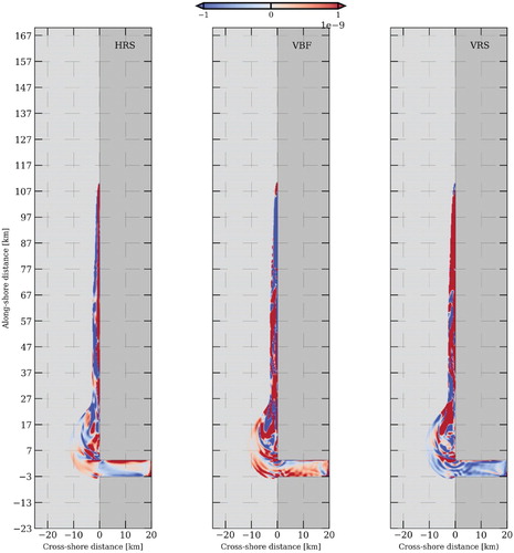
Now, we present vertically integrated values from the plume base to the surface of the energy transfers HRS, VRS and VBF when the plume is developed (day 10). We will show that these values are weaker in the reference configuration than in the sensitivity experiments. This is due to the fact that the plume gains energy when forcing is added. The energy of this mean flow can then feed the perturbations.

In this reference configuration, weak positive values for the vertically integrated HRS, VBF and VRS are found in the river plume (figure 18).

Figure 18. Integrated (from river plume base to surface – day 10) HRS (left),VBF (middle) and VRS (right) for the reference configuration. (Colour online)

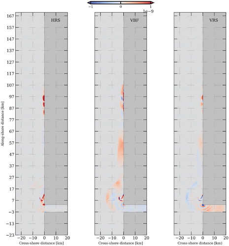
Higher HRS and VRS values can be observed in the bulge at the transition near the coast and the estuary. This is due to high and baroclinic fluid acceleration and the bulge recirculation. Positive HRS values can be observed at the southern and northern edges of the bulge, in the recirculation region of this latter and in the coastal current. Both positive and negative values of HRS are concentrated at the edges of freshwater recirculation in the bulge. VBF is concentrated in the periphery of the bulge and in the coastal current. VRS is very small. These results are in agreement with the stability criteria previously examined, showing that barotropic instability is dominant (in particular at the estuary), and baroclinic instability may occur rather at the rim of the bulge but they (instabilities) do not seem to grow significantly.

3.2.2. Sensitivity experiments

Firstly, we examine the case of a high rate of discharge. At the river plume base, narrow and intense filaments of negative and positive ${\mathrm{\partial }}_{x}Q$ (cross-shore gradient of isopycnic Ertel potential vorticity) are found all across the bulge and the coastal current (figure 14(b)). The vertical section of this quantity shows that this gradient changes sign both across and along isopycnals inside the bulge and at its edges (figure 15(b)).

At the river plume base, fQ is negative in the coastal current near the coast (figure 16(b)), indicating symmetric instability there. At the western edge of the coastal current, and near its junction with the bulge, the Richardson number ranges from 0.25 to 1, likely related to Kelvin–Helmholtz instability (figure 17(b)). At the rim of the bulge, values of the Richardson number also range in $0.25<R_i<1$. The vertical section north of the estuary shows negative values of fQ near the surface of the bulge (figure 19(b)), well correlated with patches of $R_i<0.25$; patches of low $R_i$ are also found at the base of the bulge (at 3 m depth; see figure 20(b)).

Figure 19. Vertical sections (isopycnes) fQ (day 12) for (a) Reference, (b) High Discharge, (c) Tide, (d) SW wind. (Colour online)

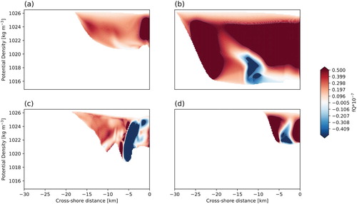
Figure 20. Vertical section Richardson Number (day 12) for (a) Reference, (b) High Discharge, (c) Tide, (d) SW wind. The black solid contour indicates the critical Richardson number $R{i}_c=0.25$. (Colour online)

For a high rate of discharge, strong positive HRS, VBF and VRS values are found in the core of the bulge, at its western and/or southwestern edges and in the coastal current (figure 21).

Figure 21. Integrated (from river plume base to surface – day 10) HRS (left),VBF (middle) and VRS (right) for the high discharge configuration. (Colour online)

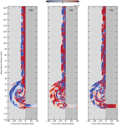
In this latter, HRS is strong near the coast, while VBF and VRS are intense in the northern and external region. In the northern part of the bulge, near the coastal current, negative HRS, VBF and VRS values can be observed. Therefore, barotropic, baroclinic and Kelvin–Helmholtz instabilities develop in the bulge and in the coastal current. This is confirmed in particular by the map of scaled relative vorticity at day 12 showing filaments southwest of the bulge and at the edge of the coastal current and small vortices along the coast, in the coastal current. In this case, vertical shear, horizontal shear (barotropic), symmetric and baroclinic instabilities exist in different regions of the river plume.

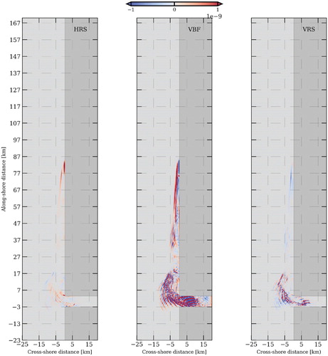
Under the action of SW winds, the cross-shore potential vorticity gradient changes sign along the river plume base and across isopycnals with intense values near the surface and in the coastal current (figures 14(d) and 15(d)). At the river plume base, fQ is positive in the bulge core while negative values can be observed in the coastal current (figure 16(d)). The Richardson number values range from 0.25 to 1 at the river plume base, especially in the coastal current, at the same locations as negative fQ values (figure 17(d)). The vertical distribution of Richardson Number shows weak values, $R_i<0.25$, in the upper 2 or 3 m of the river plume (figure 20(d)). At the base of the river plume, strong positive values of HRS, VRS and VBF co-exist in the external half of the bulge. In the coastal current, the positive patterns of HRS and of VRS contain small-scale structures (figure 22).

Figure 22. Integrated (from river plume base to surface – day 10) HRS (left),VBF (middle) and VRS (right) for the SW wind configuration. (Colour online)

Indeed, the wind induces strong vertical and horizontal velocity shear. Thus, horizontal and vertical shear, baroclinic and symmetric instabilities exist in the river plume far field. They are manifested by short waves, filaments and cusps in the scaled relative vorticity.

When an M2 tidal residual current acts on the plume, the cross-shore potential vorticity gradient changes sign in both regions (bulge and coastal current) but with different intensities at the river plume base (figure 14(c)). Strong values can be observed in the near field and weaker values in the far field. Vertically, it can be seen that the cross-shore potential vorticity gradient in the bulge changes sign across isopycnals, with more intensity in the near field (8 km from the coast; see figure 15(c)). Concerning ageostrophic instabilities, fQ is negative and $0.25<R_i<1$, in the near field and along the river plume base (figures 16(c) and 17(c)). The Richardson number is also small at the edge of the plume. Vertically, strong negative fQ values can be observed in the near field, extending through the water column (figure 19(c)). The vertical distribution of the Richardson number in the bulge shows values ranging from 0.25 to 1 in the upper 2 m (figure 20(c)). Therefore, barotropic and baroclinic instabilities may take place in the plume, while Kelvin–Helmholtz is again likely to occur at the plume periphery. In terms of energy transfers, weak positive HRS and strong positive VRS and VBF values coexist in the bulge or the near field. Altered positive and negative VRS and VBF values can be seen in the near field because of squeezing and stretching motions due to tidal oscillations (figure 23).

Figure 23. Integrated (from river plume base to surface – day 10) HRS (left),VBF (middle) and VRS (right) for the Tide configuration. (Colour online)

In the coastal current, positive values occur at different locations. Positive HRS values can be observed in the northern edge of the coastal current. The vertical integrated VBF is dominant at the seaward side of the plume in the coastal current region.

3.3. Vertical mixing

In this part, we analyse the processes altering the stratification in the river plume (Ekman transport, frontogenesis, restratification) and their relations with Ertel Potential vorticity (anomaly). Vertical mixing processes (mass and momentum) are estimated from the equation of conservation of Ertel potential vorticity as explained in the Methods section. Ocean mixing is anisotropic and is considered important in the vertical direction. Turbulent mixing can be inherited from vertical mixing in our study but related to a scale decomposition (large scale, mesoscale, submesoscale), which thus differs from the 3D micro-scale turbulence (related to Reynolds decomposition). This turbulent mixing (resulting from Reynolds decomposition) is not the subject of this paper and will not be discussed any further as our model does not permit to solve such small-scale processes.

3.3.1. Reference configuration

The variation in river plume stratification, from the base to the surface, is driven by a combination of frontogenesis, and of conservative and non-conservative effects leading to variations of potential vorticity. The contribution of these processes to density variations is different in the various regions of the plume. In the reference case, both effects increase with time at different rates to alter the river plume. During the first 10 days, frontogenesis is the leading process as the river plume settles in the open ocean, and as freshwater first recirculates in the bulge and then forms the coastal current. During this period, frontogenesis dominates over effects altering the potential vorticity distribution (figure 24(a)).

Figure 24. Stratification,frontogenesis and PV anomaly for (a) the Reference, (b) High discharge, (c) SW wind, (d) M2 Tide configurations in the bulge and (e–h) same configurations in the coastal current. (Colour online)

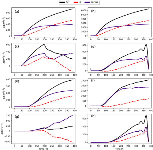
After this period, the potential vorticity variations overcome the effect of frontogenesis in altering the bulge stratification. This can be related to the complex recirculation of freshwater in the bulge which creates spirals of relative vorticity. The situation is different in the coastal current, where, over the duration of the simulation, frontogenesis remains the leading process (figure 24(e)).

The internal processes altering potential vorticity in the bulge and in the coastal current are evaluated in terms of potential vorticity budget. The contributions of advection, non-conservative processes (frictional and diabatic) and of boundary effects, to the temporal variation of potential vorticity, are examined here in both regions of the river plume (figure 25(a,e)).

Figure 25. Pv flux terms for (a) the Reference, (b) High discharge, (c) SW wind, (d) M2 Tide configurations in the bulge and for (e–h) same configurations in the coastal current. (Colour online)

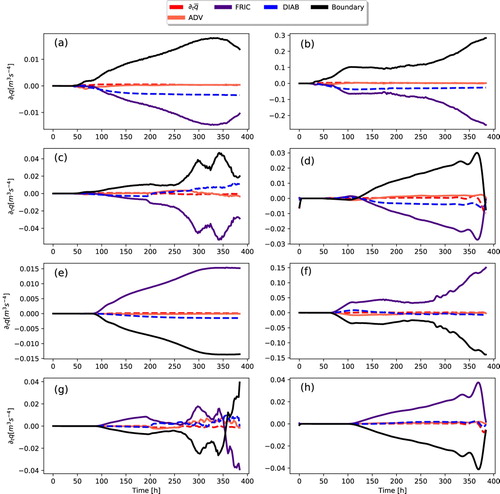
In a general case, frictional processes would be due to the surface wind stress, to unsteady and non-uniform forcings and to geostrophic current shears. In the absence of wind and of tide, the frictional flux of potential vorticity is essentially due to the velocity shear.

In the reference case, non-conservative processes (friction and diabatic mixing) contribute to reduce potential vorticity in the bulge. The frictional flux of potential vorticity is negative and is primarily due to the flow separation observed at early stages of the river plume evolution and to high velocity gradients in frontal region. Another non-conservative process is diabatic mixing which alters the strength of stratification. Here, we observe a buoyancy gain: stratification increases. The boundary value problem (BVP) term closes the budget as the volume of integration is time dependent. The BVP term indicates the advection of potential vorticity in the plume, along the bounding isopycnals.

In the reference case, the BVP term balances the non-conservative processes. In the bulge, it dominates the potential vorticity budget. By contrast, in the coastal current, non-conservative processes (among which, friction is chief) tend to reduce/destroy potential vorticity; but friction is balanced by the BVP term.

3.3.2. Sensitivity experiments

In the case of high discharge, the bulge stratification is primarily driven by frontogenesis during the first 8 days of the simulation, then by potential vorticity variations during the last 8 days (figure 24(b),(f)). In the coastal current, frontogenesis is the chief mechanism altering stratification. The order of magnitude of such processes is 10 times higher than in the reference case (moderate discharge). The kinetic energy density spectrum shows a $k^{-2}$ slope at the river plume base, corresponding to frontogenesis processes, and a $k^{-3}$ slope at the surface corresponding to quasi geostrophy (figure 10). The internal processes modifying potential vorticity in both the bulge and the coastal current, are also dominated by advection and mixing. Results comparable to those in the reference case are observed but with higher magnitude (figure 25(b,f)).

In the case of SW winds, stratification decreases after 8 days as does potential vorticity in the near field region while frontogenesis increases due to the mixing induced by winds (figure 24(c,g)). Meanwhile, in the coastal current, even with the presence of strong stratification, potential vorticity decreases while frontogenetic processes dominate over the integration time. A $k^{-2}$ slope characterises the kinetic energy spectrum at the surface and the river plume base which indicates the importance of frontogenesis in this case (figure 10).

Different processes can be distinguished for potential vorticity removal from or injection into the ocean interior (figure 25(c,g)). In the bulge, discharge and SW winds interact resulting in a negative diabatic potential vorticity flux, and a positive frictional flux. The negative diabatic flux indicates a surface buoyancy loss especially at the surface. Non-conservative processes are balanced by the BVP term. Interior potential vorticity variations are related to advection and the related shear. In the coastal current, a similar result is obtained as interior potential vorticity variations are governed by advective and shear processes. At the surface, friction plays an important role in potential vorticity removal in the coastal current.

When tides are taken into account, the variations in stratification are dominated by frontogenetic processes in both the bulge and the coastal current, over the entire simulation period (figure 24(d,h)). This latter diagnostic agrees with the $k^{-2}$ kinetic energy spectrum slope at the surface and at the river plume base (figure 10). In both river plume regions, the dominant process in the potential vorticity budget is advection and shear (figure 25(d,h)). In particular, stretching or squeezing of the water column and shear flows are generated by tidal oscillations. At the surface, friction plays an important role in the bulge, where vertical mixing of momentum is more intense.

4. Discussion

4.1. River plume hydrology and dynamics

In this paper, we studied the 3D structure and stability of a river plume. We addressed the impact of different forcings (discharge,wind and tide) on the plume (geostrophic or ageostrophic) dynamics.

Firstly, we observe the formation of an anticyclonic recirculating gyre (the bulge) once the freshwater enters the salty open ocean. In the absence of external forcings, the bulge grows in time, extending offshore. The bulge growth was considered by Nof and Pichevin (2001) or by Isobe (2005) as a ballooning effect due to the inertial recirculation. In the case of high discharge, its width and thickness increase significantly, due in part to the higher inflow velocities leading to instability at the edge of the bulge. In this frontal region, a layer with Rossby number $\mathrm{O}(1)$ indicates the presence of ageostrophic motions (Mcwilliams 1984, Voropayev and Filippov 1985). Spiraling filaments, with O(1) Rossby number and ageostrophic motions, then grow in the bulge core. Both the frontal region and the filaments grow when increasing the discharge. These filaments are due to the inner recirculation of bulge waters with different densities (different salinities). Indeed some of these waters have started mixing with seawater, while others are original estuarine waters. The dynamical adjustment of the bulge is associated with intensifying relative vorticity due to the continuous discharge (Spall and Price 1998). The simulated and idealised Gironde river plume in our study is similar to previous realistic studies in the Bay of Biscay regarding its radius (bulge radius) and freshwater thickness (Costoya et al. 2017).

A spatially uniform SW wind generates an Ekman transport which constrains the bulge to the coast; also the freshwater deepens near the coast, increasing the stratification (Fong and Geyer 2001, Lentz and Largier 2006). In the small bulge interior, strong ageostrophic motions are due to intense kinetic energy input; vertical vorticity and surface buoyancy fluxes are induced by the down front wind (Oort et al. 1994).

In the presence of a residual circulation of a M2 tide, the offshore growth of the bulge reaches an equilibrium between the influence of the tidal oscillations, and of the river discharge. The result is similar to that of Isobe (2005), who discussed the ballooning of the bulge and its stabilisation by tidal currents. Strong ageostrophic motions, near the estuary mouth, are due to periodic deformation (by flow and ebb) and to fluid column stretching and squeezing. This has been discussed in Maccready et al. (2002) using a conceptual model, and in Halverson and Pawlowicz (2008) using satellite imagery and in situ observations. They showed that turbulence remains close to the estuary mouth, for a river plume subject to tides during winter (well-mixed conditions).

Secondly, after few inertial periods a coastal current develops. In the absence of external forcings, the coastal current progresses to the north; it usually has half of the bulge width. This current grows with the unstable bulge as discussed in Horner-Devine (2009). The plume dynamics is geostrophic except at its external front (and sometimes along the coast) where strong ageostrophic motions can be observed (Yankovsky and Chapman 1997). In the case of downwelling favourable wind, the coastal current width is similar to the bulge width; this corresponds to an increase of northward freshwater transport (Chao 1987, 1988). As such a wind blows, the streamlines gets closer, due to Ekman transport, and the fluid is accelerated as a jet-like flow. This gives rise to strong ageostrophic circulation ($R_o\sim \mathrm{O}(1)$) in the frontal region (as explained in Thomas and Lee 2005; and in Choi and Wilkin 2007). When a tidal current is present, the coastal current is similar in shape and width to that in the reference case (case of moderate discharge). The coastal current is then in geostrophic balance (see also the studies by Guo and Valle-Levinson 2007, Hunter et al. 2010, Lai et al. 2016).

When we vary the parameters and physical effects acting on the plume, its modelled structure and dynamics evolves from that of the Gironde, to those of the Hudson and Columbia rivers (Hickey et al. 1998, Chant et al. 2008, Horner-Devine 2009).

4.2. River plume instabilities

To analyse the possible existence of plume instabilities (barotropic, baroclinic, Kelvin–Helmholtz, symmetric instabilities), we computed the energy transfer terms (HRS,VRS,VBF) from the eddy kinetic budget and the Rayleigh–Kuo, Charney–Stern and Hoskins criteria based on Ertel potential vorticity in isopycnic coordinates; we also evaluated the Richardson number. The use of isopycnic Ertel potential vorticity in this study is motivated by the need to adequately describe submesoscale and ageostrophic motions. Ertel potential vorticity differs from the quasi-geostrophic potential vorticity which is used for mesoscale dynamics studies (Rhines and Schopp 1991, Marshall and Adcroft 2010). Indeed the quasi-geostrophic approximation fails in frontal regions (regions of strong salinity/density gradients) and for intense motions (when Ro is O(1)).

We have shown the existence of different instabilities in the river plume. In the reference case (moderate discharge), instabilities are slowly growing. Increasing the river discharge intensifies instabilities. Using the Hoskins and Richardson number criteria, we have shown that symmetric instabilities develop near the surface in the bulge and in the coastal current. These instabilities coexist with baroclinic instability near the front, in particular in the bulge and with barotropic instability near the coast. At the northern edge of the coastal current, vertical shear and baroclinic instabilities coexist, as in the Mississippi river plume during periods of weak forcing (Hetland 2017). Symmetric instability will be replaced by baroclinic or barotropic ones when the Richardson number $R_i$ is $\mathrm{O}(1)$. Kelvin–Helmholtz instability can plays a stabilising role to symmetric instabilities, as shown via linear analysis in the Stone model (Stone 1966, Stamper and Taylor 2016).

In the case of SW winds (down-front winds), the wind induced shear and the flow shear give rise to all instabilities (barotropic, baroclinic, symmetric and Kelvin–Helmholtz) in the coastal current and in the small bulge. Winds aligned with the frontal velocity lead to frontal symmetric instability as suggested by D'Asaro et al. (2011). In this case, downfront winds catalyse energy release from the front to the surrounding turbulence. Baroclinic instability in the presence of downfront winds was previously shown by de Kok (1997), using a two-layer model. Baroclinically unstable conditions occur as the result of vertical velocity shear; this instability gives rise to frontal meanders with wavelengths between 18 and 30 km.

Finally, M2 Tides contribute to the rise of symmetric, barotropic and baroclinic instabilities in the near field region subject to intense turbulence. These instabilities can be due to the symmetrically unstable tidal front; this front becomes baroclinically and barotropically unstable near the estuary mouth. This result agrees with the results of the studies by Brink (2012, 2013). They show, using idealised simulations, that the existence of symmetric instabilities in tidal front is due to the sharpness of this latter and a well-mixed bottom boundary layer under the front. The growth of baroclinic instability in tidal fronts depends on bottom friction and topography slope.

Thus, during a typical winter, the Gironde river plume may undergo different instabilities but external forcings then play an important role. Yelekci (2017) showed, using realistic simulations, that baroclinic instabilities are dominant in the Gironde river plume, in winter. She attributed this instability to surface cooling which releases available potential energy leading to the deepening of the mixed layer depth.

4.3. River plume vertical mixing

Then the weakening or strengthening of the river plume have been investigated. Diapycnal or vertical mixing have been analysed via potential vorticity budget.

Firstly, we showed that frontogenesis and potential vorticity variations are important in altering the stratification. In the reference case (moderate discharge), the frontogenetic processes are important in the coastal current; they are induced by high strain at the edges of this latter. In the bulge, both frontogenetic and shear processes are important; potential vorticity variations are the strongest near the end of the simulation (about 10 days). A similar analysis (though with an order of magnitude stronger) was obtained for the high discharge case, except in the bulge, where potential vorticity variations overcome frontogenesis after 8 days. In the absence of wind stress and of tides, the frontogenesis contribution comes from the frontal region where high salinity gradients and ageostrophic motions are observed. In the absence of external forcings, the energy distribution is similar to that of quasi-geostrophic turbulence, in the bulge core at the surface, while ageostrophic effects dominate at the river plume base.

In the presence of down-front winds, the wind shear stress triggers frontogenetic process near the surface. In the small bulge, a submesoscale regime prevails. The downfront wind erodes potential vorticity while the frontogenetic processes induced by wind are important in both regions and particularly in the coastal current. In the presence of a residual tidal circulation, frontogenetic processes drive the changes in stratification in the whole river plume. This agrees with the $k^{-2}$ slope in energy spectrum, both at the bulge surface and base, in relation with submesoscale motions.

Secondly, we showed that the interior potential vorticity variations are controlled by differential advection. The Haynes and McIntyre impermeability theorem states that a balance is reached between non-conservative fluxes and the boundary value term (at bounding isopycnals). At the surface, velocity shear due to flow separation at the edges of the estuary, and friction related to vertical mixing of momentum in frontal regions are dominant. This explains the decay of potential vorticity in the coastal current in the presence of downwelling favourable winds. Indeed, stratification is altered by mixing associated with baroclinic instability and frontogenetic processes. Many atmospheric studies (Hoskins and Pedder 1980, Branscome et al. 1989, Barry et al. 2000) and oceanic studies (Lapeyre et al. 2006, Thomas and Ferrari 2008), in settings similar to ours, have shown similar results. Potential vorticity destruction by down-front winds has been analysed in Thomas (2005); they show that potential vorticity erosion is due to frictionless mixing. Frontogenetic processes are important at the edges of the plume, where strong cyclonic vorticity dominates. Therefore, we associate the cyclonic submesoscale ageostrophic circulation developed in the frontal region to frontogenetic processes induced by wind stirring or to shear and strained flow in general.

When tidal currents are present, ageostrophic motions dominate in the near field of the river plume subject to frontogenetic processes. These processes are key for restratification especially in tidal fronts. When strong tides act near the mouth of the Columbia River, sharp density and velocity fronts appear at the edges of the freshwater plume and perpendicularly to the coast; they result from frontogenetic processes during ebb tide cycles (Akan et al. 2017).

Frontogenesis in our study may also be compared to atmospheric straining at different levels of the atmosphere (Haynes and Shuckburgh 2000, Laîné et al. 2011).

5. Summary

The short time evolution of a Gironde-like river plume has been investigated. Idealised 3D numerical simulations have highlighted the dynamics of the river plume, and its instabilities. The bulge (the recirculating anticyclonic gyre) keeps growing in time in the absence of external forcings. This growth is limited by M2 tides and it is suppressed by downfront winds (southwesterly winds). After a few inertial periods, the coastal current is advected to the north with half of the bulge's width in the reference, high discharge and tidal forcing cases. In a system driven by downfront winds, the coastal current is the dominant feature with a jet-like outflow structure. The river plume dynamics is mainly geostrophically balanced except at the edges of the bulge and the coastal current (regions of strong salinity gradients) where ageostrophic motions are dominant.

The existence of numerous instabilities in different configurations has been highlighted. The (co)existence of baroclinic, barotropic, vertical shear instabilities and symmetric instabilities, with different combinations, is observed in the cases of high discharge and of downwelling favourable winds. Symmetric, baroclinic and barotropic instabilities co-exist in the near field region (close to the estuary mouth), in M2 tide case. The nature of these instabilities can be different in the frontal region where ageostrophic motions are important.

The stratification variations are due to potential vorticity advective mixing and frontogenetic processes. Frontogenetic processes can be dominant in cases of wind forcing or of tides but in different regions (far-field (wind forcing), near field (tidal forcing)). In the case of moderate or high discharge without any external forcings, both processes are important in the bulge, but in the far-field region, frontogenesis dominates largely.

Other effects can impact the geostrophic and ageostrophic dynamics and the mixing in a river plume. For example, turbulence in the ocean outside the plume, or the morphology of the estuary (as shown in Pimenta et al. 2011) or bottom friction (which can damp the development of instabilities – Brink 2013, Hetland 2017), can contribute to the river plume dynamics. They will be considered in a sequel of this study, with realistic numerical simulations.

Investigating the river plume dynamics at fine scales (with 200 m horizontal resolution) has shown the development of different instabilities, in various parts of the plume, and their sensitivity to external forcings. The vertical mixing in the river plume appears as resulting from a complex combination of frontogenesis and of non-conservative effects leading to variations of potential vorticity. These findings will be used in our next study to validate a realistic numerical simulation of the Gironde river plume in the Bay of Biscay, and to understand its instabilities and the vertical mixing affecting it.

Acknowledgments

This study is part of the COCTO project (SWOT science team program) funded by the CNES. The PhD Thesis of A. Ayouche is funded by Brittany region and Ifremer. Model simulations were carried out with GENCI (French National High-Performance Computing Organization) computational resources administered at the CINES (National Computing Center for Higher Education). The authors thank Bernard Le Cann and Robert Hetland for their fruitful advices and discussions. The authors thank Sabine Schmidt for providing the MAGEST in situ observations. MAGEST Verdon station was part of the DIAGIR project. The authors thank the two anonymous referees for their insightful and thoughtful comments.

Disclosure statement

No potential conflict of interest was reported by the author(s).

Additional information

Funding

This study is part of the COCTO project (SWOT science team program) funded by the CNES. The PhD Thesis of A. Ayouche is funded by Brittany region and Ifremer.

Appendix. Potential vorticity flux budget terms

We begin with the potential vorticity equation (A.1) ${\mathrm{\partial }}_{t}q=\mathrm{ADV}+\mathrm{FRIC}+\mathrm{DIAB}+\mathrm{Pres}.$(A.1) The different components can be expressed as (A.2) $\begin{array}{rl}\mathrm{ADV}& =(f+{\mathrm{\partial }}_{x}v-{\mathrm{\partial }}_{y}u){\mathrm{\partial }}_z(-\mathit{u}\mathbf{\cdot }\mathbf{\nabla }b)\\ & +{\mathrm{\partial }}_{z}b{\mathrm{\partial }}_x(-\mathit{v}\mathbf{\cdot }\mathbf{\nabla }\mathit{v}-fu)-{\mathrm{\partial }}_{z}b{\mathrm{\partial }}_y(-\mathit{u}\mathbf{\cdot }\mathbf{\nabla }\mathit{u}+fv)\\ & +{\mathrm{\partial }}_{y}b{\mathrm{\partial }}_z(-\mathit{u}\mathbf{\cdot }\mathbf{\nabla }\mathit{u}+fv)-{\mathrm{\partial }}_{x}b{\mathrm{\partial }}_z(-\mathit{v}\mathbf{\cdot }\mathbf{\nabla }\mathit{v}-fu)\\ & +{\mathrm{\partial }}_{z}u{\mathrm{\partial }}_y(-\mathit{u}\mathbf{\cdot }\mathbf{\nabla }b)-{\mathrm{\partial }}_{z}v{\mathrm{\partial }}_x(-\mathit{u}\mathbf{\cdot }\mathbf{\nabla }b),\end{array}$(A.2) (A.3) $\begin{array}{rl}\mathrm{FRIC}& ={\mathrm{\partial }}_{z}b[{\mathrm{\partial }}_x(\frac{\mathrm{D}v}{\mathrm{D}t}+\frac{1}{{\rho }_0}{\mathrm{\partial }}_{y}P+fu)-{\mathrm{\partial }}_y(\frac{\mathrm{D}u}{\mathrm{D}t}+\frac{1}{{\rho }_0}{\mathrm{\partial }}_{x}P-fv)]\\ & -{\mathrm{\partial }}_{y}b{\mathrm{\partial }}_z(\frac{\mathrm{D}u}{\mathrm{D}t}+\frac{1}{{\rho }_0}{\mathrm{\partial }}_{x}P-fv)-{\mathrm{\partial }}_{x}b{\mathrm{\partial }}_z(\frac{\mathrm{D}v}{\mathrm{D}t}+\frac{1}{{\rho }_0}{\mathrm{\partial }}_{y}P+fu),\end{array}$(A.3) (A.4) $\begin{array}{rl}\mathrm{DIAB}& =(f+{\mathrm{\partial }}_{x}v-{\mathrm{\partial }}_{y}u){\mathrm{\partial }}_z\left(\frac{\mathrm{D}b}{\mathrm{D}t}\right)+{\mathrm{\partial }}_{z}u{\mathrm{\partial }}_y\left(\frac{\mathrm{D}b}{\mathrm{D}t}\right)-{\mathrm{\partial }}_{z}v{\mathrm{\partial }}_x\left(\frac{\mathrm{D}b}{\mathrm{D}t}\right),\end{array}$(A.4) (A.5) $\begin{array}{rl}\mathrm{Pres}& ={\mathrm{\partial }}_{z}b[{\mathrm{\partial }}_x\left(\frac{1}{{\rho }_0}{\mathrm{\partial }}_{y}P\right)-{\mathrm{\partial }}_y\left(\frac{1}{{\rho }_0}{\mathrm{\partial }}_{x}P\right)]-{\mathrm{\partial }}_{y}b{\mathrm{\partial }}_z\left(\frac{1}{{\rho }_0}{\mathrm{\partial }}_{x}P\right)-{\mathrm{\partial }}_{x}b{\mathrm{\partial }}_z\left(\frac{1}{{\rho }_0}{\mathrm{\partial }}_{y}P\right),\end{array}$(A.5) where $\mathrm{D}/\mathrm{D}t={\mathrm{\partial }}_t+\mathit{u}\mathbf{\cdot }\mathbf{\nabla }$.

Now, we integrate the potential vorticity equation (A.1(A.1) ${\mathrm{\partial }}_{t}q=\mathrm{ADV}+\mathrm{FRIC}+\mathrm{DIAB}+\mathrm{Pres}.$(A.1) ) over a volume varying in time (A.6) ${\mathrm{\partial }}_t{\int }_{V(t)}q\mathrm{d}V={\int }_{V(t)}(\mathrm{ADV}+\mathrm{FRIC}+\mathrm{DIAB}+\mathrm{Pres})\mathrm{d}V+\mathrm{BVP},$(A.6) where (A.7) $\mathrm{BVP}={\int }_{A(t)}q{\mathit{u}}_{\mathit{A}}\mathbf{\cdot }\mathrm{d}\mathit{A}$(A.7) is the lateral boundary values here the bounding isopycnes. Further, ${\mathit{u}}_A$ is the velocity along the bounding isopycnes and $\mathit{A}$ is the bounding surface.

References

- Akan, C., Moghimi, S., Ozkan-Haller, H.T., Osborne, J. and Kurapov, A., On the dynamics of the mouth of the Columbia river: Results from a three-dimensional fully coupled wave-current interaction model. J. Geophys. Res. Oceans 2017, 122, 5218–5236.
- Avicola, G. and Huq, P., Scaling analysis for the interaction between a buoyant coastal current and the continental shelf: Experiments and observations. J. Phys. Oceanogr. 2002, 32, 3233–3248.
- Barry, L., Craig, G. and Thuburn, J., A GCM investigation into the nature of baroclinic adjustment. J. Atmos. Sci. 2000, 57, 1141–1155.
- Botas, J., Fernández, E., Bode, A. and Anadón, R., A persistent upwelling off the Central Cantabrian Coast (Bay of Biscay). Estuar. Coast. Shelf Sci. 1990, 30, 185–199.
- Branscome, L., Gutowski, W. and Stewart, D., Effect of surface fluxes on the nonlinear development of baroclinic waves. J. Atmos. Sci. 1989, 46, 460–475.
- Brink, K., Baroclinic instability of an idealized tidal mixing front. J. Marine Res. 2012, 70, 661–688.
- Brink, K., Instability of a tidal mixing front in the presence of realistic tides and mixing. J. Marine Res. 2013, 71, 227–252.
- Caballero, A., Ferrer, L., Rubio, A., Charria, G., Taylor, B.H. and Grima, N., Monitoring of a quasi-stationary eddy in the Bay of Biscay by means of satellite, in situ and model results. Deep-Sea Res. Pt. II-Top. Stud. Oceanogr. 2014, 106, 23–37. Oceanography of the Bay of Biscay.
- Callendar, W., Klymak, J.M. and Foreman, M.G.G., Tidal generation of large sub-mesoscale eddy dipoles. Ocean Sci. 2011, 7, 487–502.
- Capuano, T., Sabrina, S., Xavier, C. and Blanke, B., Mesoscale and submesoscale processes in the Southeast Atlantic and their impact on the regional thermohaline structure. J. Geophys. Res. Oceans 2018, 123, 1937–1961.
- Castaing, P., Courantologie de dérive dans les zones côtières á l'aide de bouées positionnées par satellite (Système ARGOS), in Proceedings of XVIIIème Journées de l'hydraulique. Marseille, 1984, pp. I.4.1–I.4.8.
- Chant, R., Wilkin, J., Zhang, W., Choi, B.J., Hunter, E., Castelao, R., Glenn, S., Jurisa, J., Schofield, O., Houghton, R., Kohut, J., Frazer, T. and Moline, M., Dispersal of the Hudson river plume in the New York Bight: Synthesis of observational and numerical studies during LaTTE. Biol. Sci. 2008, 21, 148–161.
- Chao, S.Y., Wind-driven motion near inner shelf fronts. J. Geophys. Res. Oceans 1987, 92, 3849–3860.
- Chao, S.Y., Wind-driven motion of estuarine plumes. J. Phys. Oceanogr. 1988, 18, 1144–1166.
- Chapman, D.C., Numerical treatment of cross-shelf open boundaries in a barotropic coastal ocean model. J. Phys. Oceanogr. 1985, 15, 1060–1075.
- Charria, G., Lazure, P., Cann, B.L., Serpette, A., Reverdin, G., Louazel, S., Batifoulier, F., Dumas, F., Pichon, A. and Morel, Y., Surface layer circulation derived from Lagrangian drifters in the Bay of Biscay. J. Marine Syst. 2013, 109–110, S60–S76. XII International Symposium on Oceanography of the Bay of Biscay.
- Choi, B.J. and Wilkin, J.L., The effect of wind on the dispersal of the Hudson river plume. J. Phys. Oceanogr. 2007, 37, 1878–1897.
- Costoya, X., Fernández-Nóvoa, D. and Gómez-Gesteira, M., Loire and Gironde turbid plumes: Characterization and influence on thermohaline properties. J. Sea Res. 2017, 130, 7–16. Changing Ecosystems in the Bay of Biscay: Natural and Anthropogenic Effects.
- D'Asaro, E., Lee, C., Rainville, L., Harcourt, R. and Thomas, L., Enhanced turbulence and energy dissipation at ocean fronts. Science 2011, 332, 318–322.
- de Kok, J., Baroclinic eddy formation in a Rhine plume model. J. Marine Syst. 1997, 12, 35–52.
- Debreu, L., Marchesiello, P., Penven, P. and Cambon, G., Two-way nesting in split-explicit ocean models: algorithms, implementation and validation. Ocean Model. 2012, s 49–50, 1–21.
- Ertel, H., Ein neuer hydrodynamischer Erhaltungssatz. Naturwissenschaften 1942, 30, 543–544.
- Evans Contreras, M., Pizarro, O., Dewitte, B., Sepúlveda, H. and Renault, L., Subsurface mesoscale eddy generation in the ocean off central Chile. J. Geophys. Res. Oceans 2019, 124, 5700–5722.
- Fong, D.A. and Geyer, W.R., Response of a river plume during an upwelling favorable wind event. J. Geophys. Res. Oceans 2001, 106, 1067–1084.
- Garvine, R.W., Penetration of buoyant coastal discharge onto the continental shelf: A numerical model experiment. J. Phys. Oceanogr. 1999, 29, 1892–1909.
- Gohin, F., Annual cycles of chlorophyll-a, non-algal suspended particulatematter, and turbidity observed from space and in-situ incoastal waters. Ocean Sci. 2011, 7, 705–732.
- Gröbelbauer, H.P., Fanneløp, T.K. and Britter, R.E., The propagation of intrusion fronts of high density ratios. J. Fluid Mech. 1993, 250, 669–687.
- Gula, J., Molemaker, M. and Mcwilliams, J., Topographic generation of submesoscale centrifugal instability and energy dissipation. Nat. Commun. 2016, 7, 12811.
- Guo, X. and Valle-Levinson, A., Tidal effects on estuarine circulation and outflow plume in the Chesapeake Bay. Cont. Shelf Res. 2007, 27, 20–42.
- Halverson, M.J. and Pawlowicz, R., Estuarine forcing of a river plume by river flow and tides. J. Geophys. Res. Oceans 2008, 113, C09033.
- Haynes, P. and Shuckburgh, E., Effective diffusivity as a diagnostic of atmospheric transport: 1. Stratosphere. J. Geophys. Res. Atmos. 2000, 105, 22777–22794.
- Hetland, R.D., Relating river plume structure to vertical mixing. J. Phys. Oceanogr. 2005, 35, 1667–1688.
- Hetland, R.D., Suppression of baroclinic instabilities in buoyancy-driven flow over sloping bathymetry. J. Phys. Oceanogr. 2017, 47, 49–68.
- Hickey, B.M., Pietrafesa, L.J., Jay, D.A. and Boicourt, W.C., The Columbia river plume study: Subtidal variability in the velocity and salinity fields. J. Geophys. Res. Oceans 1998, 103, 10339–10368.
- Horner-Devine, A., The bulge circulation in the Columbia river plume. Cont. Shelf Res. 2009, 29, 234–251.
- Horner-Devine, A.R., Hetland, R.D. and MacDonald, D.G., Mixing and transport in coastal river plumes. Ann. Rev. Fluid Mech. 2015, 47, 569–594.
- Hoskins, B., The role of potential vorticity in symmetric stability and instability. Q. J. R. Meteor. Soc. 1974, 100, 480–482.
- Hoskins, B.J. and Pedder, M.A., The diagnosis of middle latitude synoptic development. Q. J. R. Meteor. Soc. 1980, 106, 707–719.
- Hunter, E.J., Chant, R.J., Wilkin, J.L. and Kohut, J., High-frequency forcing and subtidal response of the Hudson river plume. J. Geophys. Res. Oceans 2010, 115, 1–16.
- Isobe, A., Ballooning of river-plume bulge and its stabilization by tidal currents. J. Phys. Oceanogr. 2005, 35, 2337–2351.
- Iwanaka, Y. and Isobe, A., Tidally induced instability processes suppressing river plume spread in a nonrotating and nonhydrostatic regime. J. Geophys. Res. Oceans 2018, 123, 3545–3562.
- Kang, D., Energetics of eddy-mean flow interactions in the gulf stream region. J. Phys. Oceanogr. 2015, 45, 1103–1120.
- Kantha, L.H. and Clayson, C.A., An improved mixed layer model for geophysical applications. J. Geophys. Res. Oceans 1994, 99, 25235–25266.
- Kelly-Gerreyn, B., Hydes, D., Jégou, A., Lazure, P., Fernand, L., Puillat, I. and Garcia-Soto, C., Low salinity intrusions in the western English channel. Cont. Shelf Res. 2006, 26, 1241–1257.
- Kilcher, L.F. and Nash, J.D., Structure and dynamics of the Columbia river tidal plume front. J. Geophys. Res.-Oceans 2010, 115, C05S90.
- Lai, Z., Ma, R., Huang, M., Chen, C., Chen, Y., Xie, C. and Beardsley, R.C., Downwelling wind, tides, and estuarine plume dynamics. J. Geophys. Res. Oceans 2016, 121, 4245–4263.
- Laîné, A., Lapeyre, G. and Rivière, G., A quasigeostrophic model for moist storm tracks. J. Atmos. Sci. 2011, 68, 1306–1322.
- Lapeyre, G., Klein, P. and Hua, B.L., Oceanic restratification forced by surface frontogenesis. J. Phys. Oceanogr. 2006, 36, 1577–1590.
- Lavín, A., Valdès, L., Sánchez, F., Abaunza, P., Forest, A., Boucher, J., Lazure, P. and Jegou, A., The Bay of Biscay: the encountering of the ocean and the shelf. In The Sea. Volume 14. Part B. The Global Coastal Ocean: Interdisciplinary Regional Studies and Synthesis, edited by A. Robinson and K. Brink, chap. 24, pp. 933–999, 2006 (Harvard University Press: Harvard).
- Lazure, P., Garnier, V., Dumas, F., Herry, C. and Chifflet, M., Development of a hydrodynamic model of the Bay of Biscay. Validation of hydrology. Cont. Shelf Res. 2009, 29, 985–997. 100 Years of Research within the Bay of Biscay.
- Lazure, P. and Jegou, A.M., 3D modelling of seasonal evolution of Loire and Gironde plumes on Biscay Bay continental shelf. Oceanol. Acta 1998, 21, 165–177. International Conference on Oceanography of the Bay of Biscay.
- Le Boyer, A., Charria, G., Le Cann, B., Lazure, P. and Marié, L., Circulation on the shelf and the upper slope of the Bay of Biscay. Cont. Shelf Res. 2013, 55, 97–107.
- Lentz, S.J. and Helfrich, K.R., Buoyant gravity currents along a sloping bottom in a rotating fluid. J. Fluid Mech. 2002, 464, 251–278.
- Lentz, S. and Largier, J., The influence of wind forcing on the Chesapeake Bay buoyant coastal current*. J. Phys. Oceanogr. 2006, 36, 1305–1316.
- Li, M. and Rong, Z., Effects of tides on freshwater and volume transports in the Changjiang river plume. J. Geophys. Res.-Oceans 2012, 117, C06027.
- Lowe, R.J., Rottman, J.W. and Linden, P.F., The non-Boussinesq lock-exchange problem. Part 1. Theory and experiments. J. Fluid Mech. 2005, 537, 101–124.
- Maccready, P., Hetland, R. and Geyer, W., Long-term isohaline salt balance in an estuary. Cont. Shelf Res. 2002, 22, 1591–1601.
- MacDonald, D.G. and Geyer, W.R., Turbulent energy production and entrainment at a highly stratified estuarine front. J. Geophys. Res. Oceans 2004, 109, C05004.
- Marchesiello, P., McWilliams, J.C. and Shchepetkin, A., Open boundary conditions for long-term integration of regional oceanic models. Ocean Model. 2001, 3, 1–20.
- Marshall, D.P. and Adcroft, A.J., Parameterization of ocean eddies: Potential vorticity mixing, energetics and Arnold's first stability theorem. Ocean Model. 2010, 32, 188–204. The magic of modelling: A special volume commemorating the contributions of Peter D. Killworth – Part 2.
- Marshall, J., Jamous, D. and Nilsson, J., Entry, flux, and exit of potential vorticity in ocean circulation. J. Phys. Oceanogr. 2001, 31, 777–789.
- Marshall, J.C. and Nurser, A.J.G., Fluid dynamics of oceanic thermocline ventilation. J. Phys. Oceanogr. 1992, 22, 583–595.
- Mcwilliams, J.C., The emergence of isolated coherent vortices in turbulent flow. J. Fluid Mech. 1984, 146, 21–43.
- McWilliams, J.C., Submesoscale currents in the ocean. Proc. R. Soc. A–Math. Phys. Eng. Sci. 2016, 472, 20160117.
- Morel, Y. and McWilliams, J., Effects of isopycnal and diapycnal mixing on the stability of oceanic currents. J. Phys. Oceanogr. 2001, 31, 2280–2296.
- Nash, J., Kilcher, L. and Moum, J., Structure and composition of a strongly stratified, tidally pulsed river plume. J. Geophys. Res. 2009, 114, C00B12.
- Nof, D. and Pichevin, T., The ballooning of outflows. J. Phys. Oceanogr. 2001, 31, 3045–3058.
- O'Donnell, J., The dynamics of estuary plumes and fronts. In Contemporary Issues in Estuarine Physics, edited by A. Valle-Levinson, chap. 8, pp. 186–246, 2010 (Cambridge University Press: Cambridge).
- Oort, A.H., Anderson, L.A. and Peixoto, J.P., Estimates of the energy cycle of the oceans. J. Geophys. Res. Oceans 1994, 99, 7665–7688.
- Orlanski, I., A simple boundary condition for unbounded hyperbolic flows. J. Comp. Phys. 1976, 21, 251–269.
- Palma, E. and Matano, R., An idealized study of near equatorial river plumes. J. Geophys. Res. Oceans 2017, 122, 3599–3620.
- Pan, J. and Jay, D., Effects of ambient velocity shear on nonlinear internal wave associated mixing at the Columbia river plume front. J. Geophys. Res. 2009, 114, C00B07.
- Pimenta, F., Kirwan, A. and Huq, P., On the transport of buoyant coastal plumes. J. Phys. Oceanogr. 2011, 41, 620–640.
- Pingree, R.D. and Le Cann, B., Structure, strength and seasonality of the slope currents in the Bay of Biscay region. J. Mar. Bio. Assoc. UK 1990, 70, 857–885.
- Pingree, R. and Sinha, B., Westward moving waves or eddies (Storms) on the subtropical/azores front near 32.5∘N? interpretation of the eulerian currents and temperature records at moorings 155 (35.5∘W) and 156 (34.4∘W). J. Marine Syst. 2001, 29, 239–276.
- Puillat, I., Lazure, P., Jégou, A., Lampert, L. and Miller, P., Hydrographical variability on the French continental shelf in the Bay of Biscay, during the 1990s. Cont. Shelf Res. 2004, 24, 1143–1163.
- Rathan, S. and Raju, G.N., A modified fifth-order WENO scheme for hyperbolic conservation laws. Comput. Math. Appl. 2018, 75, 1531–1549.
- Rhines, P. and Schopp, R., The wind-driven circulation: Quasi-geostrophic simulations and theory for nonsymmetric winds. J. Phys. Oceanogr. 1991, 21, 1438–1469.
- Rubio, A., Caballero, A., Orfila, A., Hernández-Carrasco, I., Ferrer, L., González, M., Solabarrieta, L. and Mader, J., Eddy-induced cross-shelf export of high Chl-a coastal waters in the SE Bay of Biscay. Remote Sens. Environ. 2018, 205, 290–304.
- Schiller, R.V., Kourafalou, V.H., Hogan, P. and Walker, N.D., The dynamics of the Mississippi River plume: Impact of topography, wind and offshore forcing on the fate of plume waters. J. Geophys. Res. Oceans 2011, 116, C06029.
- Schubert, W., Ruprecht, E., Hertenstein, R., Ferreira, R.N., Taft, R., Rozoff, C., Ciesielski, P. and Kuo, H.C., English translations of twenty-one of Ertel's papers on geophysical fluid dynamics. Meteorol. Z. 2004, 13, 527–576.
- Shchepetkin, A. and McWilliams, J., The regional oceanic modeling system (ROMS): A split-explicit, free-surface, topography-following- coordinate ocean model. Ocean Model. 2005, 9, 347–404.
- Sheng, J., Dynamics of a buoyancy-driven coastal jet: The Gaspé current. J. Phys. Oceanogr. 2001, 31, 3146–3162.
- Simpson, J., Brown, J., Matthews, J. and Allen, G., Tidal straining, density currents, and stirring in the control of estuarine stratification. Estuaries 1990, 13, 125–132.
- Spall, M. and Price, J., Mesoscale variability in Denmark strait: The PV outflow hypothesis. J. Phys. Oceanogr. 1998, 28, 1598–1623.
- Stamper, M. and Taylor, J., The transition from symmetric to baroclinic instability in the Eady model. Ocean Dyn. 2016, 67, 65–80.
- Stone, P.H., On non-geostrophic baroclinic stability. J. Atmos. Sci. 1966, 23, 390–400.
- Teles-Machado, A., Peliz, A., McWilliams, J.C., Cardoso, R.M., Soares, P.M.M. and Miranda, P.M.A., On the year-to-year changes of the Iberian Poleward current. J. Geophys. Res. Oceans 2015, 120, 4980–4999.
- Thomas, L.N., Destruction of potential vorticity by winds. J. Phys. Oceanogr. 2005, 35, 2457–2466.
- Thomas, L. and Ferrari, R., Friction, frontogenesis, and the stratification of the surface mixed layer. J. Phys. Oceanogr. 2008, 38, 2501–2518.
- Thomas, L.N. and Lee, C.M., Intensification of ocean fronts by down-front winds. J. Phys. Oceanogr. 2005, 35, 1086–1102.
- Thomas, L., Tandon, A. and Mahadevan, A., Submesoscale Processes and Dynamics. Geophysical Monograph Series, Vol. 177, 2008. (Washington, DC: American Geophysical Union).
- Thomas, L., Taylor, J., Ferrari, R. and Joyce, T., Symmetric instability in the Gulf stream. Deep-Sea Res. Pt. II-Top. Stud. Oceanogr. 2013, 91, 96–110.
- Umlauf, L. and Burchard, H., Second-order turbulence closure models for geophysical boundary layers. A review of recent work. Cont. Shelf Res. 2005, 25, 795–827.
- Vandermeirsch, F., Charraudeau, M., Bonnat, A., Fichaut, M., Maillard, C., Gaillard, F. and Autret, E., Bay of Biscay's temperature and salinity climatology, in XII International Symposium on Oceanography of the Bay of Biscay, 4–6 mai 2010, Plouzané, France, 2010.
- Vic, C., Berger, H., Treguier, A.M. and Couvelard, X., Dynamics of an equatorial river plume: Theory and numerical experiments applied to the Congo plume case. J. Phys. Oceanogr. 2014, 44, 940.
- Visser, A., Souza, A., Hessner, K. and Simpson, J., The influence of water column stratification on tidal current profile in a ROFI system. Oceanol. Acta 1994, 17, 369–381.
- Voropayev, S. and Filippov, I., Development of a horizontal jet in homogeneous and stratified fluids. Laboratory experiment. J. Fluid Mech. 1985, 21, 964–972.
- Walters, R.A. and Heston, C., Removing tidal-period variations from time-series data using low-pass digital filters. J. Phys. Oceanogr. 1982, 12, 112–115.
- Warner, J.C., Geyer, W.R. and Lerczak, J.A., Numerical modeling of an estuary: A comprehensive skill assessment. J. Geophys. Res. Oceans 2005, 110, C05001.
- Yankovsky, A. and Chapman, D., A simple theory for the fate of buoyant coastal discharges. J. Phys. Oceanogr. 1997, 27, 1386–1401.
- Yelekci, O., Submesoscale dynamics in the Bay of Biscay continental shelf. Ph.D. Thesis, Pierre and Marie-Curie University 2017PA066529, 2017.