Formation of small-scale vortices in the core of a large merged vortex

Abstract

The merger of two surface quasi-geostrophic vortices is examined in detail. As the two vortices collapse towards each other in the merging process, they trap their external fronts between them; these fronts are inserted into the final merged vortex, where they form a central, nearly parallel, sheared velocity strip, sensitive to barotropic instability. As a result, this strip breaks up into an alley of small vortices. Subsequently, these small vortices may undergo merger and grow in size in the core of the large merged vortex. The number of small trapped vortices decreases correspondingly. Finally, a single or two small vortices remain. These processes are analysed using a numerical model of the surface quasi-geostrophic equations. The sensitivity of this process to the initial vortex characteristics is explored. A parallel is drawn between this problem and the instability of a rectilinear strip of temperature with a central gap. The application of this problem to the Ocean is discussed.

Keywords:

• Surface quasi-geostrophy
• vortex merger
• barotropic instability
• small vortices
• core trapping

1. Context and motivation

Vortices are long-lived structures with internally recirculating fluid, of paramount importance in the oceanic and atmospheric flows. They carry a substantial part of the energy, momentum, heat and tracers released by the large-scale, wind-driven currents, see Zhang et al. (2014). When vortices are generated in a small domain, their initial proximity allows their strong mutual interactions. Among the possible interactions, vortex merger is the process by which two initially close, like-signed, vortices collapse towards each other and form a larger vortex, see Saffman and Szeto (1980), Overman II and Zabusky (1982), Melander et al. (1988), and Brandt and Nomura (2006). This process has been studied at length in geophysical fluid dynamics, see Cresswell (1982), Capéran and Verron (1988), Pavia and Cushman-Roisin (1990), Verron et al. (1990), Verron and Hopfinger (1991), Carton (1992), Hopfinger and van Heijst (1993), Valcke and Verron (1993, 1996, 1997), Verron and Valcke (1994), von Hardenberg et al. (2000), Sokolovskiy and Verron (2000), Dritschel (2002), Reinaud and Dritschel (2002, 2005), Bambrey et al. (2007), Ozugurlu et al. (2008), Sokolovskiy and Verron (2014), Ciani et al. (2016), Carton et al. (2017), Sokolovskiy et al. (2018), and Reinaud and Dritschel (2019), as it is central to the growth of vortices in the Ocean, and to their resistance to erosion, see Legras and Dritschel (2001), Carton et al. (2017), and Morvan et al. (2019).

Among the various systems of equations of relevance to oceanic fluid dynamics, the surface quasi-geostrophy (SQG) model is well adapted to describe the evolution of medium and small scale vortices, see Held et al. (1995). The SQG equations govern the evolution of a buoyancy anomaly on a flat surface (here the Ocean's surface). They also provide the relation between the buoyancy distribution and the flow that it generates. The former equation is a hyperbolic partial differential equation while the latter is an elliptic equation. It should also be noted that the two-dimensional distribution of buoyancy at the ocean surface creates a three-dimensional flow field which extends into the depth of the ocean. For the purpose of the present study, nevertheless, we only consider the flow field at the sea surface and we investigate how it advects the buoyancy anomalies.

In the SQG model, vortex merger has been studied and shown to produce large vortices, external filaments and small scale debris of buoyancy anomalies (Carton et al. 2016). The production of both these larger-scale vortices and small scale features feeds a dual direct and inverse energy cascade and is a consequence of the conservation of flow invariants during the merger (see, e.g. Reinaud and Dritschel 2002). By carefully re-examining this process, we show in the present study that internal fronts are also formed, that is, fronts in the core of the finally merged vortex. These inner fronts are unstable and break up into a vortex alley. The small vortices thus formed inside the main merged vortex are close to each other and merge to form larger inner vortices. Overall, this process yields a large vortex with one or two smaller vortices in its core, similar to what is now observed with high-resolution measurements of oceanic vortices.

The paper proceeds as follows: section 2 presents the SQG equations and their numerical implementation. Subsection 3.1 describes the merger of two SQG vortices at high-resolution and shows the trapping of buoyancy fronts in the core. These inner fronts are unstable. The linear stability of a model of a parallel front in presented in subsection 3.2, and its nonlinear evolution in subsection 3.2.2. In subsection 3.3, a nonlinear numerical simulation shows the breaking of the front into small vortices and their subsequent evolution during the merger of two vortices. The results are then discussed in view of oceanic vortex observations and of previous work in section 4.

2. Surface quasi-geostrophic equations and numerical model

The SQG equations read (1) $\begin{array}{rlrl}{\mathrm{\partial }}_t\Theta +J(\psi ,\Theta )& =0,& \mathrm{on}z& =0,\end{array}$(1) (2) $\begin{array}{rlrl}\Theta & =-{\mathrm{\partial }}_z\psi ,& \mathrm{on}z& =0\end{array}$(2) (3) $\begin{array}{rlrl}\mathrm{\Delta }\psi & =0,& \mathrm{for}z& \le 0,\end{array}$(3) (4) $\begin{array}{rlrl}\psi & \to 0,& \mathrm{as}z& \to -\mathrm{\infty },\end{array}$(4) where $\Theta$ is potential temperature, or equivalently the buoyancy anomaly in the Ocean, and ψ is the streamfunction. In equation (3(3) $\begin{array}{rlrl}\mathrm{\Delta }\psi & =0,& \mathrm{for}z& \le 0,\end{array}$(3) ), Δ is the three-dimensional Laplacian. We study the evolution of $\Theta$ and ψ as functions of x, y, t, at the surface z = 0. In equation (1(1) $\begin{array}{rlrl}{\mathrm{\partial }}_t\Theta +J(\psi ,\Theta )& =0,& \mathrm{on}z& =0,\end{array}$(1) ), J is the Jacobian operator defined as $J(a,b)={\mathrm{\partial }}_{x}a{\mathrm{\partial }}_{y}b-{\mathrm{\partial }}_{x}b{\mathrm{\partial }}_{y}a$. Using (3(3) $\begin{array}{rlrl}\mathrm{\Delta }\psi & =0,& \mathrm{for}z& \le 0,\end{array}$(3) ), equation (2(2) $\begin{array}{rlrl}\Theta & =-{\mathrm{\partial }}_z\psi ,& \mathrm{on}z& =0\end{array}$(2) ) becomes (5) $\Theta =-(-{\mathrm{\Delta }}_h{)}^{1/2}\psi ,$(5) where ${\mathrm{\Delta }}_h$ is the horizontal Laplacian. Equation (1(1) $\begin{array}{rlrl}{\mathrm{\partial }}_t\Theta +J(\psi ,\Theta )& =0,& \mathrm{on}z& =0,\end{array}$(1) ) is hyperbolic, while equation (5(5) $\Theta =-(-{\mathrm{\Delta }}_h{)}^{1/2}\psi ,$(5) ) is elliptic. The Green's function associated with the linear operator in (5(5) $\Theta =-(-{\mathrm{\Delta }}_h{)}^{1/2}\psi ,$(5) ) is $G(r)=1/(2\pi r)$, indicating that the flow field created by a buoyancy distribution is intense at short range.

The fluid domain is assumed periodic in both the x and $y-$directions and of dimension $2\pi \times 2\pi$. Equation (1(1) $\begin{array}{rlrl}{\mathrm{\partial }}_t\Theta +J(\psi ,\Theta )& =0,& \mathrm{on}z& =0,\end{array}$(1) ) is marched in time using a mixed Euler-leapfrog scheme. Equation (5(5) $\Theta =-(-{\mathrm{\Delta }}_h{)}^{1/2}\psi ,$(5) ) is solved in spectral space. The horizontal resolution is set to $512\times 512$ for sensitivity studies and to $1024\times 1024$ for the reference simulation. Bi-harmonic viscosity is used to eliminate the usual buoyancy accumulation at small scales, but it is kept to the minimal value required to ensure the numerical stability of the numerical model. The initial conditions of the model consist of two identical, non-overlapping vortices. Each vortex is initially circular, with radius R = 0.5 and its profile is either a top-hat or is smooth, defined by $\theta (r)=\sqrt{1-r/R},r<R,,\theta (r)=0,>R$. For the top-hat vortices, the edge of the vortices is locally smoothed to avoid a discontinuity. The two vortex centres are initially separated by a distance d>2R.

For the analysis of numerical results, we define the Okubo-Weiss quantity (Okubo 1970, Weiss 1991) (6) $OW={\sigma }^2-{\zeta }^2,$(6) with (7) $\begin{array}{r}{\sigma }^2={\sigma }_1^2+{\sigma }_2^2=({\mathrm{\partial }}_{x}u-{\mathrm{\partial }}_{y}v{)}^2+({\mathrm{\partial }}_{x}v+{\mathrm{\partial }}_{y}u{)}^2,\\ \zeta ={\mathrm{\partial }}_{x}v-{\mathrm{\partial }}_{y}u,D={\mathrm{\partial }}_{x}u+{\mathrm{\partial }}_{y}v=0.\end{array}$(7) In regions where OW>0, the straining field is more intense than the vorticity, and kinematically, vortices become more deformed and tend to shed filaments. The increase in temperature gradients is measured by the frontogenetic function FGT which obeys (8) $\frac{\mathrm{d}}{\mathrm{d}t}\left(\frac{1}{2}|\mathbf{\nabla }T{|}^2\right)=FGT,$(8) with (9) $FGT=(\mathbf{\nabla }T\mathbf{\cdot }\mathbf{\nabla }\mathit{u})\mathbf{\nabla }T.$(9)

3. Results

In this section, we describe the evolution of the two vortices in 3 stages:

1. the initial collapse of the two vortices towards each other (and towards the centre of the domain) leading to the amplification of the temperature front between them, which is then trapped into the merged vortex,

2. the adjustment of the merged vortex (its oscillation) and the destabilisation of this internal front,

3. the formation of small vortices in the large vortex core and their subsequent evolution; in this last part, we will also discuss the presence of small vortices in other parts of the flow field.

3.1. Initial merger of two large vortices

Firstly, we performed a set of numerical simulations of the interaction of a pair of top-hat vortices at $512\times 512$ resolution with minimal bi-harmonic viscosity (${\nu }_4=2{10}^{-14}$ in dimensionless value) and varying d/R (figures not shown). These simulations allow one to determine the critical merger distance for the vortex pair. Indeed, vortices collapse towards each other and merge only if the distance separating them is less than a threshold known as the critical merger distance. This first set of simulations shows that, for an initial separation $d/R\le 2.8$, the two vortices merge very rapidly (in less than one-half global turnover time) and irreversibly. For $d/R=2.9$, the two vortices merge, separate and finally merge again to form a very elongated quasi-elliptical vortex which oscillates with several modes of deformation (in particular, an azimuthal mode 4, which is the first harmonic of the main elliptical mode of deformation of the merged vortex). For $d/R=3.0$, the two vortices touch near the centre of the plane, while co-rotating. They merge, separate, merge again and finally separate. For $d/R=3.1$, the two vortices do not merge. Therefore, the merger and non merger regimes are connected by a regime of successive mergers and separations. This is generic of vortex merger. It can be noted that increasing the viscosity favours merger. In particular, for ${\nu }_4={10}^{-12}$, the regimes are shifted by 0.1 in d/R (e.g. the former evolution at $d/R=3.0$ now occurs at $d/R=2.9$). It is known that, when the flow becomes viscous enough, all vortices spread out and finally merge. We ascertain here not to enter this fully viscous regime and we consider only dynamical merger (for which the vortices merge within less than a global turnover period).

Following this first result, we next further investigate the merger of the two top-hat vortices for $d/R=2.5$ at t = 0 so that the vortices fully merge rapidly. We increase the model resolution to $1024\times 1024$. Our bi-harmonic viscosity can be decreased down to ${\nu }_4={10}^{-15}$ which is the minimal value ensuring numerical stability while not perturbing the physical result of the model. Figure 1 presents the evolution of the temperature maps. Clearly, the external temperature fronts are trapped in the core of the merged vortex. This front forms a strip in the middle of the merged S-shaped vortex (see the subplot at time t = 3). This front is associated with a strong velocity shear.

Figure 1. Series of temperature maps in the $(x,y)$-plane at t = 0, 3, 4.5, 9, 12, 15 illustrating the formation of a row of small vortices at the centre of the merged vortex for $d/R=2.5$ at resolution $1024\times 1024$. The black lines denote the contours of various temperature levels between 0 and 1. (a) t = 0.0. (b) t = 3.0. (c) t = 4.5. (d) t = 9. (e) t = 12 and (f) t = 15.

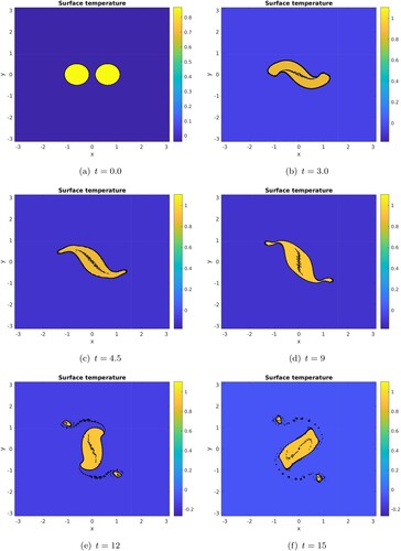
Out of the merged vortex, filaments of unit temperature also become unstable and form alleys of small vortices, followed by larger vortices, which have detached from the central vortex. Note that the appearance in figure 1 of smaller-scale vortices at the periphery of the core formed after the merger of two initially circular vortices is indicated in Sokolovskiy et al. (2018) as a characteristic feature of the merging process. It can also be seen that, at time t = 15.0, the merged vortex is still deformed by a complex vortex boundary perturbation (including an elliptical mode 2 and a square mode 4).

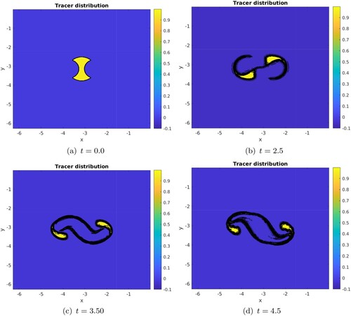
The Okubo-Weiss quantity OW, shown in figure 2, indicates a strong deformation along the central front and along the vortex boundary. The frontogenetic function clearly shows the tendency to intensify temperature gradients at the central front and at the tips of the merged vortex. The former corresponds to the transformation of the central front into a small vortex. The latter eventually leads to the formation of the external filaments, and of the small external vortices. To further investigate whether external fluid is trapped in the merged vortex core, we follow the evolution of passive tracer field during the interaction. We seed this tracer in a region bounded by a circle centred at the origin and by the vortices edge, see the top-left panel of figure 3. Clearly, the tracer patch is initially cut into two halves by the shear induced by the two-vortex flow. This patch is elongated and sheds filaments. It is most elongated where the Okubo-Weiss quantity OW is maximal, and a strong gradient forms along the merged vortex contour (as predicted by the frontogenetic function distribution). Two, non elongated, small patches resist shear at the tip of the vortex. Note that though tracer crosses the vortex core, it does not remain there. Therefore, the temperature intense front observed at the vortex centre does not correspond to some trapped external fluid, but to the initial vortex peripheries themselves.

Figure 2. Okubo-Weiss quantity OW (left panel) and frontogenetic function FGT map (right panel) in the $(x,y)$-plane at time t = 3 illustrating the deformation of the internal front for $d/R=2.5$ at resolution $1024\times 1024$. The black lines in the left hand panel are the contours of the various levels of the Okubo-Weiss parameter between 0 and the maximal positive or negative values. (a) OW – t = 3.0 and (b) FGT – t = 3.0 (Colour online).

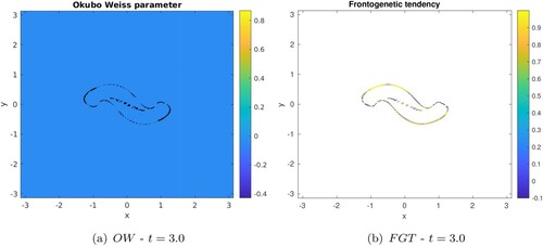
Figure 3. Evolution of the passive tracer distribution in the $(x,y)$-plane from left to right then top to bottom at time t = 0, 1.5, 3.0, 4.5 for $d/R=2.5$ at resolution $1024\times 1024$. The black lines denote the various levels of tracer concentration; their closeness indicates a locally strong tracer gradient. (a) t = 0.0. (b) t = 2.5. (c) t = 3.50 and (d) t = 4.5 (Colour online).

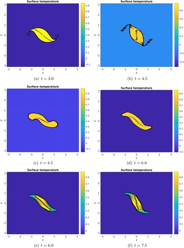
Once we have analysed the first steps of the merger process and of the formation of the internal front, we investigate how general this phenomenon is. To that purpose we show the evolution of two top-hat vortices initially separated by a distance d = 2R (figure 4, top row), or by a distance d = 2.8R (figure 4, middle row), and finally for two smooth vortices with $d=2.3R$. In all cases, the central front appears and breaks up into a row of filaments. The central front, the vortices, the filaments also form if a harmonic dissipation is used instead of a bi-harmonic operator. Therefore, this process is not related to a Gibbs like phenomenon (all the more so as the initial radial profiles of temperature have been slightly smoothed also for the top-hat vortices as mentioned in section 2). This process is physical and is observed for various initial radial profiles of temperature in each vortex, various initial vortex separations, and does not depend on the details of the dissipation.

Figure 4. Evolution of the temperature in the $(x,y)$-plane at time t = 3.0, 4.5 for top-hat vortices with $d/R=2.0$ (top row), at time t = 4.5, 6.0 for top-hat vortices with $d/R=2.8$ (middle row), at time t = 6.0, 7.5 for smooth vortices with $d/R=2.3$ (bottom row). These simulations were performed at $1024\times 1024$ resolution. The black lines are the contours of the various levels of temperature in the model. Their closeness indicates a high gradient of temperature. (a) t = 3.0. (b) t = 4.5. (c) t = 4.5. (d) t = 6.0. (e) t = 6.0 and (f) t = 7.5.

3.2. Instability of the central front

To understand the unstable evolution of the front in the core of the merged vortex, we next study the instability of a central temperature front in a parallel strip of constant temperature. This specific geometry (the parallel geometry) simplifies our problem further.

3.2.1. Linear stability analysis of a parallel temperature front in a strip

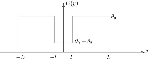
From the previous simulation, we observe that the central front is nearly parallel to the vortex boundary in the first stage of merger. This suggests to replace the quasi-elliptic vortex shape by a parallel strip of piecewise-constant temperature. Hence we consider here a meridionally symmetric temperature distribution as a basic state (see figure 5) (10) $\overline{\Theta }(y)=\{\begin{array}{lrl}{\theta }_0-{\theta }_2,& & |y|<l,\\ {\theta }_0,& l& <|y|<L,\\ 0,& L& <|y|,\end{array}$(10) and we study its linear stability. The zonal velocity induced by the strip is (11) $\overline{U}(y)=\frac{{\theta }_0}{\pi }\ln \left|\frac{y-L}{y+L}\right|-\frac{{\theta }_2}{\pi }\ln \left|\frac{y-l}{y+l}\right|,$(11) which has a singularity at the temperature fronts.

Figure 5. Meridional section of the temperature distribution in the parallel strip under study.

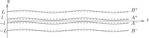
We follow Juckes (1995) and Harvey and Ambaum (2010) for the derivation of the linear stability analysis. Thus, to assess the stability of this temperature and velocity distribution, we perturb initially the above temperature profile by displacing the temperature fronts at $y=\pm l$ and $y=\pm L$ (see figure 6): (12) $\pm l\to \pm l+\epsilon A^{\pm }(t)\exp (\mathrm{i}kx),\pm L\to \pm L+\epsilon B^{\pm }(t)\exp (\mathrm{i}kx).$(12) Assuming that $\epsilon \ll 1$, the surface temperature perturbation is (13) ${\Theta }^{\prime }(x,y,t)=\epsilon \exp (\mathrm{i}kx)[B^{-}{\theta }_0\delta (-L)-A^{-}{\theta }_2\delta (-l)+A^{+}{\theta }_2\delta (l)-B^{+}{\theta }_0\delta (L)],$(13) where $\delta (x)$ is the Dirac distribution at x, and we determine the corresponding streamfunction perturbation which evolves in time as (14) $\begin{array}{rl}{\psi }^{\prime }(x,y,t)& =\epsilon \exp (\mathrm{i}kx)[\frac{{\theta }_0}{\pi }[B^{-}{\mathrm{K}}_0(k|y+L|)-B^{+}{\mathrm{K}}_0(k|y-L|)]\\ & -\frac{{\theta }_2}{\pi }[A^{-}{\mathrm{K}}_0(k|y+l|)-A^{+}{\mathrm{K}}_0(k|y-l|)]],\end{array}$(14) where ${\mathrm{K}}_0(x)$ is the modified Bessel function of the second kind and of zeroth order. Furthermore, we set $U_0^{\ast }={\theta }_0/\pi$ and $U_2^{\ast }={\theta }_2/\pi$. Considering the perturbation at $\eta =\hat{\eta }\exp (\mathrm{i}k(x-ct))$, the stability problem can be addressed using exponentially growing normal modes (15) $\begin{array}{r}{\displaystyle \frac{\mathrm{d}B}{\mathrm{d}t}}={\displaystyle \frac{\mathrm{\partial }\eta }{\mathrm{\partial }t}}+\overline{U}(y){\displaystyle \frac{\mathrm{\partial }\eta }{\mathrm{\partial }x}}=-\mathrm{i}k\overline{U}(y)-c)\hat{\eta }=\mathrm{i}k{\psi }^{\prime },\end{array}$(15) (16) $\begin{array}{r}c\hat{\eta }=[\overline{U}(y)\hat{\eta }-{\psi }^{\prime }].\end{array}$(16) At $y=-L+ϵB^{-}\exp (\mathrm{i}kx)$, we have (17) $\begin{array}{rl}c{B}^{-}& =\underset{y\to -L}{lim}[\overline{U}{B}^{-}-{\psi }^{\prime }],\end{array}$(17) (18) $\begin{array}{rl}c{B}^{-}& =B^{-}{U}_0^{\ast }\underset{y\to -L}{lim}[-\ln |k(y+L)/2|-{\mathrm{K}}_0(k|y+L|)]\\ & +B^{-}[U_0^{\ast }\ln |kL|+U_2^{\ast }\ln |k(L-l)|-U_2^{\ast }\ln |k(L+l)|]\\ & +A^{-}{U}_2^{\ast }{\mathrm{K}}_0(k|L-l|)-A^{+}{U}_2^{\ast }{\mathrm{K}}_0(k|L+l|)+B^{+}{U}_0^{\ast }{\mathrm{K}}_0(2kL),\end{array}$(18) (19) $\begin{array}{rl}c{B}^{-}& =B^{-}[U_0^{\ast }(\gamma +\ln |kL|)+U_2^{\ast }\ln |k(L-l)|-U_2^{\ast }\ln |k(L+l)|]\\ & +A^{-}{U}_2^{\ast }{\mathrm{K}}_0(k|L-l|)-A^{+}{U}_2^{\ast }{\mathrm{K}}_0(k|L+l|)+B^{+}{U}_0^{\ast }{\mathrm{K}}_0(2kL),\end{array}$(19) where γ is Euler's constant, obtained through the relation ${\mathrm{K}}_0(x)\simeq -\ln (x/2)-\gamma$, for small x (Abramovitch & Stegun, 9.6.13, page 375). Similarly, we have:

• at $y=-l+A^{-}\exp (\mathrm{i}kx)$, (20) $\begin{array}{rl}c{A}^{-}& =A^{-}[U_2^{\ast }(-\gamma -\ln |kl|)+U_0^{\ast }\ln |k(L+l)|-U_0^{\ast }\ln |k(L-l)|]\\ & -A^{+}{U}_2^{\ast }{\mathrm{K}}_0(2kl)-B^{-}{U}_0^{\ast }{\mathrm{K}}_0(k|L-l|)+B^{+}{U}_0^{\ast }{\mathrm{K}}_0(k|L+l|);\end{array}$(20)

• at $y=l+A^{+}\exp (\mathrm{i}kx)$, (21) $\begin{array}{rl}c{A}^{+}& =A^{+}[U_2^{\ast }(\gamma +\ln |kl|)+U_0^{\ast }\ln |k(L-l)|-U_0^{\ast }\ln |k(L+l)|]\\ & +A^{-}{U}_2^{\ast }{\mathrm{K}}_0(2kl)-B^{-}{U}_0^{\ast }{\mathrm{K}}_0(k|L+l|)+B^{+}{U}_0^{\ast }{\mathrm{K}}_0(k|L-l|);\end{array}$(21)

• at $y=L+B^{+}\exp (\mathrm{i}kx)$, (22) $\begin{array}{rl}c{B}^{+}& =B^{+}[U_0^{\ast }(-\gamma -\ln |kL|)+U_2^{\ast }\ln |k(L+l)|-U_2^{\ast }\ln |k(L-l)|]\\ & +A^{-}{U}_2^{\ast }{\mathrm{K}}_0(k|L+l|)-A^{+}{U}_2^{\ast }{\mathrm{K}}_0(k|L-l|)-B^{-}{U}_0^{\ast }{\mathrm{K}}_0(2kL).\end{array}$(22)

Figure 6. Horizontal structure of the temperature distribution in the perturbed parallel gaped strip.

This set of equations may be expressed in matrix form (23) $c[B^{-},A^{-},A^{+},B^{+}{]}^{\mathsf{T}}=\mathsf{M}[B^{-},A^{-},A^{+},B^{+}{]}^{\mathsf{T}}$(23) where the superscript $\mathsf{T}$ denotes the transpose, and (24) $\mathsf{M}=\left[\begin{array}{cccc}{P}_1& U_2^{\ast }{\mathrm{K}}_0(k|L-l|)& -U_2^{\ast }{\mathrm{K}}_0(k|L+l|)& U_0^{\ast }{\mathrm{K}}_0(2kL)\\ -U_0^{\ast }{\mathrm{K}}_0(k|L-l|)& -P_2& -U_2^{\ast }{\mathrm{K}}_0(2kl)& U_0^{\ast }{\mathrm{K}}_0(k|L+l|)\\ -U_0^{\ast }{\mathrm{K}}_0(k|L+l|)& U_2^{\ast }{\mathrm{K}}_0(2kl)& P_2& U_0^{\ast }{\mathrm{K}}_0(k|L-l|)\\ -U_0^{\ast }{\mathrm{K}}_0(2kL)& U_2^{\ast }{\mathrm{K}}_0(k|L+l|)& -U_2^{\ast }{\mathrm{K}}_0(k|L-l|)& -P_1\end{array}\right],$(24) in which (25) $\begin{array}{rl}{P}_1& =U_0^{\ast }(\gamma +\ln |kL|)+U_2^{\ast }\ln |k(L-l)|-U_2^{\ast }\ln |k(L+l)|,\end{array}$(25) (26) $\begin{array}{rl}{P}_2& =U_2^{\ast }(\gamma +\ln |kl|)+U_0^{\ast }\ln |k(L-l)|-U_0^{\ast }\ln |k(L+l)|.\end{array}$(26) This results in a eigenvalue problem, where the eigenvalues are the modes' complex speed σ and the eigenvectors are the modes complex amplitudes $[B^{-},A^{-},A^{+},B^{+}{]}^{\mathsf{T}}$. Results are reported in figure 7 for the growth rate $\sigma =-k\mathrm{Im}\{c\}$, where $\mathrm{Im}\{\}$ stands for the imaginary part.

Figure 7. Growth rates of linear perturbation on the mean temperature profile; the growth rates are displayed in the $(kL,l/L)$-plane for $U_2^{\ast }/U_0^{\ast }=0.1,0.5,0.9$ (left column) and in the (kL, $U_2^{\ast }/U_0^{\ast }$)-plane for $l/L=0.1,0.5,0.9$ (right column).

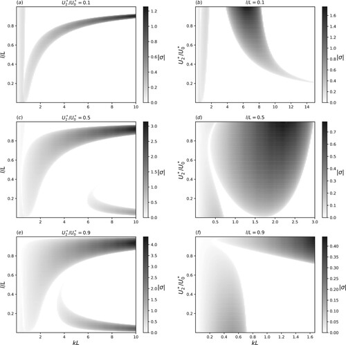
In the first column of figure 7, long waves are unstable for small $U_2^{\ast }/U_0^{\ast }$. The range of unstable wavenumbers widens when increasing $U_2^{\ast }/U_0^{\ast }$. Thus increasing the shear (the temperature jumps over the filament) makes the flow more unstable because of the stronger interaction between internal and external fronts. If these fronts get closer (increasing l/L), this instability also strengthens. For a large shear, a third band of growth rate appears for a small inner gap at high wavenumbers, and for smaller wavenumbers as $U_2^{\ast }/U_0^{\ast }$ increases. This is the signature of the interaction of internal fronts. Indeed, as l/L increases, this instability gets reduced as both fronts get spatially separated.

For the second column, the observed range of kL for instability depends on the width of the inner gap $2l$ compared to the overall width of the filament $2L$. For increasing l/L, unstable waves is associated with low wavenumbers.

For $l/L=0.1$, a third band of growth rates is found for short wavenumbers; this reveals that increasing the shear enhances the instability due to the interaction of both internal fronts. For high wavelengths (low kL), instability occurs for all shears. Two regions of instability may be observed, and they extend up to larger wavenumbers as the inner gap widens. This relates to the external front getting closer to the inner one and therefore interacting with it.

3.2.2. Nonlinear evolution of the unstable parallel flow

We next numerically model the nonlinear evolution of a perturbed parallel (meridionally symmetric) strip of temperature with a central gap. This strip is initially perturbed with a weak amplitude, white noise, temperature distribution. The same spectral code as in section 2.1, is used. We set $U_0^{\ast }=1,L=1$.

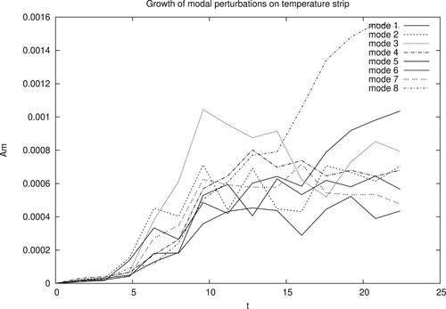
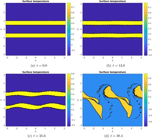
Figure 8 shows a time sequence of surface temperature maps. As indicated by the linear stability analysis, a short wave pattern (wavenumber m = 8) forms. We also note that longer waves develop from the short waves on the central temperature strip. The outer boundary remains fairly flat. Once the inner perturbations have grown to finite amplitude, they occlude as elliptical vortices. These central vortices then merge by pairs. This merging process also leads to filamentation and these long filaments, which lie between the merged vortices, roll up into vortices themselves. Even more interesting, as shown by the last subplot of figure 8, the central vortex in the line, has also trapped a front or a filament which has formed smaller vortices in its core. Therefore this vortex-in-core process appears as multi-scale. We have not simulated the evolution of temperature strips with small values of δ which should be close to those studied by Juckes (1995). Figure 9 shows the modal analysis of the previous simulation. All waves grow, with two notable predominances: medium waves (m = 3) at intermediate time (5<t<12) and short waves (m = 8) at later time (t>15). The final co-existence of multiple waves reflects the rather turbulent state at the strip centre, including the small vortices but also filaments of temperature. It also reflects (since this is a zonal modal analysis) the fact that the perturbations do not remain zonally aligned at all times. We detail two further cases with $U_2^{\ast }/U_0^{\ast }=1.0$, one with $l/L=0.5$ and one with $l/L=0.9$ in appendix (see figures A1 and A2).

Figure 8. Nonlinear evolution of the unstable parallel temperature distribution with $l/L=0.1,U_2^{\ast }/U_0^{\ast }=1.0$, perturbed with a white noise in temperature with amplitude 0.1 initially, at time t = 0, 8.0, 16.0, 20.0, 24.0 (from left to right and from top to bottom). The lower left plot is a zoom on the central vortex for the last subplot. These simulations were performed at $1024\times 1024$ resolution. The black lines are the various contours of temperature. Their closeness denotes a high gradient of temperature, in particular in the filaments. (a) t = 0.1. (b) t = 8.0. (c) t = 16.0. (d) t = 20.0. (e) t = 24.0 and (f) t = 24.0 – zoom.

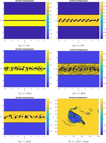
Figure 9. Modal analysis ($A_m$ is the amplitude of the zonal mode with wavenumber m) for the unstable parallel temperature distribution with $l/L=0.1,U_2^{\ast }/U_0^{\ast }=1.0$ presented in figure 8.

3.3. Formation and further evolution of the small vortices in the core of the merged vortex

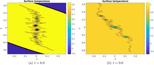
Following this intermediate study on the stability of a central strip, we revisit our initial example of the merger of two top-hat vortices initially separated by a distance d = 2.5R (see figure 1). We have observed that a central strip of anomalous temperature in a uniform temperature environment is prone to barotropic (horizontal shear) instability, all the stronger as this strip is narrower. Figure 10 clearly shows that a row of small vortices has formed from the shear instability of the central strip (t = 6) and that a secondary instability ensues in which the small vortices merge and former longer, more elliptical vortices in the core of the large vortex.

Figure 10. Zoom on the central region of figure 1 at time t = 6.0 and t = 9.0; row of small vortices in the core of the large merged vortex. The black lines indicate the various levels of surface temperature, separating the various colours. (a) t = 6.0 and (b) t = 9.0 (Colour online).

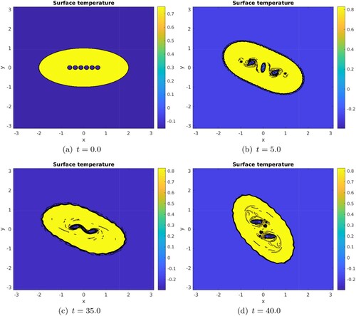
Since we cannot control the internal arrangement of the small vortices in the large merged vortex, from the initial conditions of the two vortices only, we next initialise a row of small vortices inside a large elliptical vortex, and we study their evolution. This situation mimics the elliptical vortex state of our first simulation (figure 1). We initialise an ellipse with a 2:1 ratio of major to minor axes (a = 2, b = 1), close to that of the vortex at t = 12 in this initial simulation. We arrange a row of 6 small vortices, regularly aligned and centred along the major axis. These vortices have radius $R_1$ and are separated by a distance $d^{\prime }$ along the major axis. We ran 3 simulations, respectively with $R_1=0.05,d^{\prime }=0.25$, $R_1=0.1,d^{\prime }=0.25$, $R_1=0.1,d^{\prime }=0.2$. In the first case (not shown), the two central small vortices merge and for the rest of the simulation (until t = 100), the five vortices form a configuration oscillating between a straight line and a S-shaped structure; therefore this 5-vortex structure is robust. In the second case presented in figure 11, the 6 vortices rapidly evolve, via three mergers, to a 3-vortex configuration, which later undergoes a bifurcation to a 2-vortex configuration. This bifurcation occurs via the connection of the three vortices near the centre. The central vortex forms a “bridge” between the two outer ones. These two vortices each absorb part of the central vortex (see times t = 35, 40). At time t = 100 the two small vortices are still present along the major axis, and they are themselves elliptical (not shown). In the third case (not shown) the transition from 6 to 2 small vortices results from the single merger (it does not imply an intermediate 3-vortex state). These two vortices then interact periodically as they near the centre of the large vortex. These partial and temporary interactions are followed by stages of parting of the two vortices along the major axis and the cycle repeats. It must be noted that, in the last stage of the evolution, an asymmetry starts to grow in this central configuration.

Figure 11. Time evolution of horizontal maps of temperature using the nonlinear spectral SQG model. Times shown are t = 0, 5, 35, 40. The simulation is initialised with 6 small vortices along the major axis of a 2:1 large elliptical vortex. The small vortices have the following radius and separation $R_1=0.1,d^{\prime }=0.25$. This simulation was performed at $1024\times 1024$ resolution. The black lines indicate the various contours of temperature. The temperature gradients are large in the filaments and at the vortex peripheries. (a) t = 0.0. (b) t = 5.0. (c) t = 35.0 and (d) t = 40.0 (Colour online).

We have calculated the shear and strain field inside an elliptical temperature vortex in the absence of the small vortices. For this elliptical vortex, we have chosen two temperature distributions: one top-hat and one which is the square-root of a parabolic profile (Dritschel 2010). For the top-hat profile, the shear and strain are concentrated at the edge of the ellipse due to the velocity discontinuity there. For the parabolic profile (figure not shown), there is no velocity discontinuity at the edge of the ellipse; the shear and strain are intense there, but the shear is also intense along the main axis of the ellipse. That is where the small vortices lie in our simulations. Therefore these small vortices interact mutually under the influence of a larger-scale strain and rotation flow. Previous work (Perrot and Carton 2009, 2010, Vic et al. 2021) has shown that the presence of a large-scale shear and rotation flow renders the trajectory of two vortices complex and that their merger is favoured or hindered depending on their orientation with respect to the direction of the shear. Clearly, here, the small vortices which are close together do not merge and this may be attributed to the presence of the large-scale deformation flow.

4. Discussion and conclusion

Motivated by the close examination of the merger of two circular vortices in a high-resolution SQG simulation (Carton et al. 2016, Ciani et al. 2016), we have run very high-resolution simulations of this process with very low viscosity, and we have determined that a temperature front is trapped and forms a strip in the core of the large merged vortex. This front breaks into small vortices which can later interact, forming filaments and slightly larger vortices in the core of the large vortex. We have shown that this process is not dependent on the initial distance between the two circular vortices, nor on their radial temperature profile (top-hat), nor on the type of viscosity used (harmonic or biharmonic). It can be noted that similar simulations were performed using a semi-Lagrangian code (Combined Lagrangian Advection Method developed by Dritschel and Fontane 2010) which produced the same evolution (not shown).

We analysed the evolution of the vortices during merger using diagnostics of

• the passive tracer evolution which showed that little fluid initially between the two circular vortices ends up in the core of the merged vortex,

• the Okubo-Weiss quantity which showed that strong deformation occurred at the merged vortex edge but also in its core,

• the frontogenetic function which highlighted the intensification of the internal front.

To better understand the instability of the central front, we designed a few experiments evaluating the instability of a gapped parallel strip of temperature. We calculated the linear instability and showed that, for a narrow gap, small vortices form at the centre of the strip. We analysed this simulation in terms of longitudinal wavelengths.

Finally, to better understand the last stage in the evolution of the merged vortex (the evolution of the small vortices in the final elliptical vortex), we designed a few experiments using an elliptical temperature patch, with small inner vortices. Their evolutions favourably compared with that of the merged vortex.

Obviously, these simulations did not cover all types of vortices, every possible initial states, nor covered all values of the physical parameters (numerical dissipation in particular), and they remain idealised compared to actual oceanic observations. Zhang and McGillicuddy (2020) describe an intrusion of external fluid into and over a Gulf Stream Ring, and the formation of a warm spiral vortex. This process is essentially due to a horizontal advection as in our study. But other, baroclinic effects can also lead to the formation of small vortices in the core of larger ones: Brannigan et al. (2017) describes submesoscale features in the core of a Gulf Stream ring, originating from ageostrophic instability. Legg et al. (1998) presents evidence of the formation of small convective cyclones in the core of mesoscale vortices. In fact, the small vortices formed in our experiments have a shallow vertical extent ($h=f_{0}R/N_0$) whereas convectively formed vortices are deep reaching, and can easily be identified as such. These previous studies showed that, when small eddies are formed by baroclinic processes in the core of larger vortices, they can lead to vertical mixing. Therefore, the question arises here as to the importance of the small vortices in fluid mixing in the core of the larger vortex. To address this question, we run two very high-resolution simulations of the SQG model, for vortices with or without a passive tracer. In the first experiment (shown on figure 12), we initialised an elliptical vortex containing positive tracer (Tr = +1) on the right-hand side, and negative tracer (Tr = −1) on the left-hand side. In the second experiment (same figure, bottom row), the same distribution was used and small vortices with null temperature and null tracer were added along the major axis of the ellipse (6 vortices with radius R = 0.1 separated by a distance $d^{\prime }=0.25$).

Figure 12. Evolution of horizontal maps of passive tracer for an ellipse without (top) or with (bottom) small central vortices. Times shown are t = 0, 16, 32. The second simulation is initialised with 6 small vortices along the major axis of a 2:1 large elliptical vortex. The small vortices have the following radius and separation $R_1=0.1,d=0.25$. The resolution of this simulation is $1024\times 1024$. The black lines indicate the various levels of tracer concentration. (a) t = 0.0. (b) t = 16.0. (c) t = 32.0. (d) t = 0.0. (e) t = 16.0 and (f) t = 32.0 (Colour online).

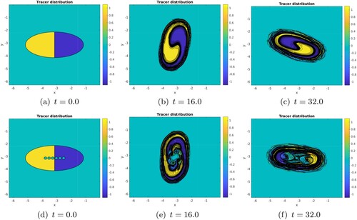
Clearly, in the first case, the tracers are stirred by differential advection and form a spiral pattern inside the ellipse. Stirring and entrainment occurs at the vortex periphery where more mixing is observed. In the second case, the irregular and multi-scale dynamics induced by the small vortices lead to a downscale tracer flux, in particular in the presence of sheared regions such as filaments. Therefore these small-scale dynamics favour the mixing and homogenisation of tracers (e.g. chemical elements or biological species) in a region considered as isolated from the external ocean.

Finally, a natural extension of this study would proceed via the use of a 3D primitive equation model which would allow the development of cyclone/anticyclone asymmetry, of stronger vertical velocities, and the presence of ageostrophic instabilities. The role of an external deformation flow, particularly in the mixing of tracer, should also be investigated. It can also be noted that the same small scale inner vortices were observed during the merger of two like-signed vortices in a three-vortex collapse interaction in Reinaud et al. (2022) in generalised Euler's equations, indicating that this may be a common occurrence in vortex merger even under other mathematical models.

Acknowledgments

We thank LOPS and UBO for a M.Sc internship grant which allowed the first author to carry out this work

Disclosure statement

No potential conflict of interest was reported by the author(s).

Appendix: Evolution of unstable parallel temperature distributions

In this appendix, we show the evolution of two other unstable parallel temperature distributions. They have respectively $\mu =0.5$ and $\mu =0.9$ both with $\delta =1.0$. In the first case (see figure A1, the null temperature strip width is half the distance between the two strips. so that the instability develops under the influence of the interaction between the strips. The small-scale perturbations grow initially and then give birth to longer scale perturbations. The two strips break up into two vortices which finally interact (see the last plot of this figure). Again, this interactions leads to the formation of filaments and of small vortices.

Figure A1. Nonlinear evolution of the unstable parallel temperature distribution with $l/L=0.5,U_2^{\ast }/U_0^{\ast }=1.0$, perturbed with a white noise in temperature with amplitude 0.1 initially, at time t = 0, 12.8, 25.6, 38.4. The black lines indicate the various levels of surface temperature. (a) t = 0.0. (b) t = 12.8. (c) t = 25.6 and (d) t = 38.4 (Colour online).

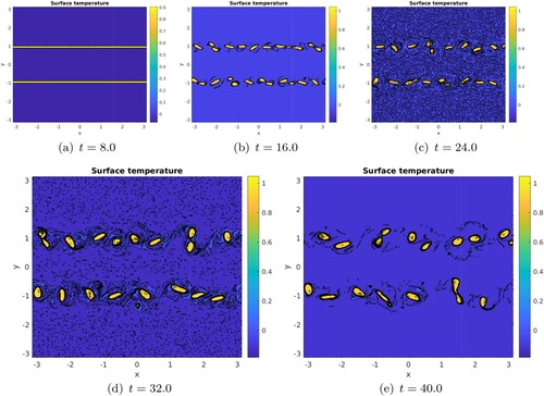
The second case has narrow external (well separated) strips of unit temperature (see figure A2). Since the shear is stronger here than in the previous case, the unstable evolution is faster and the temperature strips breaks up as a vortex row. A secondary instability occurs by which the vortices in the same strip, merge. These mergers are followed by other vortex interactions which produce filaments and small vortices.

Figure A2. Nonlinear evolution of the unstable parallel temperature distribution with $l/L=0.9,U_2^{\ast }/U_0^{\ast }=1.0$, perturbed with a white noise in temperature with amplitude 0.1 initially, at time t = 0, 8.0, 16.0, 24.0, 32.0, 40.0. The black lines indicate the various levels of surface temperature. (a) t = 8.0. (b) t = 16.0. (c) t = 24.0. (d) t = 32.0 and (e) t = 40.0 (Colour online).

References

- Bambrey, R.R., Reinaud, J.N. and Dritschel, D.G., Strong interactions between two co-rotating quasi-geostrophic vortices. J. Fluid Mech. 2007, 592, 117–133.
- Brandt, L.K. and Nomura, K.K., The physics of vortex merger: further insight. Phys. Fluids 2006, 18, Article ID 051701.
- Brannigan, L., Marshall, D.P., Naveira Garabato, A.C., Nurser, A.J.G. and Kaiser, J., Submesoscale instabilities in mesoscale eddies. J. Phys. Oceanogr. 2017, 47, 3061–3085.
- Capéran, P. and Verron, J., Numerical simulation of a physical experiment on two-dimensional vortex merger. Fluid Dyn. Res. 1988, 3, 87–92.
- Carton, X., On the merger of shielded vortices. Europhys. Lett. 1992, 18, 697–703.
- Carton, X., Ciani, D., Verron, J., Reinaud, J.N. and Sokolovskiy, M.A., Vortex merger in surface quasi-geostrophy. Geophys. Astrophys. Fluid Dyn. 2016, 110, 1–22.
- Carton, X., Morvan, M., Reinaud, J.N., Sokolovskiy, M.A., L'Hégaret, P. and Vic, C., Vortex merger near a topographic slope in a homogeneous rotating fluid. Reg. Chaotic Dyn. 2017, 22, 455–478.
- Ciani, D., Carton, X. and Verron, J., On the merger of subsurface isolated vortices. Geophys. Astrophys. Fluid Dyn. 2016, 110, 23–49.
- Cresswell, G.R., The coalescence of two East Australian warm-core eddies. Science 1982, 215, 161–164.
- Dritschel, D.G., Vortex merger in rotating stratified flows. J. Fluid Mech. 2002, 455, 83–101.
- Dritschel, D.G., An exact steadily rotating surface quasi-geostrophic elliptical vortex. Geophys. Astrophys. Fluid Dyn. 2010, 105, 368–376.
- Dritschel, D.G. and Fontane, J., The combined Lagrangian advection method. J. Comput. Phys. 2010, 229, 5408–5417.
- Harvey, B.J. and Ambaum, M.H.P., Instability of surface-temperature filaments in strain and shear. Quart. J. Royal Met. Soc. 2010, 136, 1509–1513.
- Held, I.M., Pierrehumbert, R.T., Garner, S.T. and Swanson, K.L., Surface quasi-geostrophic dynamics.. J. Fluid Mech. 1995, 282, 1–20.
- Hopfinger, E.J. and van Heijst, G.J.F., Vortices in rotating fluids. Ann. Rev. Fluid Mech. 1993, 25, 241–289.
- Juckes, M., Instability of surface and upper-tropospheric shear lines. J. Atmos. Sci. 1995, 52, 3247–3252.
- Legg, S., McWilliams, J.C. and Gao, J., Localization of deep ocean convection by a mesoscale eddy.. J. Phys. Oceanogr. 1998, 28, 944–970.
- Legras, B. and Dritschel, D.G., The erosion of a distributed two-dimensional vortex in a background straining flow. J. Fluid Mech. 2001, 441, 369–398.
- Melander, M.V., Zabusky, N. and McWilliams, J.C., Symmetric vortex merger in two dimensions: causes and conditions. J. Fluid Mech. 1988, 195, 303–340.
- Morvan, M., L'Hegaret, P., Carton, X., Gula, J., Vic, C., de Marez, C., Sokolovskiy, M. and Koshel, K., The life cycle of submesoscale eddies generated by topographic interactions. Ocean Sci. 2019, 15, 1531–1543.
- Okubo, A., Horizontal dispersion of floatable particles in the vicinity of velocity singularities such as convergences. Deep-Sea Res. 1970, 17, 445–454.
- Overman II, E.A. and Zabusky, N.J., Evolution and merger of isolated vortex structures. Phys. Fluids 1982, 25, 1297–1305.
- Ozugurlu, E., Reinaud, J.N. and Dritschel, D.G., Interaction between two quasi-geostrophic vortices of unequal potential-vorticity. J. Fluid Mech. 2008, 597, 395–414.
- Pavia, E.G. and Cushman-Roisin, B., Merging of frontal eddies. J. Phys. Oceanogr. 1990, 20, 1886–1906.
- Perrot, X. and Carton, X., Point-vortex interaction in an oscillatory deformation field: Hamiltonian dynamics, harmonic resonance and transition to chaos. Discr. Cont. Dyn. Syst. B 2009, 11, 971–995.
- Perrot, X. and Carton, X., 2D vortex interaction in a non uniform flow. Theor. Comput. Fluid Dyn. 2010, 24, 95–100.
- Reinaud, J.N. and Dritschel, D.G., The merger of vertically offset quasi-geostrophic vortices. J. Fluid Mech. 2002, 469, 297–315.
- Reinaud, J.N. and Dritschel, D.G., The critical merger distance between two co-rotating quasi-geostrophic vortices. J. Fluid Mech. 2005, 522, 357–381.
- Reinaud, J.N. and Dritschel, D.G., The merger of geophysical vortices at finite Rossby and Froude number. J. Fluid Mech. 2019, 848, 388–410.
- Reinaud, J.N., Dritschel, D.G. and Scott, R.K., Self-similar collapse of three vortices in the generalised Euler and quasi-geostrophic equations. Physica D 2022, 434, Article ID 133226.
- Saffman, P.G. and Szeto, R., Equilibrium shapes of a pair of equal uniform vortices. Phys. Fluids 1980, 23, 2338–2342.
- Sokolovskiy, M.A. and Verron, J., Finite-core hetons: stability and interactions. J. Fluid Mech. 2000, 423, 127–154.
- Sokolovskiy, M.A. and Verron, J., Vortex Structures in a Stratified Rotating Fluid, Vol. 47, Atmos. Oceanogr. Sci. Lib 2014 (Springer: Cham/Heidelberg/New York/Dordrecht/London).
- Sokolovskiy, M.A., Verron, J. and Carton, X.J., The formation of new quasi-stationary vortex patterns from the interaction of two identical vortices in a rotating fluid. Ocean Dyn. 2018, 68, 723–733.
- Valcke, S. and Verron, J., On interactions between two finite-core hetons. Phys. Fluids 1993, A5, 2058–2060.
- Valcke, S. and Verron, J., Cyclone-anticyclone asymmetry in the merging process. Dyn. Atmos. Oceans 1996, 24, 227–236.
- Valcke, S. and Verron, J., Interactions of baroclinic isolated vortices: the dominant effect of shielding. J. Phys. Oceanogr. 1997, 27, 524–541.
- Verron, J. and Hopfinger, E., The enigmatic merging conditions of two-layer baroclinic vortices. C.R. Acad. Sci. Paris, Ser. II 1991, 313, 737–742.
- Verron, J. and Valcke, S., Scale-dependent merging of baroclinic vortices. J. Fluid Mech. 1994, 264, 81–106.
- Verron, J., Hopfinger, E. and McWilliams, J.C., Sensitivity to initial conditions in the merging of two-layer baroclinic vortices. Phys. Fluids 1990, A2, 886–889.
- Vic, A., Carton, X. and Gula, J., The interaction of two unsteady point vortex sources in a deformation field in 2D incompressible flows. Regul. Chaot. Dyn 2021, 26, 618–646.
- von Hardenberg, J., McWilliams, J.C., Provenzale, A., Shchpetkin, A. and Weiss, J.B., Vortex merging in quasi-geostrohic flows. J. Fluid Mech. 2000, 412, 331–353.
- Weiss, J., The dynamics of enstrophy transfer in two-dimensional hydrodynamics. Physica D 1991, 48, 273–294.
- Zhang, W. and McGillicuddy, D.J.J., Warm spiral streamers over gulf stream Warm-Core rings. J. Phys. Oceanogr. 2020, 50, 3331–3351.
- Zhang, Z., Wang, W. and Qiu, B., Oceanic mass transport by mesoscale eddies. Science 2014, 345, 322–324.