Exploring regional wage dispersion in Swedish manufacturing, 1860–2009

ABSTRACT

Economic theory predicts that regional wages will converge as transport and communication technologies bring labour markets together. An exploration of this transition from labour market segmentation to unification requires long-term evidence of nominal wages and cost of living by region. This paper presents new evidence of wages for male manufacturing workers and cost-of-living indices across 24 Swedish counties between 1860 and 2009. Our findings indicate that the Swedish regional wage differentials were a great deal larger in the 1860s than in the 2000s. Most of the compression took place between the 1860s and World War I, as well as in the 1930s and during World War II. Differences in expenditures on housing impact on our assessment of convergence in the post-World War II decades: the nominal measure declines, while the real one stays constant. Our concluding discussion engages with the assumption that before World War I, regional wage convergence was associated with labour mobility, spurred by improved communication and transportation technologies as well as by the implementation of modern employment contracts. In the 1930s and 1940s, in contrast, regional wage convergence can be traced to high unionisation and centralised collective bargaining in the labour market, two distinguishing features of the Swedish Model.

KEYWORDS:

• Regional wage convergence
• regional cost of living
• labour market institutions
• labour mobility
• labour market integration

JEL CODES:

• N93
• N94

1. Introduction

The assumption that the labour market is subjected to the same forces of supply and demand that act upon the goods market goes back to Marshall (1920, book 6, Ch. 3) and Hicks (1932, Ch. 4). Some authors go so far as to suggest that the law of one price, attributed to Cournot (1838/1971) and frequently mentioned in research on price convergence of goods (Federico, 2012), is also a useful metaphor for the labour market (Caruana Galizia, 2015; Rosenbloom, 1998, 2002).

The empirical implication of the law of one price in a labour market context is that wages will converge across space as improvements in transports and communications expand the geographical extent of labour markets. In the absence of migration barriers, migration from low-wage regions to high-wage regions tends to decrease regional wage differentials. Hence, wage convergence and co-movement of regional wages are signs of labour market integration.¹ Wage convergence, so the argument goes, will continue until workers equipped with the same human capital receive equal wages regardless of location, and notwithstanding site-specific attributes that may thwart equalisation in its entirety.² If wage differentials do decline as a result of modern economic growth, as the theory of integration postulates, then labour market integration is arguably one of the most important aspects of the entire modernisation process, and it also has a bearing on the evolution of inequality. Hence, this is a topic worthy of sustained and undivided attention.

The focus of this paper lies on the long-run behaviour of regional wages in Sweden. A growing body of research has examined the behaviour of regional wages in an historical context and shown that labour markets separated geographically have exhibited significant regional variations in wages.³ Some of the studies have found instances of wage convergence during the late nineteenth and early twentieth century and in the post-World War II era. It is, however, difficult to gain generic insights from these studies and thereby arrive at an adequate understanding of labour market integration because of disparities in the empirical strategies employed. Such disparities concern, for instance, worker characteristics and regional units. Some studies look into farm labour, while others look into construction and/or manufacturing workers. The regional units are not commensurable by size and administrative function: the wage data compiled for Sweden, a small country, refer to 24 counties, whereas studies of the American wage convergence usually split the country into 7 regions. Besides, wages are sometimes measured on an hourly basis, sometimes on an annual or daily basis. Yet another problem emerges in relation to the periods under consideration: these vary greatly, and most studies establish a period that is too short to allow us any systematic examination of long-run convergence. Finally, few studies control for the effect of regional cost-of-living indices, a procedure that can have a significant impact on the pattern of regional wage dispersion.

Our empirical strategy is devised to deal with the difficulties that stem from the methodological and data heterogeneity and to uncover the interactions of the short-term and the-long term behaviour of wage dispersion. Most of the heterogeneity-related issues have been eliminated by our focus on wage dispersion for male manufacturing workers throughout the entire period, excluding all salary employees.⁴ We have examined wage dispersion across 24 Swedish counties (län) between 1860 and 2009. This considerable time span made it possible to explore both the long-run development of regional wage differences and the impact of short-run disturbances on wage convergence.⁵ Our wage evidence originates from the published official statistics and from the original returns underlying public investigations and official statistics gathered in archives (see Appendix 1, Supplementary material for details). We have accounted for the effect of regional prices in foodstuff and housing rent by constructing 24 different cost-of-living indices (see Appendix 2, Supplementary material for details). House prices have been discarded, since they would inevitably have led to an overestimation of cost-of-living differentials. Increasing house prices entail increasing wealth; wealth and cost of living are distinct issues that should not be conflated. We have assessed the magnitude of real and nominal wage convergence by applying the two conventional tests for cross-sectional data (Barro & Sala-i-Martin, 1991): σ-convergence and unconditional and conditional β-convergence.

Our findings indicate that the Swedish regional wage differentials were a great deal larger in the 1860s than in the 2000s. Integration is indeed one of the major transformations that have taken place in the labour market since the mid-nineteenth century. The compression of these differentials did not occur continuously, but in brief intervals, which thus underlines the importance of examining both the short-run and the long-run behaviour of wage convergence. Compression took place between the 1860s and World War I, and in the 1930s and during World War II. Our assessment of wage convergence depends, to some extent, on cost-of-living differentials; the nominal measure declines from the 1960s onwards, whereas the real measure remains constant owing to differences in housing expenditures. This particular finding reinforces the importance of constructing regional cost-of-living indices (Coelho & Shepherd, 1974; Hatton & Williamson, 1991, 1993). Our concluding discussion, which breaks down the entire era into four sub-periods, brings the historical context to bear on our empirical results. Our concluding discussion engages with the assumption that before World War I, regional wage convergence occurred in tandem with labour mobility, facilitated by improved communication and transportation technologies as well as by the implementation of modern employment contracts. In the 1930s and 1940s, in contrast, regional wage convergence can be traced to high unionisation and centralised collective bargaining in the labour market, two distinguishing features of the Swedish Model.

2. Wages and cost of living by county

The following digression describes in broad strokes the most important aspects of the empirical foundation of this study. Details are provided in Appendices 1 and 2, Supplementary material; the data are presented in an online spreadsheet. The digression proceeds stepwise and begins with regional nominal wages.

The first step aimed at establishing a geographical classification of wages that was consistent over time: we chose the average wage per hour for male workers in manufacturing in 24 Swedish counties. The counties correspond to level 3 of the Nomenclature des Unités Territoriales Statistiques (NUTS).⁶

Our nominal wage data come from the official statistics available in the Historical Labour Database (HILD) for the periods 1931–1949 and 1962–1990.⁷ Four additional sources allowed us to extend the study backwards from 1931, circumvent the incompleteness of the published official statistics in 1950–1961, and finally to extend the series forward beyond 1990. First, we employed data collected by the Tariff Commission (Tullkommittén) in 1880, relative to 963 firms and available at the National Archives (Riksarkivet), to establish benchmarks for 1860–1864, 1865–1869, 1870–1874, 1875–1979 and 1879. Second, we consulted data collected by the Swedish Metal Trades Employers’ Association (Sveriges Verkstadsförening), relative to 147–167 firms and available at the Centre for Business History (Centrum för Näringslivshistoria), to establish benchmarks for 1910, 1912 and 1913. These benchmarks, it is important to mention, cover only the mechanical engineering industry.⁸ Third, we established benchmarks for 1922 and 1955 with recourse to data gathered by the Social Board (Socialstyrelsen). These data provide the official wage statistics relative to 2071 and 3416 firms, respectively, and are available at the National Archives.⁹ These three sources of firm-specific data found in archives were digitised and coded geographically. The county wage was estimated as the employment-weighted mean of the hourly wage of male workers in manufacturing in the county.

Unpublished data from Statistics Sweden between 1995 and 2009, used previously by Gärtner (2016), made it possible to extend the series beyond 1990. These data differed from the regional data previously published by Statistics Sweden as a result of a change in the classification of counties in 1997/1998: larger units merging counties were created, two of them in South and three in West Sweden.¹⁰ In light of this inter-temporal incongruity, we kept the number of counties at 24 and imputed wages for the missing counties. We relied on the known wage differentials of 1996/1997 across the counties reclassified in 1997/1998, and assumed that these differentials remained indicative of actual but unknown wage differentials between 1997/1998 and 2009.

The second step estimated the average nominal county wage per hour for male workers in eight industries in manufacturing for the benchmark years 1879, 1922, 1955 and 1990. The industries are: metal and mining; stone, clay and glass; wood; paper, pulp and printing; food and beverages; textile and clothing; leather, hair and rubber; and chemical.¹¹ Our sources were the same as above: the Tariff Commission (1879), the Social Board (1922 and 1955) and the official wage statistics of 1990 that contained detailed data on industrial branches in manufacturing this particular year. All firms were coded geographically and by industrial branch, and average wages were estimated as weighted means.

The third step established county-specific cost-of-living indices between 1860 and 2009 based on regional prices of food, fuel/lighting and housing rents. We have taken account of expenditures on items other than food and housing rent, assumed to display little variation across counties, by including the economy-wide consumer price index (CPI). We have weighted the three indices, food, rent and CPI, by their expenditure shares. In the past, food and housing rent claimed the largest expenditure shares; currently, the largest expenditure shares are claimed by housing rent, leisure and food. The final step set each county's price level relative to that of Stockholm county in 1935, so that the indices capture differences in growth rates and levels.

3. Evidence of regional wage dispersion

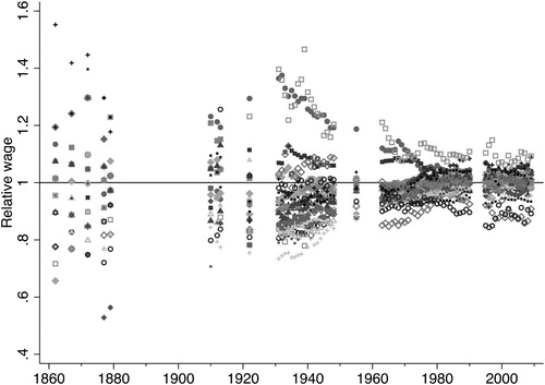
Figure 1 displays the nominal county wages relative to the nationwide mean.¹² A nominal county wage of 1.2 is equivalent to an advantage of 20% relative to the nationwide mean. The figure shows that the entire era featured a general tendency towards converging regional nominal wages. In the third quarter of the nineteenth century, county wages diverged from the nationwide mean by about 40%. The spread of wages diminished somewhat in the 1910s and 1920s. A massive decline took place between the 1930s and the 1970s, followed by a levelling out in the 1980s. Real county wages (not shown here) display a similar pattern. In sum, our wage evidence indicates a tendency towards regional wage convergence among the Swedish counties in 1860–2009, with some periods of exception. The pattern of wage dispersion for nominal and real wages was not, however, the same for all sub-periods.

Figure 1. Relative nominal county wages of male workers in manufacturing 1860–2009 (Sweden = 1). Source: See Appendix 1, Supplementary material; Regional employment: Enflo et al. (2014).

Note: The reference wage (Sweden) is the arithmetic mean of regional wages weighted by manufacturing employment up to 1990, thereafter by working hours.

Figure 2, which shows σ-convergence in nominal and real terms measured by the coefficient of variation, confirms our previous assessment of regional wage convergence.¹³ In nominal terms, a drastic decline in inter-county wage dispersion occurred during the 150-year period; the coefficient of variation fell from 15–20 to about 5% over the entire period.¹⁴ Wage convergence occurred most forcefully in the 1930s and 1940s; it also occurred from the mid-1870s to the early 1910s and from the mid-1960s to the early 1980s. Two periods stand out in contrast to the long-term trend of convergence: the years from the outbreak of World War I through the 1920s, which witnessed an increasing regional nominal wage dispersion; and the period after the early 1980s, during which the regional wage spread increased, especially in the years between 1983 and 1995.

Figure 2. The coefficient of variation for nominal and real county wages of male workers in manufacturing 1860–2009. Source: See Appendices 1–2, Supplementary material.

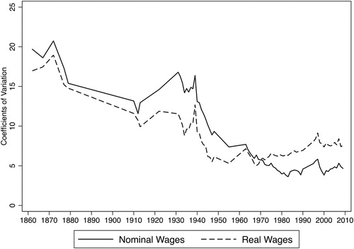
Figure 2 also displays the spread of real county wages, revealing the influence of regional cost of living on regional wage differences. The cost-of-living index employed was based on food prices, housing rents and other costs. In the first half of the period, variation in food prices accounted for most of the variation in cost of living; in the post-war period, especially from the 1970s onwards, housing rents gained importance relative to the total variation in cost of living. Our regional cost-of-living index shows the same tendency of σ-convergence displayed by wages, but the level of the coefficient of variation was lower and the convergence rate not so pronounced. Whereas regional differences in food prices tended to be very small throughout most of the era, differences in housing rents stemmed regional convergence in cost of living in the decades following World War II. For the period before World War I, when food prices weighed heavily as a share of total expenditures, our result is in line with the findings of previous studies (Bengtsson & Jörberg, 1981; Lundh, Schön, & Svensson, 2005).

As to real wages, Figure 2 indicates an overall decrease in county wage dispersion in the entire period, and in the sub-periods 1860–1912 and 1931–1945. It also indicates differences in the movements and levels of σ-convergence between real and nominal wages. First, when county nominal wages were deflated by county costs of living, the large increase in wage dispersion from the early 1910s to the early 1930s tended to disappear. For nominal wages, the decline in the regional wage spread continued through the 1970s, whereas the real wage dispersion seemed to have reached its lowest level by the end of the Second World War. We found no indication of regional real wage compression between 1945 and 1990. Second, from the late 1960s onwards, the level of dispersion was greater for real wages than for nominal wages. In the 1970s and early 1980s, nominal wage spread decreased, whereas real wage dispersion increased. Both followed a similar path thereafter, yet at different levels: regional differences were larger for real wages than for nominal wages. A number of factors might help explain these differences, such as the increasing importance of housing rents for cost of living and the continued regional variation in housing rents.

To further examine the overall trend and explore the patterns of sub-periods and groups of counties, we applied the two conventional tests for convergence of cross-sectional and time series data (Barro & Sala-i-Martin, 1991): σ-convergence and β-convergence.¹⁵ The test for σ-convergence is designed to capture the change in the spread of wages across counties over time, using the coefficient of variation (the standard deviation normalised by the mean) as a measure of wage dispersion. Whereas Figure 2 displayed all the coefficients of variation, Table 1 presents the results of the log-linear regression formula (1):(1) $\ln \left(C{V}_t\right)=\alpha +\text{β}\left(\mathrm{T}\mathrm{I}\mathrm{M}{\mathrm{E}}_t\right)+{\epsilon }_t$(1) where CV is the coefficient of variation at t, TIME is the order of time at t and ϵ is the error term at t. Sigma convergence occurs if the cross-sectional dispersion in wages declines over time. A negative and statistically significant coefficient for time indicates σ-convergence (Federico, 2012).

Table 1. Sigma-convergence regressions 1860–2009.

Period	Nominal wages		Real wages
	TIME		TIME
	(S.E.)	P > |t|	(S.E.)	P > |t|
1860/64–2009	−0,0133	0,000	−0,0059	0,000
	(0.0008)		(0.0007)
1860/64–1912	−0,0100	0,002	−0,0100	0,001
	(0.0015)		(0.0015)
1912–1931	0,0173	0,035	0,0072	0,236
	(0.0032)		(0.0043)
1931–1945	−0,0304	0,000	−0,0300	0,002
	(0.0045)		(0.0079)
1945–1968	−0,0191	0,000	−0,0001	0,820
	(0.002)		(0.0038)
1968–1983	−0,0339	0,000	0,0123	0,001
	(0.0018)		(0.0028)
1983–1995	0,0213	0,027	0,0174	0,000
	(0.0077)		(0.0027)
1995–2009	−0,0047	0,495	−0,0062	0,077
	(0.0067)		(0.0032)

Note: Following formula 1.

Sources: Appendices 1–2, Supplemental materials.

Table 1 shows that the coefficient for time for both nominal and real wages was negative and statistically significant relative to the long period 1860–2009, indicating the presence of σ-convergence overall. The table also shows that σ-convergence for both nominal and real wages took place in the sub-periods of 1860–1912, 1931–1945, 1968–1983 and 1995–2009. For the latter period, however, the coefficient for nominal wages was not statistically significant. As regards the period 1983–1995, our results indicate the same tendency towards divergence for nominal and real wages. Our regression results derived from real wage data did not confirm the results based on nominal wage data relative to two periods: we noticed divergence in 1912–1931 and convergence in 1945–1968.

In conclusion, we found an overall pattern of σ-convergence both for nominal and real wages during the period of investigation. Sometimes, however, our evaluation of specific sub-periods depends on the choice between nominal or real wages.

The test for β-convergence is designed to assess whether initially low-wage regions outgrow initially high-wage regions. It regresses the logged initial wage levels against the annual growth rates across a stipulated time span and singles out convergence through a negative coefficient. The test allows us to assess how fast a particular county's wage level is likely to catch up with the average wage level across all counties. In contrast, σ-convergence reveals how the distribution of wages across counties has behaved from an historical vantage point. In most cases, β-convergence and σ-convergence give similar insights into the rate of convergence or divergence. Manifest disturbances in the movement of wages may, however, lead to different conclusions regarding the rate of convergence because the estimated magnitude of β-convergence is particularly sensitive to the selected period. Our assessment will then be contingent on the convergence measure used (Barro & Sala-i-Martin, 1991; Carlino & Mills, 1996; Quah, 1993).

Figures 3 and 4 show the existence of β-convergence in nominal and real county wages between 1860 and 2009. The negative slopes of the figures testify to the catch-up potential among those lagging behind. In order to estimate the convergence rate, we employed formula (2) specified by Barro and Sala-i-Martin (1991) that often appears in studies of wage convergence (Collins, 1999; Roses & Sánchez-Alonso, 2004).¹⁶ It proceeds in two steps. First:(2) $\frac{1}{T}\ln \left(\frac{\mathrm{W}\mathrm{a}\mathrm{g}{\mathrm{e}}_{c,\mathrm{f}\mathrm{i}\mathrm{n}\mathrm{a}\mathrm{l}}}{\mathrm{W}\mathrm{a}\mathrm{g}{\mathrm{e}}_{c,\mathrm{i}\mathrm{n}\mathrm{i}\mathrm{t}\mathrm{i}\mathrm{a}\mathrm{l}}}\right)=\alpha +\theta \ln \left(\mathrm{W}\mathrm{a}\mathrm{g}{\mathrm{e}}_{c,\mathrm{i}\mathrm{n}\mathrm{i}\mathrm{t}\mathrm{i}\mathrm{a}\mathrm{l}}\right)+\gamma X_c+{\epsilon }_c$(2) where t is the first year in each sub-period, T is the number of years in each sub-period, and $\mathrm{W}\mathrm{a}\mathrm{g}{\mathrm{e}}_c$ is the average hourly wage of day workers in county c. The estimated regression coefficient, $\theta$, expresses the relation between growth rates and the level of the first year in natural logarithm. One may control for additional variables, $\gamma X_c$, as in the alternative specifications displayed in Tables 2 and 3, which add regional dummies and other variables capturing urbanisation, industrialisation and net-immigration in the counties. Formula (2) is thereby transformed from an unconditional to a conditional convergence model. The conditional model allows us to determine the extent to which the introduction of controls affects the estimated rate of convergence. If the controls reduce the size of $\theta$, one can conclude that they add to convergence. If, in contrast, the impact of controls increases the size of $\theta$, one can conclude that the controls add to divergence.

Figure 3. Annual growth rates of nominal county wages in 1860/4–2009 vs. the log of nominal county wages in 1860/4. Source: See Appendix 1, Supplementary material.

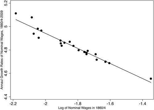
Figure 4. Annual growth rates of real county wages in 1860/1864–2009 vs. the log of real county wages in 1860/1864. Source: See Appendices 1–2, Supplementary material.

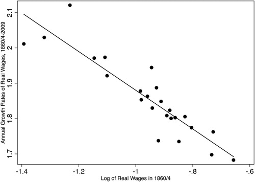
Table 2. Beta-convergence regressions 1860–2009, nominal wages.

Period	Model 1: Unconditional			Model 2: Conditional			Model 3: Conditional
	Conv. rate	P > |t|	R^2	Conv. rate	P > |t|	R^2	Conv. rate	P > |t|	R^2
	(S.E.)		(Prob > F)	(S.E.)		(Prob > F)	(S.E.)		(Prob > F)
1860/64–2009	0,0161	0,000	0,94	0,0173	0,000	0,94	0,0161	0,000	0,94
	(0.0003)		(0.000)	(0.0004)		(0.000)	(0.0004)		(0.000)
1860/64–1912	0,0337	0,000	0,55	0,0486	0,000	0,67	0,0647	0,000	0,66
	(0.0036)		(0.000)	(0.0037)		(0.001)	(0.0041)		(0.005)
1912–1931	0,0125	0,338	0,06	0,0203	0,239	0,16	0,0726	0,000	0,86
	(0.0112)		(0.338)	(0.0136)		(0.484)	(0.0059)		(0.000)
1931–1945	0,0345	0,000	0,77	0,0367	0,000	0,80	0,0354	0,000	0,80
	(0.0031)		(0.000)	(0.0036)		(0.000)	(0.0038)		(0.000)
1945–1968	0,0259	0,000	0,65	0,0247	0,000	0,66	0,0302	0,000	0,74
	(0.0030)		(0.000)	(0.0037)		(0.000)	(0.0036)		(0.000)
1968–1983	0,0568	0,000	0,66	0,0596	0,000	0,71	0,0327	0,052	0,68
	(0.0057)		(0.000)	(0.0062)		(0.000)	(0.0123)		(0.000)
1983–1995	−0,0170	0,163	0,09	−0,0191	0,171	0,09	−0,0207	0,125	0,30
	(0.0132)		(0.163)	(0.0153)		(0.566)	(0.0148)		(0.125)
1995–2009	0,0206	0,016	0,24	0,0212	0,025	0,24	0,0232	0,032	0,27
	(0.0068)		(0.016)	(0.0075)		(0.132)	(0.0084)		(0.181)

Note: Following formulas 2 and 3. Model 2 includes the geographical location (NUTS), and model 2 includes the variables: Industry's share of the total labour force; Percentage urban population, and Net of total migration (both external and internal).

Sources: Appendices 1–2, Supplemental materials.

Table 3. Beta-convergence regressions 1860–2009, real wages.

Period	Model 1: Unconditional			Model 2: Conditional			Model 3: Conditional
	Conv. rate	P > |t|	R^2	Conv. rate	P > |t|	R^2	Conv. rate	P > |t|	R^2
	(S.E.)		(Prob > F)	(S.E.)		(Prob > F)	(S.E.)		(Prob > F)
1860/64–2009	0,0107	0.000	0,81	0.0110	0.000	0.83	0.0109	0.000	0.85
	(0.0005)		(0.000)	(0.0005)		(0.000)	(0.0005)		(0.000)
1860/64–1912	0,0444	0.000	0,61	0.0474	0.000	0.63	0,0425	0.001	0.61
	(0.0035)		(0.000)	(0.0039)		(0.003)	(0.0040)		(0.010)
1912–1931	0,0696	0,001	0,52	0.0751	0.001	0.60	0.0758	0.000	0.92
	(0.0090)		(0.001)	(0.0091)		(0.004)	(0.0042)		(0.000)
1931–1945	0.0478	0.000	0,74	0.0478	0.000	0.74	0.0438	0.000	0.78
	(0.0044)		(0.000)	(0.0047)		(0.000)	(0.0047)		(0.000)
1945–1968	0.0301	0.002	0.36	0.0243	0.008	0.44	0.0239	0.009	0.50
	(0.0061)		(0.002)	(0.0063)		(0.008)	(0.0062)		(0.008)
1968–1983	0.0040	0.752	0.01	0.0069	0.581	0.16	0.0032	0.804	0.40
	(0.0120)		(0.752)	(0.0116)		(0.301)	(0.0124)		(0.039)
1983–1995	−0.0142	0.062	0.15	−0.0174	0.033	0.24	−0.0126	0.158	0.31
	(0.0080)		(0.062)	(0.0085)		(0.142)	(0.0094)		(0.121)
1995–2009	0.0117	0.049	0.17	0.0128	0.040	0.24	0.0115	0.136	0.21
	(0.0051)		(0.049)	(0.0053)		(0.128)	(0.0068)		(0.316)

Note and sources: See Table 2.

In the second step, the annual speed of convergence, β, is defined as in formula (3):(3) $\mathrm{A}\mathrm{n}\mathrm{n}\mathrm{u}\mathrm{a}\mathrm{l}\mathrm{s}\mathrm{p}\mathrm{e}\mathrm{e}\mathrm{d}\mathrm{o}\mathrm{f}\mathrm{c}\mathrm{o}\mathrm{n}\mathrm{v}\mathrm{e}\mathrm{r}\mathrm{g}\mathrm{e}\mathrm{n}\mathrm{c}\mathrm{e}\left(\text{β}\right)=-\left(\frac{1}{T}\right)\ln (\theta T+1)$(3) where $\theta$ is the regression coefficient from $\ln \left(\mathrm{W}\mathrm{a}\mathrm{g}{\mathrm{e}}_{c,\mathrm{i}\mathrm{n}\mathrm{i}\mathrm{t}\mathrm{i}\mathrm{a}\mathrm{l}}\right)$ in (2). Thus defined, the size of the coefficient is a positive value expressing the annual speed of convergence (Barro & Sala-i-Martin, 1991).

The region variable used as control is a dummy variable that assesses the importance of within-region β-convergence. In contrast, the unconditional model assesses the joint effects of within- and between-region convergence (Barro & Sala-i-Martin, 1991, 1995; Roses & Sánchez-Alonso, 2004). We classified counties as East, North or South according to level 1 of the classification scheme employed by NUTS. The North sample includes counties in Northern and Central Sweden, where the mining, wood and paper and pulp industries are common. The East and West sample include counties that have a more diversified industrial structure, barring the predominance of metal industries in the East. They also differ from the North with regard to the presence of large cities, such as Stockholm (East) and Gothenburg and Malmö (West).

The other controls include county statistics for industrialisation, urbanisation and migration. Industrialisation in the period 1860–1910 is represented by the proportion of the population who earned their living from industry; in the period 1920–1995, it is represented by the percentage of industrial workers among those who were employed.¹⁷ Urbanisation in the period 1860–1960 is represented by the city population's share of the total population; in the period 1960–1995, it is represented by the percentage of those among the total population who lived in densely populated areas (tätorter).¹⁸ Migration is represented by the total net immigration per 1000 in the mean county population, which is the difference between the internal and external in-migration minus the difference between the internal and external out-migration divided by the county population times 1000.¹⁹

Tables 2 and 3 display three models for the entire era and sub-periods based on formula (2). Model 1 estimates the speed of convergence without any controls (unconditional β-convergence). Model 2 adds controls for the region-specific growth rates of the North, East and West. Model 3 adds controls for county differences in the size of the industrial sector, the relative size of the urban population and the net total migration rate.

Table 2 displays the regression results for nominal wages. Starting with the unconditional Model 1 for the whole period, the estimate of β was 0.016 (p-value: 0.000). The average convergence rate for the full period was 1.6%. The high R² of 0.94 is implicit in the scatter plot of Figure 3, which shows the average growth of county wages in 1860–2009 against the natural log of the level of county wages in 1860. Model 2 estimated the speed of convergence after controlling for region-specific growth rates. The estimated β was 0.017 (p-value: 0.000). The similar sizes of the coefficients derived by Models 1 and 2 indicate that wages converged across regions and within each region at roughly the same speed. This result was largely the same after the inclusion of dummies for industrialisation, urbanisation and migration: Model 3 estimated β at 0.016 (p-value: 0.000).

Table 2 also shows the estimates of the convergence rates for sub-periods. The estimated β coefficient derived by Model 1 was positive and statistically significant. In line with the previous tests for σ-convergence (Table 1), it indicated β-convergence for all but two sub-periods, 1912–1931 and 1983–1995. The convergence rate ranged from 2 to 6%. Introducing geographical dummies (Model 2) did not produce significant changes. Even when we controlled for variations in the size of the industrial sector, urban population and in the net-total migration rate across counties (Model 3), the basic pattern remained the same, with one exception: Model 3 indicated a strong catch-up growth during the period 1912–1931, which differs from what Models 1 and 2 showed.

We now turn to the regression results for real wages, shown in Table 3. The long-term convergence rate was 1.1% for all three models. The sub periods displayed both differences and similarities compared to the pattern of nominal wages. We found similar indications of catch-up growth for the sub-periods 1860/1864–1912, 1931–1945, 1945–1968 and for the last sub-period 1995–2009. As for the period 1912–1931, however, the result for β- convergence was quite different for real wages compared to nominal wages. Interestingly, we found no indication of catch-up nominal wage growth, but we did find β-convergence for real wages. Much of this development was driven by increasing real wages in the counties of Stockholm, Gothenburg and Bohus, Malmöhus and Östergötland, which host important industrial cities such as Stockholm, Gothenburg, Malmö and Norrköping. This is probably the reason why we also found β-convergence for nominal wages when we controlled for the size of the industrial sector and the urban population (Model 3).

Results based on nominal and real wage data pointed in different directions relative to two sub-periods. For 1968–1983, we found β-convergence for nominal wages, but not for real wages. For 1983–1995, there was no catch-up wage growth, neither for nominal nor real wages. In regard to real wages, Table 3 shows clearly that the β-coefficient was negative and statistically significant for all models, indicating that high-wage counties outgrew low-wage counties during the period. As a consequence, county wage dispersion increased (see Table 1).

4. Discussion

Economic theory stipulates that workers with the same skill in a fully integrated labour market will receive equal wages regardless of geographic location. Yet the historical record shows us that payments have in fact varied across regions, hence suggesting that the condition of full integration has not been met. Labour markets of the past were in reality segmented and regional, rather than nationally integrated (Lundh et al., 2005; Rosenbloom, 1990; Roses & Sánchez-Alonso, 2004). The integration of labour markets began as new technologies of transports and communication facilitated mobility. We can see the empirical implication of market integration through evidence that shows a tendency of regional wage convergence.

The previous sections have shown that the trajectory of regional wage dispersion in Swedish manufacturing between 1860 and 2009 was marked by instances of strong σ-convergence and β-convergence, on the one hand, and instances of stability or divergence, on the other. The irregular convergence record since 1860 indicates that several different factors have affected wage dispersion interchangeably. In addition, convergence occurred in brief spells rather than by incremental shifts across long time spans. This episodic nature of convergence rules out any major influence of structural transformations. The years between 1860 and 2009 witnessed the rise and fall in the share of employment in manufacturing, as well as upswings and downswings in the shares of particular industries. Most of the estimated rates of β-convergence for different sub-periods remain after adding controls in terms of counties’ share of manufacturing employment and urbanisation. In Appendix 1, Supplementary material we provide additional evidence that compositional factors do not have a significant bearing on the estimated rate of σ-convergence. Whereas structural features appear to play a minor role, other county-specific experiences of convergence indicate the impact of several different factors. In the following discussion, we break down the entire era into four sub-periods and ascribe prominence to the historical factors that may have affected the spread of wages in each of them.

4.1. The first wave of convergence

Our results indicate a tendency towards regional wage convergence from the 1860s to the outbreak of World War I, both for nominal and real wages. Regional wage dispersion decreased and, on average, low-wage counties outgrew high-wage ones. Most international studies of pre-World War I regional wage dispersion have identified at least weak tendencies towards convergence (Table 4).²⁰ Some have even found wage convergence in the entire Atlantic economy, manifested through diminished wage gaps between the Old and the New World (Williamson, 1995).

Table 4. Periods of convergence and divergence for regional wages.

Study	Country	Occupational group	Convergence	Stable	Divergence
Hunt (1973)	Britain	Agrarian workers	1867/70–1898
		Bricklayers	1867/70–1898
Bengtsson and Jörberg (1981)	Sweden	Agrarian workers		1835/44–1890/99
Söderberg (1985)	Sweden	Agrarian workers		1840–1910
	France	34 professions and agrarian workers	1880–1910
	Britain	Agrarian workers	1840–1910
	Prussia	Unskilled workers		1840–1910
Rosenbloom (1990)	US	23 occupations	1870–1894
Boyer and Hatton (1994)	Britain	Agrarian workers			1855–1903
		Carpenters	1867–1913
Carlino and Mills (1995)	US	Per cap earnings	1931–1979		1979–1987
Heikkinen (1997)	Finland	Agrarian workers	1886–1913
Collins (1999)	India	Artisans		1873–1906
Roses and Sánchez-Alonso (2004)	Spain	Urban industrial workers	1854–1914		1914–1920
Barro and Sala-i-Martin (2004)	US	Personal incomes	1880–1920		1920–1930
			1930–1975		1975–1988
Barro and Sala-i-Martin (2004)	Japan	Personal incomes	1945–1980
Lundh et al. (2005)	Sweden	Industrial workers	1861–1913
Enflo et al. (2014)	Sweden	Agrarian workers	1860–1913		1913–1930
			1930–1940
Molinder (2017)	Sweden	Wage earners	1945–1957	1957–1967
			1967–1982
Collin, Lundh, and Prado (the current study)	Sweden	Manufacturing workers (nw)	1860–1912		1912–1931
			1931–1983		1983–2009
Collin, Lundh, and Prado (the current study)	Sweden	Manufacturing workers (rw)	1860–1912		1912–1931
			1931–1945	1945–1968	1968–2009

Researchers have emphasised two factors conducive to regional wage convergence in the 50 years preceding World War I, both falling under the rubric of factor mobility. First, the transport revolution united isolated areas and extended the geographical extent of each market. The construction of the Swedish railways in the 1870s established links between previously isolated and protected labour markets, providing jobseekers with opportunities on a permanent or casual basis in places other than their domicile or its immediate surroundings (Enflo, Alvarez-Palau, & Marti-Henneberg, 2018). The national government was responsible for the main railway lines connecting the large cities, whereas local authorities and private stakeholders invested in meshing smaller population centres. A tightly knit network of local railway lines would eventually crisscross Sweden in the interwar years. Moreover, the postal service, the telegraph and the telephone revolutionised personal communications (Andersson-Skog, 2002; Kaijser, 1994).

Second, labour mobility increased, both internally and externally. Short-distance and circular migration was dominant in Sweden and in other countries, so that long-distance moves were quite rare. But the opening of new regional labour markets in industrial and urban areas along with improvements in transportation stimulated long-distance migration. In 1860, on average 7% of the population were born outside their county of residence (Institute for Social Sciences, 1941, p. 42; Lundh, 2006). In 1900 and 1930, the corresponding percentage points were 16 and 22, respectively, indicating a substantial increase in long-distance internal migration. Large differences prevailed among counties, however, and the city of Stockholm hosted a population of 60% in-migrants throughout the period. When it comes to external labour mobility, the sheer size of the emigration of Swedish workers to the US is worthy of attention, which has often led economic historians to assume that emigration had a powerful effect on the rewards of labour (Bohlin & Eurenius, 2010; Hatton & Williamson, 1998, pp. 197–198). Unsurprisingly, emigration diminished the supply of labour relative to other factors of production in the late nineteenth and early twentieth centuries (O’Rourke & Williamson, 1999). Enflo, Lundh, and Prado (2014) provide econometric evidence that emigration and internal migration before World War I diminished regional wage differentials. Emigrants left above all low-wage counties. The diminished supply of workers in low-wage counties spurred faster growth rates of wages in them than in high-wage counties, which resulted in declining wage differentials across all counties.

A different strand of literature on the role of labour mobility and convergence has argued that a large inflow of workers to the cities may push spatial divergence forward. In the jargon of new economic geography, so-called agglomeration effects in densely populated areas may have growth-enhancing effects, mitigating the downward pressure on wages in the receiving areas. Some of these agglomeration effects are, for instance, attributes such as immigrants’ age, skills, and entrepreneurship (Kanbur & Rapoport, 2005). It is not likely, however, that such agglomeration effects were particularly strong in Sweden in the late nineteenth and early twentieth century. The early Swedish industrialisation was mainly a rural phenomenon until the beginning of the twentieth century (Berger, Enflo, & Henning, 2012); labour mobility spurred convergence, overwhelming the dispersive role of agglomeration forces over wages.

4.2. Interruption

Wage convergence was interrupted during the First World War and throughout the 1920s. We found a tendency towards diverging nominal wages across counties in Swedish manufacturing from the early 1910s to the 1930s. Regional real wage dispersion was quite stable, however, and the process of catch-up growth continued. The tendency of divergence also applied to farm workers’ wages and to the urban to rural wage ratio, as recent research has shown (Lundh & Prado, 2015; Prado, Collin, Lundh, & Enflo, 2016). Few studies on regional wage convergence across the interwar years have been published. Roses and Sánchez-Alonso (2004) found divergence in Spain between 1914 and 1920, whereas Barro and Sala-i-Martin (1991) noticed divergence only in the 1920s. Carlino and Mills (1996) American study started only in 1931, showing converging wages henceforth.

World War I and the economic crisis of the early 1920s halted convergence for some time. Emigration almost ceased during the war and remained low in the 1920s. Enflo et al. (2014) have shown that emigration during the interwar years did not contribute to wage convergence as it had before the war. As a result of the severe deflation in the early 1920s, wages in industries either susceptible to, or shielded against, world market competition followed different paths. Nominal wages for workers in the traded goods sector fell deeper than wages for workers in the non-traded goods sector (Bengtsson & Molinder, 2017; Fregert, 1994). The wage advantage of workers in the non-traded goods sector increased from 5 to 30% between 1920 and 1921 (Fregert, 1994, p. 174). As traded and non-traded goods industries were not evenly distributed across counties, this development influenced regional wage dispersion.

4.3. The second wave of convergence

The second wave of converging regional wages in manufacturing occurred in the 1930s and 1940s, and it was notably strong. For nominal wages in particular, convergence at lower rates continued through the 1960s and 1970s. Prado et al. (2016) painted a similar picture of convergence of agrarian workers in Sweden between 1930 and 1980. Most previous international studies have also found regional wage convergence in this time span. Carlino and Mills (1996) have noticed converging regional wages for the US from 1931 to 1979 and Barro and Sala-i-Martin (1991) found converging regional GDP per capita in the US for almost the same time span (1930–1975). The only study whose findings clash with our chronological account of convergence is Roses and Sánchez-Alonso’s (2004). Examining Spanish regional wages, they argue that convergence occurred as early as in the 1920s. It is important to note, however, that previous studies have not controlled for regional differences in cost of living. When such differences are taken into account, the indication of σ-convergence tends to disappear, as we have shown for the Swedish case, despite the evidence of β-convergence up to the 1970s.

Labour migration, instrumental in the first wave of regional wage convergence (Enflo et al., 2014), was probably inconsequential in the second wave. Emigration to the US declined in the 1920s, ceasing in the 1930s. Internal migration decreased as a result of the economic crisis of the early 1920s and remained low until the second half of the 1930s, which suggests that it was not an evident driver of regional wage convergence in the 1930s either. Molinder (2017, 2018) examines the period 1945–1985 and concludes that the role played by regional earnings differences in net internal migration was secondary; instead, he lays emphasis on the pace and direction of structural change.

Immigration might have influenced wage convergence. During World War II, Sweden received refugees from the Nordic and Baltic countries. The war was followed by quite a long period of immigration of foreign workers into the Swedish industry, which ended in the late 1960s, when immigration policy was subjected to restrictions (Lundh & Ohlsson, 1997). At the general level, immigration put a downward pressure on wages by increasing the labour supply. Between 1946 and 1967, 60% of the immigrants went to the counties of Stockholm, Gothenburg, Malmö and Västmanland, all of which were important industrial areas offering wage levels at the upper end of the scale. Other high-wage counties, such as Norrbotten and Västerbotten in the north, received only 1–2% of the immigrants. On average, the correlation between the county nominal wage level and the percentage of immigrants received was about 60%.²¹ It is thus probable that immigration contributed to the regional convergence in nominal wages by supplying extra labour to areas with great demand for labour in the post-war period.

Yet the main potential driver of the Swedish regional wage convergence in the 1930s and 1940s was collective bargaining. Its crucial mechanism was the implementation of nationwide collective agreements that were specific to each industry and evened out within-industry differences in wages across regions. Unlike Britain, in which unions were organised by occupation, trade unions and employers in Sweden were largely organised by industry (Lundh, 2010). Before World War I, union density was still quite low (about 15%), but since the collective agreements also included non-union members employed by firms that practiced collective bargaining, they covered in fact about half of the working force in manufacturing. Unionism increased rapidly during the interwar period; around 1930, half of the blue-collar workers in the manufacturing industry were union members. The coverage of the collective agreements reached up to 60–80%, depending on the industrial branch (Lundh, 2010, p. 105).

The centralised agreements became more important during the first half of the twentieth century. In the beginning of the century, wage formation was local and laid down in collective agreements between trade unions and firms/local employers’ associations. Few nationwide collective agreements standardised employment conditions and working hours. During the interwar period, the Swedish Employers’ Confederation (Svenska Arbetsgivareföreningen, SAF), a strong advocate of nationwide wage formation, rallied to include wages in the national collective bargaining. As a result, nationwide agreements across industries became more common. SAF advocated nationwide agreements because standardised employment conditions, in terms of working hours and wages, would prevent local firms from competing for labour. SAF's policy also stemmed other types of ‘unfair’ competition within and across industrial branches.

Collective bargaining was not restricted to norms governing within-industry wage harmonisation; trade unionist norms that favoured increasing wage equality between occupational groups and across industries were also part of the collective bargaining system. A wage equality policy was introduced during World War II and practiced from the 1950s through the 1970s. The centralised agreements between The Swedish Confederation of Trade Unions (Landsorganisationen i Sverige, LO) and SAF, which aimed to curb inflation during the initial phases of World War II, generated a levelling of between-industry wage differentials. The agreements stipulated that only low-wage industries would be fully compensated for a rising cost of living. A corollary to this particular aspect of the wage policy was that low-wage industries outgrew high-wage ones. Recent research argues that wage alignment during the war was a predecessor of the so-called solidaristic wage policy that would be put into practice in the 1950s (Collin, 2016; Prado & Waara, 2018). The compression of inter-industry wage differentials caused by the centralised agreements is key to understanding the rapid second-wave decline in regional wage differentials revealed in this study.

If the centralised agreement aiming at wage compression during World War II was episodic, the similar policy that emerged in the 1950s was long lasting. LO accepted a new policy governing wage dispersion in 1951, after years of pressure from low-wage groups and unions. The so-called solidaristic wage policy aimed to compress the industrial wage structure in collective bargaining by allowing the low-wage groups to have a larger rise in payments. Coordinated collective bargaining for the entire industrial labour market was a prerequisite. The two most important parties in the industrial labour market were keen to keep wage dispersion within a certain range. Coordinated collective bargaining, leading to a nationwide collective agreement at the industry level, was implemented in 1952 and practiced uninterruptedly from 1956 to 1982 (Lundh, 2010; Ullenhag, 1971). The impact of the solidaristic wage policy on wage levelling was strongest in the 1970s (Hibbs, 1991; Molinder, 2017, 2018).

In conclusion, the institutional setup of the labour market played a central role in the second wave of regional wage convergence in manufacturing. Nationwide wage formation at the industry level was closely associated with the pronounced decrease in regional wage dispersion in the 1930s and 1940s. In addition, the system of coordinated collective bargaining along with the solidaristic wage policy of the late 1960s and 1970s further diminished the wage spread, which probably led to the decrease of nominal wage differentials.

4.4. Levelling out

Nominal wage convergence in the late twentieth and early twentieth-first centuries showed a slightly different pattern in comparison with the previous sub-periods. After reaching an average CV of about 5% in the early 1980s, regional nominal wage dispersion did not decline as dramatically. As for regional real wages, the CV appeared to have stabilised at an equally low level already by the 1960s, perhaps as early as by the 1940s. Despite these differences between the nominal and real terms, it is reasonable to conclude that from the early 1980s to the end of the studied period the level of regional wage variation was low with a slightly increasing tendency, in particular between mid-1980s and mid-1990s. The tendency of regional wages towards divergence finds support in studies that look at regional GDP in the US and Sweden in the post-1980 period (Barro & Sala-i-Martin, 2004; Carlino & Mills, 1996; Enflo & Rosés, 2015).

Regional variation was larger in real wages than in nominal wages, which stemmed from the increasing importance of housing rent in the cost-of-living index. This result indicates that housing expenditures had to some extent become disconnected from conditions in the labour market. Still, the spread of regional wages, real and nominal, remained very low. Studies of regional GDP, in contrast, record more significant divergence in the post-1980 period (Enflo & Rosés, 2015). This is an expected outcome against the backdrop of several macro-economic disturbances, such as the oil crises of the 1970s and the economic crisis of the early 1990s. In addition, globalisation and the ICT revolution are likely to have influenced labour supply and demand differently across industries and locations.

The different patterns of nominal and real wage dispersion may be puzzling. It should be noted, however, that regional wage dispersion was a side effect of wage formation both on the local, industry level and on the national level. The centralised collective bargaining system shaped the development of wages both at the local, industry level and the national level, establishing wage levels for firms and workers regardless of geographical location. Besides, the solidaristic wage policy regulated earnings differences between workers within one industry or across industries nationwide, and it did not take into full account cost-of-living differentials across regions. The focus was on the national average rather than the regional variation.

We cannot exclude the potential role of ignorance about the development of regional cost of living from the 1960s onwards. Geographic differences in cost of living were an important issue during World War I, and in the early 1920s the Social Board categorised local communities according to the level of cost of living into a seven-stage hierarchy. As regional price variation tended to decrease, fewer and fewer categories of local cost-of-living levels were used. There was consensus in the 1960s that regional price differences were very small, and in the 1970s the attempt to measure regional cost of living was abandoned. By that time, regional variation in housing costs started to rise.

A pertinent question is which factors constrained the spread of wages. A possible answer should consider the nationwide character of the Swedish collective bargaining. It is likely that the same wage alignments responsible for most of the compression since the early 1930s have also provided a bulwark against mounting regional inequality forces since the early 1980s.

Labour mobility and centralised wage formation have almost wiped out all of the Swedish regional wage differentials in manufacturing; the wage spread has become so low that additional convergence is unlikely. The differences that persist may reflect pecuniary advantages in compensation for inferior site-specific characteristics. For instance, a significant wage premium might attract manufacturing workers to Norrbotten, the northernmost county of Sweden, despite the darkness and the cold weather. In a similar way, manufacturing workers in Stockholm may accept a real wage penalty caused by higher housing costs in return for the ample job opportunities and leisure pursuits that the capital offers.

5. Conclusion

Economic theory predicts small wage differentials among workers and geographic locations, provided that human capital does not vary much. In practice, however, labour markets of the past have failed to confirm this prediction: there is consistent evidence that large wage differentials across space were commonplace. Swedish manufacturing in the third quarter of the nineteenth century was no exception. The very long period considered here, from 1860 to 2009, has allowed us to document the long-term tendency of σ-convergence displayed by the evolution of regional wage dispersion in Swedish manufacturing. The spread of wages was a great deal larger in the 1860s than in the 2000s. In addition, we have shown that regional wage compression also manifested itself through β-convergence, that is to say, low-wage regions caught up with high-wage regions. This result remained the same after controlling for the impacts of within-region convergence, migration, urbanisation and industrialisation.

Two distinct instances of convergence, interrupted by brief spells of divergence or stability, steered the regional wage dispersion throughout the entire era. The first of those spells occurred before the outbreak of World War I and was associated with increased labour mobility, made possible by improved transportation and communication technologies and by the establishment of a modern labour market. The emblematic example of labour mobility was emigration, which accelerated wage growth rates among low-wage counties. The second spell of convergence occurred in the 1930s and during World War II, and continued at a lower rate for nominal wages through the 1970s. This wave of convergence was associated with the collective wage formation system characteristic of the Swedish model, characterised by high levels of union membership and collective agreement coverage, centralised wage formation and policies aiming at a decrease in wage differences.

Even though the patterns of regional wage dispersion might look similar for nominal and real wages in many cases, we show that the two dispersion measures may diverge. When we controlled for regional cost differentials, the real dispersion measure did not decline in the post-1970 period. By then, housing costs began to weigh more heavily in the household budget and regional differences in housing costs were less associated with levels of regional nominal earnings than previously. To our knowledge, this is the only study that compares the nominal and real wage dispersion over a long period. Our results invite further efforts to examine the long-run behaviour of nominal and real dispersion across regions.

Acknowledgements

Earlier versions of this paper were presented at: the FRESH meeting in Dublin, 2014; the Swedish Economic History Meeting in Stockholm, 2017; and the Higher Seminar in Economic History, University of Gothenburg. We appreciate all the suggestions from the participants. We are also thankful for the invaluable comments by Sakari Heikkinen, Rodney Edvinsson, Stefan Öberg and Jan Bohlin, who read a previous version of this paper and for the comments and suggestions of three anonymous reviewers. We also thank Evelyn Prado for proof reading. We would like to acknowledge the financial support from Riksbankens Jubileumsfond and Jan Wallanders och Tom Hedelius Stiftelse/Tore Browaldhs Stiftelse, for the research projects ‘Swedish Wages in Comparative Perspective, 1860–2008’ (P09-0500:11-E) and ‘Swedish Wages 1860–2010 in labour economics perspective’ (P2011-0182:1). Kristoffer Collin and Svante Prado would also like to acknowledge individual financial support provided by Jan Wallanders och Tom Hedelius Stiftelse (W17-0032; W2009-0161:1).

Disclosure statement

No potential conflict of interest was reported by the authors.

Additional information

Funding

This work was supported by Jan Wallanders och Tom Hedelius Stiftelse samt Tore Browaldhs Stiftelse [grant number P2011-0182:1, W17-0032, W2009-0161:1]; Riksbankens Jubileumsfond [grant number P09-0500:1-E].

Notes

1 Wage convergence in itself is, however, neither a necessary nor a sufficient premise to establish the occurrence of labour market integration (Boyer & Hatton, 1997, p. 724; Rosenbloom, 1998, p. 291).

2 Workers may be willing to accept different levels of compensation depending on the value they place on site-specific attributes (Eberts & Schweitzer, 1994), on the relatively higher risk of unemployment in urban areas (Hatton & Williamson, 1992; Todaro, 1969) or on other disamenities associated with city life, such as shorter life expectancy, higher infant mortality, and poorer environmental quality (Williamson, 1981).

3 On wage convergence across regions, see, for instance: Rosenbloom (1990, 1998, 2002); Collins (1999); Roses and Sánchez-Alonso (2004); Margo (1999); Boyer and Hatton (1997); Bengtsson and Jörberg (1981); Bengtsson (1990); Söderberg (1985); Lundh et al. (2005); Sicsic (1995); Heikkinen (1997, p. 135); Verma (1973). On convergence across countries and continents, see, for instance: Curtis and Fitz Gerald (1996); Williamson (1995); Allen (1994); Prado (2010a); Caruana Galizia (2015, p. 122).

4 From the very beginning in 1913, the official wage statistics of industrial workers excluded all salaried employees from the reported means by industry. Monthly earnings of salaried employees were reported under the heading ‘clerical staff’ (Förvaltningspersonal), and the reported means were not distinguished by industry.

5 Appendix 1, Supplementary material displays two tests of the effects of compositional changes: (i) the shares of manufacturing employment across counties; and (ii) the shares of employment across industries within counties. The tests, reported in Table A.1.1 and Table A.1.2, show that these compositional effects are small. They do not have a significant impact on the estimated rate of sigma convergence.

6 In the case of Stockholm, the official statistics distinguish between Stockholm city (urban) and Stockholm county (rural) until 1967. In order to make the data homogeneous, we merged those geographical units, which resulted in 24 counties.

7 The Historical Labour Database (HILD) includes detailed bibliographic references to the official statistics. Retrieved from http://es.handels.gu.se/avdelningar/avdelningen-for-ekonomisk-historia/historiska-lonedatabasen-hild.

8 We adopted the following procedure in order to examine whether the benchmarks of 1910, 1912 and 1913 were indicative of manufacturing at large: First, we established a CV for the mechanical engineering industry in 1922. The CV was 18.8%, that is, larger than the economy-wide CV of 14.3%. Second, we repeated this exercise for 1879; again, the CV of 20.7% for the mechanical engineering industry was larger than the economy-wide CV of 16.3%. Hence, we may overestimate the spread of wages by about 4 percentage points in the benchmarks of 1910, 1912 and 1913.

9 The filled-out forms included geographical information that the Social Board did not use in the published tables.

10 In 1997, Skåne county was established by merging Kristianstad county and Malmöhus county; in 1998, Västra Götaland county was established by merging Göteborg och Bohus county, Älvsborg county and Skaraborg county.

11 Industry-specific county wages are scarce for the benchmark of 1990; wages were not reported for the leather, hair and rubber industry because rubber manufacturing was incorporated into the chemical industry in 1971, and leather manufacturing was incorporated into the textile and clothing industry in 1975. Our sample of industry-specific county wages in 1990 comprised 100 wage observations, thus covering roughly 60% of the potential total sample (168 wage observations).

12 In the early 1860s, the mean hourly payment of male workers in manufacturing was 0.16 Swedish krona (SEK). It increased to 173.37 SEK in 2009, implying a growth rate of 4.83% per year for the entire period. The corresponding growth rate for real wages was 1.86. Prado’s (2010b) estimated growth rate for wages in manufacturing at large is very similar.

13 Besides the coefficient of variation, studies of σ-convergence also use the standard deviation of the log of wages or log of income per worker. Sometimes the two measures give different results (Dalgaard & Vastrup, 2001). We have used our nominal wage series to cross-check the differences yielded by the two measures. For the period as a whole, it makes almost no difference which measure we use. If we set the two measures to 100 in 1860, the difference in 2009 is one percentage point: the coefficient of variation arrives at 23.7 and the standard deviation of the log of wages arrives at 24.6. The only noteworthy difference between the two measures relates to the 1870s, when the log of standard deviation indicates stronger convergence than the coefficient of variation.

14 For the sake of simplification, we have avoided reproducing the four time spans specified by the Tariff Commission, namely, 1860–1864, 1865–1869, 1870–1874 and 1875–1879. Instead, we refer to the year in the middle of each time span: 1862, 1867, 1872 and 1877.

15 Unlike Islam (1995), we do not compute convergence by panel data regressions because of irregularities in our cross sections over time. Besides, as we have yearly data only for part of the period of investigation, we did not apply any test for stochastic convergence (e.g. co-movement or co-integration) using time series data (Carlino & Mills, 1996; Federico, 2012). In other words, we test only Cournot's law of one price, and not market efficiency.

16 According to Barro and Sala-i-Martin (1995, p. 387), the average growth rate over a period of T years for region i can be written as follows: $\left(1/T\right)\ln \left(Y_{iT}/Y_{i0}\right)=a-\left[(1-e^{-\text{β}T})/T\right]\ln Y_{i0}+u_i$, where Y is income per capita, a is a constant, $\text{β}$ is the convergence rate, and u is an error term.

17 County population: Statistics Sweden: Historisk statistik, 1, Table 5 (1860–1967) and Statistical Database (1968–1995). Industry population: Statistics Sweden: Folkräkningen (BiSOS A, 1860; SOS, 1910–1970), Folk- och bostadsräkningen (SOS, 1965–1970), and Statistical Database (1968–1995).

18 Statistics Sweden: Historisk statistik, 1, Table 7; Tätorter 1960–2005. Statistiska Meddelanden MI 38 SM 0703.

19 1860–1968: Hofsten and Lundström (1976, Table 8.2, p. 142); 1983 and 1995: Statistics Sweden, Statistical Database.

20 For Sweden, see, for instance: Lundh et al. (2005); Bengtsson and Jörberg (1981); Bengtsson (1990); Enflo et al. (2014); Prado et al. (2016). For other countries, see, for instance: Roses and Sánchez-Alonso (2004); Heikkinen (1997); Boyer and Hatton (1997); Caruana Galizia (2015); Rosenbloom (1998).

21 Our calculation, based on SOS Befolkningsrörelsen, Folkmängdens förändringar, Befolkningsförändringar.

References

- Archives
- National Archives (Riksarkivet), Stockholm
- Tullkommittén [Tariff Commission]. (1876). Sammandrag av svar och frågeformulär; Vols. 3–6. Ref. code: SE/RA/310791.
- Socialstyrelsens 5:e byrån [Social Board’s 5th Bureau]. H4ABA Löneförhållanden inom industrin, byggnadsindustrin, förvaltning m.m 1913–1961; Vols. 7–11 (1922) and 386–391 (1955); Ref. code: SE/RA/420267/420267.06.
- Centre for Business History (Centrum för näringslivshistoria), Stockholm
- Sveriges Verkstadsförening [the Swedish Metal Trades Employers’ Association], Föreningen Teknikföretagen. Allmän lönestatistik 1910, Vol. F13ba:4; Allmän lönestatistik 1912, Vol. F13ba:6; Allmän lönestatistik 1913, Vol. F13ba:7.
- Official publications
- Befolkningsförändringar. Sveriges Officiella Statistik (SOS). Stockholm: Statistiska Centralbyrån (SCB).
- Befolkningsrörelsen. SOS. Stockholm: SCB.
- Detaljpriser och indexberäkningar åren 1913–1930. Stockholm: Socialstyrelsen [Social Board], 1933.
- Folk- och bostadsräkningen 1965, 1975. SOS. SCB: Stockholm.
- Folkmängdens förändringar. SOS. Stockholm: SCB.
- Folkräkningen 1860. Bidrag till Sveriges Officiella Statistik [Contributions to the Swedish Official Statistics] (BiSOS) A. Stockholm: SCB.
- Folkräkningen 1910–1970. SOS. Stockholm: SCB.
- Historisk statistik för Sverige. Del 1. Befolkning. Andra upplagan 1720–1967. Stockholm: SCB, 1969.
- Hofsten, E. and H. Lundström (1976). Swedish Population History. Main trends from 1750 to 1970. Urval, no. 8. Stockholm: SCB.
- Konsumentpriser och indexberäkningar 1931–1959. Stockholm: Socialstyrelsen, 1961.
- Statistiska Meddelanden MI 38 SM 0703.
- Digital sources
- Historical Labour Database (HILD) [Historiska lönedatabasen]. Retrieved from http://es.handels.gu.se/avdelningar/avdelningen-for-ekonomisk-historia/historiska-lonedatabasen-hild
- Statistics Sweden: Statistical Database [Statistikdatabasen. SCB]. Retrieved from www.statistikdatabasen.scb.se
- Books and articles
- Allen, R. C. (1994). Real incomes in the English speaking world, 1879–1913. In G. Grantham & M. McKinnon (Eds.), Studies in the evolution of labour markets in the industrial era (pp. 107–138). London: Routledge.
- Andersson-Skog, L. (2002). Från normalspår till bredband: svensk kommunikationspolitik i framtidens tjänst 1850–2000. In L. Andersson-Skog & O. Krantz (Eds.), Omvandlingens sekel: perspektiv på ekonomi och samhälle i 1900-talets Sverige (pp. 117–143). Lund: Studentlitteratur.
- Barro, R., & Sala-i-Martin, X. (1995). Economic growth. New York: McGrawHill.
- Barro, R., & Sala-i-Martin, X. (2004). Economic growth (2nd ed.). Cambridge, MA: MIT Press.
- Barro, R. J., & Sala-i-Martin, X. (1991). Convergence across states and regions. Brookings Papers on Economic Activity, 1991(1), 107–182.
- Bengtsson, T., & Jörberg, L. (1981). Regional wages in Sweden during the nineteenth century. In P. Bairoch & M. Lévy-Leboyer (Eds.), Disparities in economic development since the industrial revolution (pp. 227–243). London: The Macmillan Press.
- Bengtsson, E., & Molinder, J. (2017). The economic effects of the 1920 eight-hour working day reform in Sweden. Scandinavian Economic History Review, 65(2), 149–168.
- Bengtsson, T. (1990). Migration, wages, and urbanization in Sweden in the nineteenth century. In A. van der Woude, A. Hayami, & J. de Vries (Eds.), Urbanization in history: A process of dynamic interactions (pp. 186–204). Oxford: Clarendon Press.
- Berger, T., Enflo, K., & Henning, M. (2012). Geographical location and urbanisation of the Swedish manufacturing industry, 1900–1960: Evidence from a new database. Scandinavian Economic History Review, 60(3), 290–308.
- Bohlin, J., & Eurenius, A.-M. (2010). Why they moved — Emigration from the Swedish countryside to the United States, 1881–1910. Explorations in Economic History, 47(4), 533–551.
- Boyer, G. R. & Hatton, T. J. (1994). Regional labour market integration in England and Wales, 1850–1913. Cornell University.
- Boyer, G. R., & Hatton, T. J. (1997). Migration and labour market integration in late nineteenth-century England and Wales. The Economic History Review, 50(4), 697–734.
- Carlino, G., & Mills, L. (1996). Convergence and the U.S States: A time-series analysis. Journal of Regional Science, 36(4), 597–616.
- Caruana Galizia, P. (2015). Mediterranean labor markets in the first age of globalization: An economic history of real wages and market integration. New York: Palgrave Macmillan.
- Coelho, P. R. P., & Shepherd, J. F. (1974). Differences in regional prices: The United States, 1851–1880. The Journal of Economic History, 34(3), 551–591.
- Collin, K. (2016). Regional wage gaps between agricultural and manufacturing workers in Sweden, 1860–1945. In K. Collin (Eds.), Regional wages and labour market integration in Sweden, 1732–2009 (pp. 117–158). Gothenburg Studies in Economic History, No. 17. Gothenburg: Gothenburg University.
- Collins, W. J. (1999). Labor mobility, market integration, and wage convergence in late 19th century India. Explorations in Economic History, 36(3), 246–277.
- Cournot, A. (1971). Mathematical principles of the theory of wealth. New York: Macmillan.
- Curtis, J., & Fitz Gerald, J. D. (1996). Real wage convergence in an open labour market. Economic and Social Review, 27(4), 321–340.
- Dalgaard, C.-J., & Vastrup, J. (2001). On the measurement of σ-convergence. Economics Letters, 70(2), 283–287.
- Eberts, R. W., & Schweitzer, M. E. (1994). Regional wage convergence and divergence: Adjusting wages for cost-of-living differences. Economic Review, 30(2), 26–37.
- Enflo, K., Alvarez-Palau, E., & Marti-Henneberg, J. (2018). Transportation and regional inequality: The impact of railways in the Nordic countries, 1860–1960. Journal of Historical Geography, 62, 51–70.
- Enflo, K., Lundh, C., & Prado, S. (2014). The role of migration in regional wage convergence: Evidence from Sweden 1860–1940. Explorations in Economic History, 52(2), 93–110.
- Enflo, K., & Rosés, J. R. (2015). Coping with regional inequality in Sweden: Structural change, migrations, and policy, 1860-2000. The Economic History Review, 68(1), 191–217.
- Federico, G. (2012). How much do we know about market integration in Europe. The Economic History Review, 65(2), 470–497.
- Fregert, K. (1994). Relative wage struggles during the interwar period, general equilibrium and the rise of the Swedish model. Scandinavian Economic History Review, 42(2), 173–186.
- Gärtner, S. (2016). New Macroeconomic evidence on internal migration in Sweden, 1967–2003. Regional Studies, 50(1), 137–153.
- Hatton, T. J., & Williamson, J. G. (1991). Unemployment, employment contracts, and compensating wage differentials: Michigan in the 1890s. The Journal of Economic History, 51(3), 605–632.
- Hatton, T. J., & Williamson, J. G. (1992). What explains wage gaps between farm and city? Exploring the Todaro model with American evidence, 1890–1941. Economic Development and Cultural Change, 40(2), 267–294.
- Hatton, T. J., & Williamson, J. G. (1993). Labour market integration and the rural-urban wage gap in history. In G. D. Snooks (Ed.), Historical analysis in economics (pp. 89–109). London: Routledge.
- Hatton, T. J., & Williamson, J. G. (1998). The age of mass migration: Causes and economic impact. Oxford: Oxford University Press.
- Heikkinen, S. (1997). Labour and the market: Workers, wages and living standards in Finland, 1850–1913. Helsinki: The Finnish Society of Sciences and Letters.
- Hicks, J. R. (1932). The theory of wages. London: Macmillan.
- Hibbs, D. A. Jr. (1991). Market forces, trade union ideology and trends in Swedish wage dispersion. Acta Sociologica 34:89–102.
- Hunt, E. H. (1973). Regional wage variations in Britain, 1850–1914. Oxford: Clarendon Press.
- Institute for Social Sciences, U. o. S. (1941). Population movements and industrialization: Swedish counties, 1895–1930. London: P.S. King.
- Islam, N. (1995). Growth empirics: A panel data approach. The Quarterly Journal of Economics, 110(4), 1127–1170.
- Kaijser, A. (1994). I fädrens spår: den svenska infrastrukturens historiska utveckling och framtida utmaningar. Stockholm: Carlssons.
- Kanbur, R., & Rapoport, H. (2005). Migration selectivity and the evolution of spatial inequality. Journal of Economic Geography, 5(1), 43–57.
- Lundh, C. (2006). Arbetskraftens rörlighet och arbetsmarknadens institutioner i Sverige 1850–2005. In D. Rauhut & B. Falkenhall (Eds.), Arbetsrätt, rörlighet och tillväxt (pp. 17–62). Östersund: ITPS.
- Lundh, C. (2010). Spelets regler: institutioner och lönebildning på den svenska arbetsmarknaden 1850–2000 (2nd ed.). Stockholm: SNS.
- Lundh, C., & Ohlsson, R. (1997). Från arbetskraftsimport till flyktinginvandring (2nd ed.). Stockholm: SNS.
- Lundh, C., & Prado, S. (2015). Markets and politics: The Swedish urban-rural wage gap, 1865–1985. European Review of Economic History, 19(1), 67–87.
- Lundh, C., Schön, L., & Svensson, L. (2005). Regional wages in industry and labour market integration in Sweden, 1861–1913. Scandinavian Economic History Review, 53(3), 71–84.
- Margo, R. A. (1999). Regional wage gaps and the settlement of the Midwest. Explorations in Economic History, 36(2), 128–143.
- Marshall, A. (1920). Principles of economics. London: Macmillan.
- Molinder, J. (2017). Interregional migration, wages and labor market policy: Essays on the Swedish model in the postwar period. Uppsala: Uppsala University.
- Molinder, J. (2018). Why did Swedish regional net migration rates fall in the 1970s? The role of policy changes versus structural change, 1945–1985. Scandinavian Economic History Review, 66(1), 91–115.
- O’Rourke, K. H., & Williamson, J. G. (1999). Globalization and history: The evolution of a nineteenth-century Atlantic economy. Cambridge, MA: MIT Press.
- Prado, S. (2010a). Fallacious convergence? Williamson’s real wage comparisons under scrutiny. Cliometrica, 4(2), 171–205.
- Prado, S. (2010b). Nominal and real wages of manufacturing workers, 1860–2007. In R. Edvinsson, T. Jacobsson, & D. Waldenström (Eds.), Exchange rates, prices, and wages, 1277–2008 (pp. 479–527). Stockholm: Ekerlids förlag.
- Prado, S., Collin, K., Lundh, C. & Enflo, K. (2016). Regional wage convergence of farm workers in Sweden, 1732–1980. In K. Collin (Ed.), Regional wages and labour market integration in Sweden, 1732–2009 (pp. 81–114). Gothenburg Studies in Economic History No 17. Gothenburg: University of Gothenburg.
- Prado, S., & Waara, J. (2018). Missed the starting gun! Wage compression and the rise of the Swedish model in the labour market. Scandinavian Economic History Review, 66(1), 34–53.
- Quah, D. (1993). Galton’s fallacy and tests of the convergence hypothesis. The Scandinavian Journal of Economics, 95(4), 427–443.
- Rosenbloom, J. L. (1990). One market or many? Labor market integration in the late nineteenth-century United States. The Journal of Economic History, 50(1), 85–107.
- Rosenbloom, J. L. (1998). The extent of the labor market in the United States, 1870–1914. Social Science History, 22(3), 287–318.
- Rosenbloom, J. L. (2002). Looking for work, searching for workers: American labor markets during industrialization. Cambridge: Cambridge University Press.
- Roses, J., & Sánchez-Alonso, B. (2004). Regional wage convergence in Spain 1850–1930. Explorations in Economic History, 41(4), 404–425.
- Sicsic, P. (1995). Wage dispersion in France, 1850–1930. In P. Scholliers & V. Zamagni (Eds.), Labour’s reward: Real wages and economic change in 19th- and 20th- century Europe (pp. 169–181). Aldershot: Elgar.
- Söderberg, J. (1985). Regional economic disparity and dynamics, 1840–1914: A comparison between France, Great Britain, Prussia, and Sweden. Journal of European Economic History, 14(2), 273–296.
- Todaro, M. P. (1969). A model of labor migration and urban unemployment in less developed countries. American Economic Review, 59(1), 138–148.
- Ullenhag, J. (1971). Den solidariska lönepolitiken i Sverige. Stockholm: Scandinavian University Books.
- Verma, P. (1973). Regional wages and economic development: A case study of manufacturing wages in India, 1950–1960. The Journal of Development Studies, 10(1), 16–32.
- Williamson, J. G. (1981). Urban disamenities, dark satanic mills, and the British standard of living debate. The Journal of Economic History, 41(1), 75–83.
- Williamson, J. G. (1995). The evolution of Global Labor markets since 1830: Background evidence and Hypotheses. Explorations in Economic History, 32(2), 141–196.