Market structure and efficiency in Swedish commercial banking, 1912–1938

ABSTRACT

This article investigates the link between market structure and performance in the Swedish commercial banking industry between 1912 and 1938. During this period, new market regulation was introduced with the intention to encourage large-scale banking. As a result, the industry entered a far-reaching consolidation phase. These market structure changes coincided with industrial development and progress. For this reason, it has commonly been assumed that the new regime fostered banks with capacity to efficiently supply the industry with financial services. However, hitherto, no comprehensive analyses on the actual impact of these policy changes on the performance of the banks have been conducted. We examine this impact by measuring the efficiency of Swedish commercial banks by constructing a Malmquist index based on technical efficiency scores derived from Data Envelopment Analysis (DEA). We use fractional regression analysis to examine the impact of market concentration and bank mergers on efficiency. We find that market concentration had a decidedly negative impact on the average efficiency of the Swedish commercial banking industry during this period. While large financial intermediaries may have been necessary to channel capital into the large-scale industrial and infrastructural projects of the time, it came at the cost of increased deadweight losses.

KEYWORDS:

• Commercial banking
• market structure
• efficiency
• DEA
• concentration

JEL:

• N24
• G21
• C67
• C58

1. Introduction

The relationship between market concentration and performance in the banking sector is a matter of longstanding dispute. While many argue that market concentration invariably fosters collusion and disincentivises cost control, inducing bank managers to lead a ‘quiet life’ (Berger & Hannan, 1998, p. 454), others maintain that concentrated bank markets are, as a rule, characterised by superior cost efficiency. Generally speaking, the consensus in the literature has gradually shifted from the first to the second position.

In the older literature on the subject, it was commonly held that the structural characteristics of the market determined bank behaviour, in accordance with the Structure Conduct Performance (SCP) paradigm from industrial organisation economics (see Bain, 1956). According to the SCP paradigm, the level of market concentration is inversely related to the degree of competition, while competition is in turn a key driver of innovation and cost efficiency. Concentrated bank markets were therefore argued to be characterised by slower technical change and poor cost-management practices (Neumark & Sharpe, 1992, pp. 657–680; Pilloff, 1996, pp. 294–310). Berger and Hannan (1998, pp. 454–465) later popularised an extension of this argument, dubbed the Quiet Life Hypothesis, which holds that bank managers in concentrated markets do not seek to maximise profits, but prefer a ‘quiet life’ where revenues from economic rents substitute for effective cost control. Furthermore, studies have shown that smaller banks are more prone to finance small business ventures and risky borrowers, and tend to receive higher net returns from such loans, indicating that small banks are relatively more efficient in these market segments (Berger et al., 2002; Carter & McNulty, 2005, pp. 1113–1130). Berger et al. (2002, pp. 3–4) suggest that this is due to smaller banks being better at collecting and acting on ‘soft’ information, such as the prospective borrower’s entrepreneurial ability or trustworthiness. Another argument in favour of a negative relationship between market concentration and bank efficiency is the fact that the available research has thus far failed to show any substantial improvements in cost efficiency resulting from mergers and acquisitions in the banking industry (Berg, Førsund, & Jansen, 1992, pp. 211–228; DeYoung, 1997, pp. 32–47; Du & Sim, 2016, pp. 499–510).

Proponents of the Efficient Structure Hypothesis (ESH), on the other hand, maintain that bank market concentration results from competition, where the most cost-efficient banks are able to expand their market shares by reducing prices (Gale & Branch, 1982, pp. 83–103; Molyneux & Forbes, 1995, pp. 155–159). In the presence of scale economies, moreover, the market naturally tends toward higher levels of concentration (and reduced average costs) (Demirguç-Kunt & Levine, 2000, pp. 8–9). According to the ESH, concentration is thus a natural consequence of market forces that weed out inefficient firms, while preserving efficient ones. Attempts to reduce market concentration ‘based on [the] presumption that concentrated market structures lead to resource misallocation’, ESH proponents assert, ‘are misguided and may well [lead] to decreased efficiency’ (Gale & Branch, 1982, p. 83). Recent empirical research has, for the most part, tended to support this latter hypothesis, reporting a strong relationship between bank efficiency and market concentration and/or bank market share (Allen & Gale, 2000; Beck, Demirguc-Kunt, & Levine, 2006, pp. 1581–1603; Maudos & Fernandez de Guevara, 2007, pp. 2103–2125). A shortcoming of this empirical literature is, however, that almost all studies are based on data from the late 20th or early twenty-first century, and thus almost invariably pertains to relatively consolidated bank markets. It is not self-evident that increased market concentration would have the same general effect on an emerging, unconsolidated bank market as it seems to have on mature bank markets, that are already from the outset characterised by moderate – to high levels of concentration.¹

In this article, we contribute to the current research on the link between bank market structure and performance by analysing the efficiency of the Swedish commercial banking industry between 1912 and 1938. During this period, the industry underwent a rapid consolidation phase from the late 1910s up to the mid 1920s, which more than halved the commercial banking population. The structural forces behind this concentration process were in play already by the turn of the century, but it was from the late 1910s that the number of mergers, and consequently, the level of market concentration really took off, making this an ideal period to study the impact of market concentration on bank efficiency The concentration process was also furthered by the introduction of a new Bank Act in 1911, in which tougher capital requirements and differentiated rights to trade in shares were intended by the state to push more market power into the hands of larger banks (Jungerhem & Larsson, 2013). 1912 is therefore a good starting point to study this concentration period, and by 1938 it was completed, before new market conditions connected to World War Two set in.

In the article, we first present an estimate of the evolution of efficiency within the Swedish commercial banking industry between 1912 and 1938, by constructing a Malmquist efficiency growth index based on technical efficiency scores derived from a Data Envelopment Analysis (DEA). To this end, we use bank-level data collected from the balance sheets and income statements of all commercial banks that were active in Sweden during this period. In a second stage, we use fractional regression analysis on the bank-level DEA scores, in order to identify the impact of market concentration and bank mergers on industry average efficiency.

In previous research on the Swedish commercial banking industry Lindgren (1993, pp. 765–775) and Glete (1987, p. 90) have both highlighted the interwar period as a formative phase, when commercial banks first established their characteristic close ties to Swedish manufacturing industry. Larsson and Lindgren (1989) has pointed to the importance of the commercial banks’ different strategies towards consolidation, which reduced the cost of mobilising capital while ensuring market stability through long-term investor debtor relationships. This was not a unique Swedish feature; on the contrary, there was a strong perception in Scandinavia as well as in other countries with universal banking systems, such as in for instance Germany, that large-scale banks enjoyed economies of scale. Large intermediaries were considered to be both stable and efficient. This attitude was reflected in the policy development in these countries and encouraged the formation of large-scale banks and relatively consolidated bank market structures (Cottrell, Lindgren, & Teichova, 1992; Larsson & Lönnborg, 2014). However, to our knowledge, there exist no previous studies that have sought to test whether the consolidation of the commercial banking industry during this period produced the expected results. In contrast to previous Swedish research, and contrary to the Efficient Structure Hypothesis, we find that market concentration had a decidedly negative impact on the average efficiency of the Swedish commercial banking industry during this period. In line with this result, we also find that mergers tended to reduce the efficiency of the acquiring banks, and that banks which expanded geographically during the period were, on average, characterised by lower cost efficiency than locally based banks.

The article is structured as follows: in section 2, we give a brief background of the development of the Swedish commercial banking industry during our research period, where focus is placed on the development of the market structure. In section 3, we present our data and discuss the DEA methodology, after which we present and discuss the results of the DEA analysis and proceed with an examination of the impact of market concentration and bank mergers on efficiency. In the final section, we conclude.

2. Swedish commercial banking 1912–1938

The beginning of the period marked the end of a half-century of expansion for Swedish commercial banking. Commercial banking was established in Sweden already by the early 1830s, but growth was slow until new bank legislation was adopted in the mid-1860s, which lifted the previously existing interest rate ceiling on lending and allowed commercial banks to use the joint-stock company form. This facilitated an unprecedented growth in bank activities over the ensuing decades. From the mid-1860s up until World War One, commercial bank lending grew at an average rate of 8 percent per annum (Nygren, 1983), the number of active banks increased from 20 to around 80 and the geographical coverage of banking services increased exponentially, primarily through the establishment of small and locally oriented commercial banks throughout the country (Ögren, 2010).

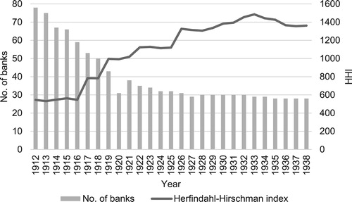
The expansion of the industry reached its peak a decade into the twentieth century, with commercial bank lending reaching close to 70 percent of GDP in the years before World War One. From the 1910s onwards, however, this expansionary phase was followed by a far-reaching consolidation of the industry, which more than halved the banking population and led to a rapid rise in market concentration. This development can be seen in Figure 1 below, which shows a Herfindahl-Hirschman index of market concentration, calculated on bank lending shares, as well as the total number of active banks for each year between 1912 and 1938. As is seen in the graph, the degree of market concentration more than doubled from the mid 1910s to the mid 1920s, while the number of active banks declined from around 80 in 1912, to a stable level of around 30 in the 1920s and 30’s. These rapid changes in market structure had both economic and political causes.

Figure 1. Herfindahl-Hirschman index of market concentration in the Swedish commercial banking industry (line) and number of active commercial banks (bars), 1912–1938. Source: Calculated from Statistiska Meddelanden, Serie E, Uppgifter om bankerna.

The fast growth of the industry during the late nineteenth century, gave rise to a significant degree of competition over depositors and borrowers. This incited banks to acquire or merge with competitors, either as a means to expand in scale or geographical scope, or in order to prevent competitors from expanding. An important contributing factor was also that the establishment of new branch offices was made subject to approval by the Bank Inspection Board in 1918, which made acquiring already existing offices an attractive alternative to new establishment (Jungerhem & Larsson, 2013, pp. 232–234). The introduction of the Bank Acts of 1903 and 1911 were no doubt also important in this regard. Inspired by the German model of universal banking, the overall objective of these acts was to safeguard market stability by tightening the banks’ liquidity and solidity requirements while at the same time improving their preconditions to increase equity and grow (Larsson & Söderberg, 2017). Solid, large banks were considered to have greater capacity to supply the domestic manufacturing industry with credit, and to be more stable than a great number of smaller banks. For this reason, capital requirements were raised in two steps, in both the 1903 and 1911 legislation (Larsson, 1993, p. 22). Due to the high level of new bank entry, which had accelerated especially after 1895, the competition over depositors and borrowers had grown increasingly fierce to levels that were considered unsound. In order to counter for this effect, the Act of 1911 also allowed banks the option to expand their activities by trading and owning shares. Although a few banks had previously been granted the right to own and trade in shares, such assets had generally only been held as collateral (Broberg & Ögren, 2019, p. 5). The Act of 1911, however, extended this right to all banks with sufficient funds, which meant that the size (volume) of the banks’ funds determined the size of its acquisitions. As banks were incited to either increase the size of their equity or merge with another bank, this encouraged extensive expansion strategies (Larsson, 1998, pp. 87–96. On the banks’ right to own and trade with shares, see Fritz, 1990).

The economic conditions that prevailed during World War One and the subsequent post-war deflationary crisis contributed to this development. During the first war years, rising foreign demand and a rapid expansion in credit volumes gave momentum to Swedish industry. Towards the end of the war, however, foreign trade began to decline, causing an increasing scarcity of goods and supplies while prices sky-rocketed; between 1914 and 1920 prices increased by 165 percent (Nygren, 1985, p. 66). In the early 1920s, prices fell and a deflationary crisis emerged. In the wake of the great number of industrial bankruptcies that followed, the banks suffered massive losses,² and set off a subsequent wave of bank mergers (Larsson, 2018, pp. 10–11).³ Between 1916 and 1922 alone, a total of 45 mergers and acquisitions were carried out within the industry; i.e. more than six per year (Wallerstedt, 1995, pp. 39–42).

According to Jungerhem and Larsson (2013, p. 234) the pressure on the financial market that followed from the deflation crisis, in combination with increasing difficulties to obtain attractive borrowers, subsequently changed the large banks’ incentives for expansion. This was reflected in the merger trend, which levelled out from the mid 1920s, but at the same time, the banks that remained grew notably larger (Larsson & Lindgren, 1989, p. 11). In 1920, the three largest banks accounted for 45 per cent of total commercial bank lending. By the early 1930s, this share had risen to almost 60 per cent. As a result, the degree of market concentration continued to rise up until 1933, and subsided somewhat thereafter. During the years when the rise in market concentration was the fastest, roughly 1917 through 1927, the concentration trend was mainly driven by large-scale banks, which expanded by acquiring numerous small – and medium-sized banks. Particularly, banks such as Handelsbanken and Skandinaviska Banken expanded rapidly during the period, becoming truly national actors after having acquired branch offices’ in several new Swedish counties, where they had not been active before. Also, a number of medium-sized banks, such as Upplands Enskilda and Sundsvalls Enskilda, markedly increased their number of branch offices through small bank acquisitions during this period (Jungerhem, 1992).

In connection with the rise in market concentration, the expense burden of commercial banks increased overall, but particularly so for the most expansionary banks. As share of gross profits, general expenses (of which the largest part were outlays for salaries) more than doubled in Handelsbanken; from 25 percent in 1912–13 to slightly above 50 percent from 1919 to 1938. The trend looked similar for all of the banks that were the most active in mergers and acquisitions during the period.⁴ This indicates that the banks which grew to dominate the national banking market during the 1920s and 1930s, experienced a concomitant deterioration in cost-efficiency. In the following, we aim to test both whether this apparent decrease in efficiency persists after controlling for the full range of bank inputs and outputs, and if so, whether this lower efficiency was connected to the consolidation of the commercial banking industry.

3. Methodology and data

Our measure of efficiency in Swedish commercial banking is based on Data Envelopment Analysis (DEA), which is a linear programming technique for identifying the best practice companies within an industry. These companies are then used as a benchmark to assign relative efficiency scores to the remaining companies, by measuring the individual deviations from best practice performance. The main advantage of DEA is that it allows for measuring efficiency using multiple inputs and multiple outputs, which is particularly useful when examining a complex business activity such as banking. To be able to examine efficiency change over time we use the DEA efficiency scores to construct a Malmquist efficiency growth index (Malmquist, 1953). The index is defined as the product of catch-up and frontier-shift, where the first term refers to the relative temporal change in efficiency of individual banks, and the second term refers to the change in the benchmark frontier (or production possibility curve) that is used to evaluate each bank. The Malmquist index thus makes it possible to examine changes in efficiency of Swedish commercial banks over time, while controlling for changes in technological development.

Figure 2 below gives a graphical depiction of the Malmquist index analysis using an example of a bank with a single input and single output (x₀, y₀) that is evaluated over two consecutive time periods. The technical efficiency of the bank in time period 1 $\left(x_0^1,y_0^1\right)$ is measured as the radial distance to the efficient frontier of period 1, or as the distance between points A and C in Figure 2 divided by the distance between points A and P. In time period 2, the catch-up component of the Malmquist index is measured as the technical efficiency of the bank in time period 2 $\left(x_0^2,y_0^2\right)$ relative to the frontier of period 2 divided by the technical efficiency of the bank in time period 1 $\left(x_0^1,y_0^1\right)$ relative to the frontier of period 1, or$\mathrm{C}\mathrm{a}\mathrm{t}\mathrm{c}\mathrm{h}\text{-}\mathrm{u}\mathrm{p}=\frac{BD}{BQ}/\frac{AC}{AP}=\frac{AP}{BQ}$

Figure 2. Graphical depiction of a data envelopment analysis over two consecutive time periods. Source: Figure adapted from figure 11.1. in Cooper et al. (2007, p. 329).

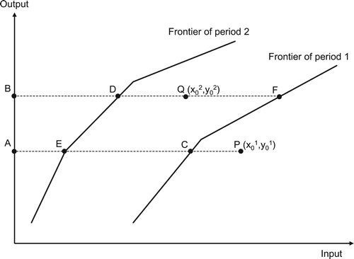
The change in the efficient frontier between time periods 1 and 2 can be measured in two ways, either from the reference point of $\left(x_0^1,y_0^1\right)$ or from the reference point of $\left(x_0^2,y_0^2\right)$. That is, either as$=\frac{AC}{AP}/\frac{AE}{AP},\mathrm{o}\mathrm{r}\mathrm{a}\mathrm{s}=\frac{BF}{BQ}/\frac{BD}{BQ}$

The frontier-shift component of the Malmquist index is therefore calculated as the geometric mean of these two possibilities, or$\mathrm{F}\mathrm{r}\mathrm{o}\mathrm{n}\mathrm{t}\mathrm{i}\mathrm{e}\mathrm{r}\text{-}\mathrm{s}\mathrm{h}\mathrm{i}\mathrm{f}\mathrm{t}=\sqrt{\left(\frac{AC}{AP}/\frac{AE}{AP}\right)\left(\frac{BF}{BQ}/\frac{BD}{BQ}\right)}=\sqrt{\left(\frac{AC}{AE}\right)\left(\frac{BF}{BD}\right)}$

The Malmquist index is then measured as the product of the catch-up and frontier-shift components. In this simple example, where the bank uses only a single input to produce a single output, the resultant DEA efficiency scores are, in essence, no different from standard partial productivity measures that have for long been widely used in economic research, such as, for instance, labour productivity or energy efficiency. The principal advantage of the DEA methodology stems, of course, from its ability to handle multiple inputs and outputs. Unlike in traditional index number approaches to this problem, the DEA approach does not require the researcher to assign appropriate weights to each input and output. Rather, DEA utilises linear programming to derive a variable weighting scheme for each unit of analysis (in our case, banks) that maximises the efficiency score of each unit relative to all other units. The resultant weighting scheme can thus be considered pareto-optimal, in the sense that none of the final weights can be altered in order to increase the efficiency score of one unit without simultaneously lowering the efficiency score of another unit.

In addition to accounting for the impact of technological change on the longitudinal development of bank efficiency, the Malmquist index can also be further decomposed into a scale effect and ‘pure’ catch-up and frontier-shift effects, in which scale effects are held constant. These decompositions enable us to distinguish between changes in bank efficiency that were due to innovation, changes that were due to the diffusion of previous innovations and changes that were due to economies or diseconomies of scale (Cooper, Seiford, & Tone, 2007).

We use a sequential reference Malmquist index, rather than the more common adjacent reference index, which means that the benchmark frontier in a given year will consist of the most efficient banks from all previous years, not just the most adjacent one. This precludes the possibility of the index exhibiting technological regress. We choose this approach, not because we hold technological regress to be impossible, but because we believe it provides a more appropriate benchmark against which to evaluate the efficiency of individual banks. We want to evaluate the technical efficiency of each bank in each year relative to the best performing production technology that was currently available. If a bank can be shown to have produced a certain volume of output using a given combination of inputs at time t, it should, theoretically, have been possible for another bank to adopt the same production technology at time t+1, regardless if, for whatever reason, this technology was not currently in use at the time.

DEA is a data-driven, non-parametric method and is, as such, considerably more flexible than regression-based alternatives, such as Stochastic Frontier Analysis (SFA). Unlike in SFA, the researcher need not specify an appropriate functional form for the relationship between inputs and outputs, or make assumptions about the distribution of inefficiency in the researched sample.⁵ The major downside of DEA is that it is not possible to draw (parametric) statistical inference. With DEA, all deviations from the efficient frontier will be interpreted as pure inefficiencies, and there is hence (1) no way to correct for sampling error, and (2) no (straightforward) way to control for non-discretionary variables; i.e. variables that may have affected the efficiency of the banks but that were not directly controlled by the banks’ management, such as, for instance, the general market conditions that prevailed during different parts of the research period. With respect to the first problem, we have chosen to analyse the entire population of Swedish commercial banks between 1912–1938, thereby eliminating the possibility of sampling error.⁶ In a second stage of our analysis, we also control for a number of important non-discretionary variables that may have affected bank efficiency during our research period using fractional regression analysis; thereby addressing the second problem.

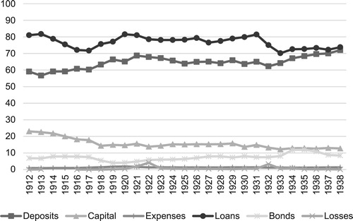
With respect to the choice of input and output variables, there are two main approaches within the banking efficiency literature; the ‘production approach’ and the ‘intermediation approach’.⁷ In the production approach banks are viewed as using physical inputs, in the form of labour and capital to produce financial services for account holders. In this approach, output is typically measured as the quantity of services provided; e.g. the number of transactions performed or documents processed. In the latter approach, banks are instead viewed primarily as intermediaries, channelling funds between savers and investors. In this approach, deposits and the interest paid to depositors are regarded as inputs along with the physical inputs used in the production approach, while output is mainly measured by the lending volume and direct investments in securities. Both approaches have their merits – as banks are both providers of financial services and financial intermediaries – but in this article, we have opted to use the intermediation approach. This choice is in part guided by practical considerations (data on, e.g. the number of transactions performed by individual banks is simply not available), but is also motivated on theoretical and historical grounds. The production approach, arguably, gives a better representation of bank activities in situations where banks supply a wide array of different financial services, each demanding a unique set of inputs, making it imperative to discriminate between different forms of service provision. In early twentieth century Swedish banking, the variety of financial services provided was, on the contrary, quite limited. For this reason, we believe that the intermediation approach renders a better model of bank activities during our research period. We use three inputs, (i) total deposits, (ii) consumption of capital⁸ and (iii) general expenses,⁹ and two outputs, (i) total loans and (ii) total holdings of bonds and shares. In order to control for the risk profile of individual banks we also include annual loan losses, which we model as an undesirable output.¹⁰ We base the choice of variables on which items were the largest in the balance sheets and hence reflect the activities of the banks, such as deposits, capital, loans, and holdings of bonds and shares. General expenses was a minor item, but is included as to reflect cost efficiency. In Figure 3 below we show the balance sheet composition including our inputs and outputs over the period. It becomes quite clear that the financial services of Swedish commercial banks were heavily focused on deposits and loans.¹¹

Figure 3. Deposits, capital, and expenses as share of total assets, and loans, bonds, and loan losses as share of total liabilities. Source: Calculated from Statistiska Meddelanden, Serie E, Uppgifter om bankerna

Lozano-Vivas and Humphrey (2002) have argued that when parts of the balance sheet are left out of the DEA analysis, efficiency scores may become biased. This is because leaving certain balance sheet items out of the analysis will yield a distorted image of what is actually produced by each bank and at what cost. Lozano-Vivas and Humphrey argue that apart from the major outputs and inputs included in the analysis, there should be two entries (one output and one input), which capture the rest of the assets and liabilities so that all of the balance sheet is included. This protects the Malmquist index from being influenced by shifts in the balance sheet composition over time. However, as Fortín and Leclerc (2007) have demonstrated, if all balance sheet items are included, all banks will, by necessity, be identified as fully efficient, due to the balance sheet restriction. All that can be shown in this case is that all banks use one unit of input to produce one unit of output, making it impossible to discriminate between banks. While we accept the problem identified by Lozano-Vivas and Humphrey, we argue that the degree of bias arising from omitted balance sheet items should be considerably smaller in our sample as compared to studies of modern-day banking as, again, the financial services offered by banks exhibited much less diversity during the early twentieth century. Furthermore, the inputs and outputs we use were consistently the most important components of the banks’ total assets and liabilities, which should further reduce the risk for such bias.

The data we use has been collected from the balance sheets and income statements of all Swedish commercial banks between 1912 and 1938. These have been accessed through Statistics Sweden’s series Uppgifter om bankerna 1912–1938, which comprises monthly data on Swedish commercial banks.¹² This data was submitted by the banks themselves, and was originally compiled and revised by the Swedish Royal Bank Inspection.¹³ For all years of our study, we have gathered data for the month of December. While yearly data does not provide the same precision as monthly, we believe that it will be temporally coherent. In total we have data for 78 individual banks in our sample, which range from a high of 65 in 1912 to a low of 27 in 1938. This is not the same as the exact number of existing commercial banks, as some have been excluded from our sample. Basis of exclusion have been: (1) where one data point was missing, which was normally the case with entries in the income statement for banks that had started their operations during the year in question. The same occasionally occurred when a bank had seized their operations (or had merged with another bank) during the fiscal year; (2) where no data was reported whatsoever. This could be the case when a bank had filed for bankruptcy during the fiscal year; the numbers for December just indicated the remaining assets and debts of the company; (3) where we had data for a bank for less than three years, as this made it impossible to calculate changes in efficiency between years; (4) finally, we have excluded one particular bank from the sample (Stockholms Industrikreditaktiebolag) as it seems to have functioned more as a mortgage institution, yielding a very high loan-to-deposit – and loan-to-capital ratio. This bank instead had two categories of inputs (for instance issuance of bonds), which were exclusive to that bank and was found for no other. Excluding this bank from the analysis of the Swedish commercial banking industry has been standard procedure in earlier research (see for instance Kock, 1932; Sjögren, 1989; Söderlund, 1978).

4. Swedish commercial bank efficiency, 1912–1938

We start by looking at the efficiency of the Swedish commercial banking sector in the year 1912, in order to establish a point of reference for the subsequent analyses. For this year, we have a total of 65 banks in our sample. We divided the banks into quartiles based on their lending volume and analysed their overall technical efficiency, returns to scale characteristics and scale efficiency. The results from this analysis can be seen in Table 1. The efficiency scores we report are all bound between 0 and 1 and can be interpreted in percentage terms. In column one, we have used a constant returns to scale (CRS) model, while in column two we have allowed for variable returns to scale (VRS). The efficiency scores reported in the second column can be regarded as ‘pure’ technical efficiency scores, as all scale effects are held constant. A measure of scale efficiency can be had by taking the ratio of the CRS and VRS scores; these ratios are reported in column three. In column four, finally, we report the most common (or mode) returns to scale characteristic within the different groups of banks.

Table 1. Swedish commercial bank efficiency in the year 1912.

Size quartile	Efficiency (CRS)	Efficiency (VRS)	Scale efficiency	RTS characteristic
Q1	0.837	0.867	0.965	Increasing
Q2	0.830	0.852	0.974	Increasing
Q3	0.868	0.912	0.952	Decreasing
Q4	0.852	0.947	0.900	Decreasing
Mean	0.847	0.894	0.947	…

Source: Calculated from Statistiska Meddelanden, Serie E, Uppgifter om bankerna.

As seen in the first column of Table 1, banks in the upper two quartiles were, on average, more efficient than banks in the bottom quartiles in 1912, but the overall differences were small. The higher efficiency of larger banks, moreover, does not seem to have been due to economies of scale. The difference in efficiency between large – and small-scale banks is only further accentuated when scale effects are held constant, as seen from the VRS efficiency scores in the second column. In column three, it can be seen that the largest scale inefficiencies were in fact found amongst the largest banks in quartile 4, with a mean scale inefficiency of around 10 per cent. Simply put, the slightly higher efficiency of large-scale banks was not due to their size, but despite of it. Our analysis does show that most of the banks in quartiles 1 and 2 were characterised by increasing returns to scale, but the average scale inefficiency within this group of banks was only around 3 per cent. All in all, this suggests that the most productive scale size for Swedish commercial banks was relatively small in 1912, situated somewhere in the range between the second and third size quartile.

Keeping these results in mind, we now turn to the analysis of changes in efficiency over time. Figure 4 below shows a Malmquist efficiency index for the Swedish commercial banking industry between the years 1912–1938. For the period as a whole, efficiency growth averaged 0.4 per cent per annum, but exhibited considerable variation between different subperiods. Between 1912 and 1917, the index hovers around the base year level, which is followed by a sharp fall between 1917 and 1920 of around 30 percentage points. Despite heavy credit losses incurred by a number of banks during the crisis of 1921–22, the index indicates an improvement in mean efficiency of around 13 per cent during these years. From 1921 up until 1927, efficiency growth in the commercial banking industry was very high compared to the rest of the period, averaging 5.3 per cent per annum. By 1927, the Malmquist index regains its base year level, indicating a return to the level of efficiency that prevailed during the period 1912–1917. From 1928 onwards, however, efficiency growth in the sector slowed down considerably, averaging only around 0.5 per cent per annum between 1928 and 1938.

Figure 4. Unweighted (solid line) and output-weighted (dotted line) Malmquist index of efficiency growth for the Swedish commercial banking industry, 1912–1938. Source: Calculated from Statistiska Meddelanden, Serie E, Uppgifter om bankerna.

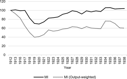
There were quite large differences in the development of the Malmquist index for different size categories of banks, with large-scale banks (quartile 4) performing considerably worse than smaller banks (quartiles 1–3). This is illustrated by the dotted line in Figure 4, which shows an output-weighted Malmquist index, where large-scale banks are given more weight. As seen in the figure, the output-weighted index shows a marked decline in efficiency taking place already from 1913. After a sharp increase in efficiency growth between 1919 and 1927, the index levels out at around 60 percent of its base year level. The efficiency growth of large-scale banks was thus clearly below the sample average, which may indicate diseconomies of scale at higher levels of output.

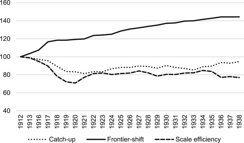
In Figure 5 below, we have disaggregated the Malmquist index into its components, i.e. catch-up-, frontier-shift – and scale efficiency growth (see method section). From this decomposition it can be seen that efficiency growth during this period was mainly the result of frontier-shift growth. That is, technological change, in the broad sense, such as changes in lending standards, reduced administration or other improvements in managerial and organisational practices, which enabled banks to provide financing at lower cost. For the period as a whole, technology growth contributed 1.6 per cent per annum to total efficiency growth. This growth in technology seems, at least initially, to have been concentrated to a smaller subset of the sample, as indicated by the negative development of the catch-up component of the Malmquist index between 1912 and 1922. For the remainder of the period, the development of the catch-up component is weakly positive, indicating that the mean distance of inefficient banks to the efficient frontier decreased somewhat between 1923 and 1938. The sharp fall in the aggregate Malmquist index between 1917 and 1920 was due to a combination of a negative catch-up effect and a marked decrease in the average scale efficiency of the sector. During the crisis of 1921–22, the average scale efficiency of the sector improved somewhat, but from 1923 onwards, it remained stable at around 80 per cent of its base year level. In aggregate terms, changes in the average scale of the banks seems thus to have had a decidedly negative impact on efficiency growth during this period.

Figure 5. Decomposition of Malmquist index for the Swedish commercial banking sector, 1912–1938 (1912 = 100). Source: Calculated from Statistiska Meddelanden, Serie E, Uppgifter om bankerna.

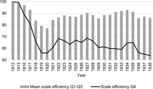
Scale inefficiencies may of course, equally well be due to banks operating below, as opposed to above, the most productive scale size (or a combination of both). In this case, however, it seems relatively clear that the increasing scale inefficiencies were mainly caused by large-scale banks operating under decreasing returns to scale. Banks in the largest size quartile had an average scale efficiency growth during the period of −3.3 per cent per annum. The corresponding average for banks in quartiles 1–3 was −0.5 per cent (see Figure 6). With exception for the 1910s, the scale efficiency growth of the smallest banks (in quartile 1) was, indeed, below that of the medium-sized banks, but was still well above that of the banks in quartile 4. The main single explanation for the slow development of the aggregate Malmquist index during this period seems thus to be that a number of large-scale banks grew too large, and came to operate under unfavourable economies of scale. Granted, this did not apply to all large-scale banks. If we look at the banks that, at one point or another during the research period, were located on the efficient frontier, this set of banks mainly consisted of medium-sized banks, but also included a small number of banks from quartile 4. But on average, large-scale banks were characterised by decreasing returns to scale and the resultant scale inefficiencies amongst the banks in size quartile 4 seems to have acted as a definite drag on efficiency growth within the commercial banking sector during this period.

Figure 6. Scale efficiency growth for banks in quartile 4 (solid line) compared to mean scale efficiency growth for banks in quartiles 1–3 (bars), 1912–1938. Source: Calculated from Statistiska Meddelanden, Serie E, Uppgifter om bankerna.

5. Market concentration and efficiency growth

The sharp fall in the aggregate Malmquist index and in the mean scale efficiency of the Swedish commercial banking industry during the late 1910s and early 1920s closely mirrors the concomitant rise in the industry’s degree of market concentration. In order to analyse more closely the connection between the industry’s market structure and its overall efficiency, we perform a series of regressions on the DEA efficiency scores that were derived from the above analysis, where we relate efficiency to a number of bank-specific and non-discretionary factors.

Performing second-stage regression analysis on DEA efficiency scores has become increasingly common practice over the past two decades, but currently, there is no broad consensus on the choice of an appropriate method. Due to the bounded nature of DEA efficiency scores, traditional linear models are in general not appropriate, though sometimes used. As DEA scores frequently take the value of unity (i.e. observations on the efficient frontier), most DEA studies generate a distribution of scores with a mass point at one. This has led to the common practice of using a two-limit tobit model, with limits at zero and one, for the second-stage regression analysis. But as Simar and Wilson (2007), Ramalho, Ramalho, and Henriques (2010) and others have pointed out, DEA efficiency scores are not actually censored, but are naturally bound between zero and one. In DEA analysis, units of observation that are on the efficient frontier (i.e. have a value of one) are identified as 100 percent efficient and are used as benchmarks for the remaining observations. The fact that it is not possible to discriminate between units on the efficient frontier does not imply censoring, but simply the theoretical impossibility of exceeding 100 percent efficiency. Moreover, as DEA scores of zero are never actually observed,¹⁴ the lower limit of the two-limit tobit model is demonstrably misspecified.

Ramalho et al. (2010) instead suggest the use of fractional regression models (or FRM’s), which were originally developed by Papke and Wooldridge (1996) as a means of dealing with naturally bounded dependent variables, such as fractions or proportions. The standard fractional logit or probit models are, however, only suitable for cross-sectional data. Using fractional regression models in a panel data setting, by simply adding cross-sectional dummies to account for unobserved heterogeneity between panel units, has been shown to introduce an incidental parameters problem, unless T is very large. We therefore use the correlated random effects probit model proposed by Papke and Wooldridge (2008) for balanced panel data sets, and employ the method outlined in Wooldridge (2018) to account for the fact that our panel is strongly unbalanced.¹⁵

We estimate a model with three bank-specific and five non-discretionary factors that can be expected to have affected bank efficiency. The bank-specific factors include dummies for bank size quartiles, a dummy for locally based banks (defined as banks which only had branch offices in one Swedish county¹⁶), and a dummy for mutual (or unlimited liability) banks. The non-discretionary factors include the growth rates of real GDP per capita, the real Swedish stock price index, real wages, the growth of the commercial banking market, and the growth of market concentration, all expressed in percentage terms.¹⁷ Our main interest in this regression is the coefficient of the last mentioned non-discretionary variable (i.e. the growth of market concentration), which we expect to have a negative sign.

The results of this analysis can be seen in Table 2. In the first and second column of Table 2, we report the results of a linear fixed effects – and a correlated random effects (or CRE) tobit model in order to illustrate that the results we get are not, primarily, driven by our choice of method. Though in the following, we only comment on the results of the CRE probit model in column three. As seen in the table, all three of the largest size quartiles of banks were, on average, more efficient than the banks in the first size quartile. The effect size of the difference diminishes from the second through the fourth size quartile however, and it is only the difference between the first and second size quartile that reaches statistical significance. This further strengthens the conclusion of the initial DEA analysis, that the Swedish commercial banking industry does not seem to have been characterised by significant economies of scale during this period; at least not above a certain size threshold. The results suggest that the most productive scale-size for Swedish commercial banks during this period was, on average, situated somewhere in the range of the second (or possibly third) size quartile. Our results also show that locally based banks were, on average, considerably more efficient than banks that had branch offices in multiple counties. This result is in line with Söderlund (1978), whom argued that the intense competition for deposits during the 1910s and 1920s led to the establishment of a growing number of unprofitable branch offices (Söderlund, 1978, p. 388). It is also consistent with a recent strand of the banking performance literature, which has argued that the effectiveness of screening procedures tends to deteriorate with the distance between bank and borrower, resulting in a larger incidence of non-performing loans (Deng & Elyasiani, 2008; Goetz, Laeven, & Levine, 2013; Liberti & Mian, 2009). The coefficient for the third bank-specific factor, unlimited liability (or mutual) banking, is also positive and statistically significant. This result may in part be due to the fact that our research period covers two Swedish financial crises and was characterised by a secular decline in stock prices, which may have presented join-stock banks with greater difficulties than mutual banking companies. Moreover, the Bank Act of 1934 prohibited unlimited liability banking, which means that a number of mutual banks were forced to adopt the joint-stock company form from 1935 onwards. All of the targeted mutual banks (of which there were seven in 1934) were characterised by below average efficiency growth during 1935–1938, which in turn may have had less to do with the joint-stock company form in itself, and more to do with the fact that these companies were forced to adopt it.

Table 2. Regression estimates of the impact of bank-specific and non-discretionary factors on Swedish commercial bank efficiency, 1913–1938.

	OLS FE	CRE Tobit	CRE Probit
Quartile 2	6.13*	6.08**	4.49*
	(2.42)	(0.23)	(2.28)
Quartile 3	7.79†	8.18*	3.91
	(3.97)	(3.34)	(3.74)
Quartile 4	5.99	6.3	2.89
	(5.31)	(3.91)	(4.57)
Local	21.38**	22.03**	10.22*
	(4.21)	(3.33)	(4.10)
Unlimited liability	4.88	4.95*	5.95*
	(3.76)	(2.25)	(2.34)
Real GDP	0.02	0.04	0.18
	(0.12)	(0.15)	(0.16)
Real stock prices	0.16**	0.16**	0.17**
	(0.04)	(0.04)	(0.03)
Real wages	−0.43**	−0.43**	−0.48**
	(0.12)	(0.15)	(0.13)
Market size	0.26**	0.26**	0.29**
	(0.07)	(0.08)	(0.09)
Market concentration	−0.12**	−0.13**	−0.09*
	(0.03)	(0.04)	(0.04)
N	813	813	813
R^2	0.13	…	…
Log(pseudo)likelihood	…	479.80	−531.32

Note: Robust standard errors in parenthesis. The coefficients reported in the second and third column are the average partial effects. **, * and † denote statistical significance at the 1%, 5% and 10% level respectively.

All of the coefficients of the non-discretionary factors reported in Table 2 are significant (with exception for the growth in real GDP per capita), and have relatively large effect sizes. A one percent fall in real stock prices is estimated to have reduced commercial bank efficiency by 0.17 percent on average, while a one percent rise in real wages reduced efficiency by 0.48 percent. Judging from these coefficients, it seems clear that the rapid fall in the Malmquist index during the early part of the research period was only partly due to the adoption of inefficient banking practices, as real stock prices fell by 75 per cent, and real wages increased by 17 percent during this period. The effect of falling stock prices and rising real wages was, however, partly offset by the coincident growth of the Swedish commercial banking market. After controlling for these effects, a one percent growth in market concentration is still estimated to have reduced efficiency in the banking population by, on average, 0.09 percent. This may sound like a small effect size, but considering that the level of market concentration in the industry increased by 250 percent between 1912 and 1938, this translates to a 22.5 percent decrease in efficiency, all else held equal.

After having established that the growth in market concentration that took place during the period was detrimental for efficiency, we next turn to the question of the impact of bank mergers. If market concentration was negative for efficiency, we should find that bank mergers, on average, reduced the efficiency of the merged banks. In this sense, we view an analysis of bank mergers as a kind of robustness check for the results in Table 2. The hypothesis that bank mergers were associated with a decrease in efficiency can be motivated on several grounds. First of all, large-scale banking may have been characterised by decreasing returns to scale, as our previous analysis seems to suggest. The vast majority of mergers that took place within the commercial banking industry during this period involved larger banks (banks in the third and fourth size quartile) acquiring smaller banks (in the first and second size quartile). If banks in the upper size quartiles operated under disadvantageous economies of scale, many mergers may have contributed to exacerbating scale-inefficiencies. Secondly, several of the mergers involved locally based banks that acquired banks with branch offices in outside counties. Many mergers may consequently also have decreased the efficiency of the merged banks by introducing greater difficulties in the screening and monitoring of loans (Goetz et al., 2013), or if the acquisition of new branch offices was not followed by adequate rationalisation efforts (Söderlund, 1978, pp. 48–50).

In the first column of Table 3 below, we re-estimate the previous CRE probit model from Table 2 with the addition of a dummy variable coding for merged banks, as well as three lags of this variable. Most of the coefficients from the previous model remain more or less unchanged, with exception for the coefficient for banks in size quartile three, which now reaches significance at the ten percent level, and the coefficient for locally based banks, which decreases noticeably in effect size. The coefficient of the dummy coding for merged banks is −9.06 and is significant at the one percent level, indicating that mergers on average reduced the efficiency of merged banks in the order of nine percent. All three lags of this variable are also highly significant, and have similar effect sizes.

Table 3. Regression estimates of the impact of bank mergers, and estimates of the probability of a bank being targeted for acquisition, 1913–1938.

	CRE Probit	CPhM
Efficiency score	…	5.99*
	…	(4.98)
Quartile 2	4.54**	0.72
	(1.68)	(0.27)
Quartile 3	4.68†	2.35†
	(2.41)	(1.14)
Quartile 4	3.45	0.60
	(3.39)	(0.43)
Local	7.69**	1.31
	(2.61)	(0.71)
Unlimited liability	6.66**	0.23**
	(2.13)	(0.12)
Real GDP	0.17	0.85*
	(0.15)	(0.07)
Real stock prices	0.16**	1.03†
	(0.03)	(0.02)
Real wages	−0.47**	1.06
	(0.13)	(0.09)
Market size	0.32**	1
	(0.09)	(0.05)
Market concentration	−0.08*	1
	(0.03)	(0.01)
Merger	−9.06**	…
	(1.83)	…
Mergert+1	−8.19**	…
	(2.76)	…
Mergert+2	−8.48**	…
	(1.75)	…
Mergert+3	−7.08**	…
	(1.85)	…
N	813	813
Log pseudolikelihood	−529.63	−145.56

Note: Robust standard errors in parenthesis. The coefficients reported in the first column are the average partial effects, while the coefficients in the second column are odds ratios. **, * and † denote statistical significance at the 1%, 5% and 10% level respectively.

The negative effect we find for mergers could, of course, be due to that the average merger target was characterised by low efficiency. We know, for instance, from previous research that a number of small banks were forced to merge with larger banks after taking on heavy loan losses during the 1920s crisis. We can identify three such cases in our data: the mergers of Köpmannabanken and Affärsbanken with Södermanlands enskilda bank in 1921 and 1922 respectively, and the merger of Nylands folkbank with Sundsvalls enskilda bank in 1921. If banks that were targeted for mergers were, on average, poorly managed, or banks in distress, the negative outcome of the mergers could simply be an artefact of the merger targets acting as a drag on the efficiency of the acquiring banks. In column two of Table 3 we therefore estimate a Cox proportional hazards model of the probability of a bank being targeted for acquisition during our research period. As seen in the table, efficient banks were, quite to the contrary, much more likely to be targeted for acquisition than inefficient banks.¹⁸ In fact, in the vast majority of merger cases, the acquired bank had an efficiency score that was greater than that of the acquirer in the year prior to the merger. Moreover, in 70 percent (or 25 out of 36) of the mergers where we have data on the efficiency of targeted banks in the year prior the merger, these banks had an efficiency score that was above the industry average. Consequently, the negative outcome of the mergers seems to have had less to do with the merger targets, and more to do with the acquirers.

As seen in Table 3, controlling for the effect of mergers does not render the market concentration variable insignificant. The coefficient for the growth in market concentration remains significant at the 5 percent level also in this model and is only marginally reduced in effect size. This is because controlling for the effect of mergers on the efficiency of merged banks actually only captures part of the true effect of mergers on the industry’s average efficiency. As most merger targets were relatively efficient, this means that mergers had an adverse effect on industry average efficiency not only through their direct impact on the efficiency of the merged banks, but also indirectly, in that the mergers resulted in the exit of above average efficient banks from the market.

Our results thus strongly suggest that the wave of bank mergers that took place during this period, and the concomitant rise in market concentration, exerted a negative impact on the industry’s average efficiency. Granted, the period we study is not exempt from confounding factors, as it encompasses both World War One and two major banking crises. Even though we control for a number of non-discretionary factors that may have affected bank efficiency, one might still suspect that the extraordinary conditions that prevailed during the early 1920s and 1930s is what is driving our results. Furthermore, it would also not be unreasonable to suppose that possible gains from the mergers may have taken more than three years to materialise. In order to test the robustness of our results, we therefore tried adding seven additional lags to the merger variable, experimented with dropping the crisis years (1920–22 and 1929–32) from our sample, and allowed for bank-level clustering of standard errors. None of these alterations did, however, change the estimates of the impact of market concentration and bank mergers in any meaningful way (see the appendix for details).

6. Conclusions

In this article we have examined the technical efficiency of Swedish commercial banks between the years 1912 and 1938, using data envelopment analysis (DEA). The main objective of the article has been to examine the link between changes in the commercial banking industry’s market structure and industry average efficiency. During our research period, the Swedish commercial banking industry underwent a rapid consolidation phase, which more than halved the banking population, which made this an ideal case to study the impact of market concentration on bank efficiency. By regressing the derived DEA efficiency scores on a set of bank-specific and non-discretionary determinants of efficiency, we were able to isolate the impact of the growth in market concentration on industry average efficiency, while controlling for observed (and unobserved) heterogeneity between banks, and factors that were outside the control of the banks’ management.

We found that the growth in market concentration had a distinct negative impact on efficiency. Our estimates suggest that, all else held equal, increased market concentration alone reduced industry average efficiency by over 20 percent during or research period. Consistent with this finding, we also found that bank mergers, on average, reduced the efficiency of merged banks by almost ten percent. The intense merger activity of the period almost certainly had an even broader impact on industry average efficiency, as the vast majority of targeted banks had above average efficiency scores in the year prior to the merger. In fact, the level of efficiency was shown to have been one of the most important determinants of the probability of a bank being targeted for acquisition during the period.

Our analysis further suggests that the negative relationship between market concentration and efficiency was due to the fact that the most productive scale-size of Swedish commercial banks was much smaller during this period, than what has commonly been assumed in previous research. In 1912, most of the banks in the upper two size quartiles operated under decreasing returns to scale. The wave of mergers that followed, which saw large-scale banks acquiring small – and medium-scale banks en masse, therefore tended to exacerbate already existing scale inefficiencies. Scale-efficiency growth within the largest size quartile was, consequently, well below the industry average for the period as a whole. Our analysis also shows that locally based banks, i.e. banks which only had branch offices in one Swedish county, were, on average, considerably more efficient than banks with a wider geographical reach. As many of the mergers that took place during the period involved locally based banks that acquired banks with branch offices in outside counties as well as, more generally, non-locally based banks, which further expanded their geographical reach as a result of the mergers, the negative relationship between bank mergers and overall efficiency likely had many causes. For instance, (i) granting large – as opposed to small-scale credits may have required disproportionately larger input volumes, (ii) a wider geographical network of branch offices may have entailed high fixed costs, that were not offset by rationalisation efforts, (iii) locally based banks may have been better equipped to assess loan risk, due to superior local knowledge and better managed relationships with debtors, or (iiii) commercial banks may, more generally, have been characterised by much greater complexity in management above a certain size (or scope) threshold.

What sets this case apart from most cases that have been studied in the banking efficiency literature, is that it deals with a newly industrialised economy with a relatively segmented banking industry that underwent rapid and far-reaching consolidation. The fact that our results differ from the standard results in the literature could thus, plausibly, be taken to indicate that the impact of market concentration on bank efficiency may be very different in developed and developing banking markets. Recent research from contemporary emerging economies indeed suggest that this may be the case, though the evidence is currently mixed. As a suggestion for future research in this field, more attention should be paid to the initial level of bank market concentration, and to the actual magnitude of changes in concentration, as this may have important implications for its impact on bank performance. With this article, we provide a way to move forward with this type of efficiency analysis on historical material.

As a final note, it should perhaps be emphasised that the fact that market concentration was detrimental for the efficiency of Swedish commercial banking in the 1910s through the 1930s does not, necessarily, mean that the consolidation of the industry was detrimental for the wider Swedish economy. The large industrial – and above all infrastructure projects that were launched in Sweden during this period presupposed the existence of large-scale intermediaries, with the capacity to handle large financial flows. It does seem however, that the ability of the Swedish economy to fund large-scale projects came at the cost of increased deadweight losses.

Acknowledgements

We thank the three anonymous reviewers who helped us to improve the article, as well as friends and colleagues on panel 020202 of the 43rd Annual Economic and Business History Society Conference (University of Jyväskylä), and participants of the UCBH-seminar (Uppsala University) – especially Professor Mats Larsson – for valuable comments, and finally to Jan Wallanders och Tom Hedelius Stiftelse for funding the research project (P15-0064, ‘Financial market regimes, bank efficiency and economic growth in Sweden, 1866-2016’)

Disclosure statement

No potential conflict of interest was reported by the author(s).

Additional information

Funding

This work was supported by Jan Wallanders och Tom Hedelius Stiftelse samt Tore Browaldhs Stiftelse: [grant number P15-0064].

Notes

1 Recent research on contemporary emerging economies suggest this may be the case. See, for instance, Ariss (2010, pp. 765–775); Zhang, Jiang, Qu, Wang (2013, pp. 149–157).

2 The loan losses amounted to around 2.5 per cent of the total lending volume in 1921 and over 5 per cent in 1922. The only other year during the period, which came close to these figures was 1932, following the collapse of the Krueger financial empire. It should of course be noted, that in both of these crises, there were considerable differences between the banks in terms of the magnitude of loan losses.

3 As share of total capital, the banks’ average aggregate losses were nine percent in 1922, but there were large differences between banks.

4 For instance, Göteborgs bank, Mälareprovinsernas bank, Skandinaviska Banken and Södermanlands Enskilda.

5 It should be noted, however, that when DEA and SFA have been compared they have often been shown to yield results with small to no differences between them. See for instance Cullinane et al. (2006).

6 As we analyze the entire target population, the efficiency scores we report are, in other words, not estimates but population values for our focus variable.

7 For an extended discussion of the merits of each approach, see Berger and Humphrey (1997).

8 It is common practice in banking efficiency studies to include bank capital as an input. However, when capital is consumed by a bank to cover operating losses this effectively reduces this input, making the bank appear more efficient. For this reason, we only include actual consumption of capital as an input. If the volume of a bank’s total capital remained unchanged between years this input was thus recorded as zero.

9 The general expenses included outlays for salaries for employees (the single largest item), taxes, costs for offices and equipment, deposits to pension accounts for upper management, and other minor expenses not specified.

10 Loan losses are unfortunately not available in our data source for the years 1914 and 1915. We have therefore dropped both these years from our analysis.

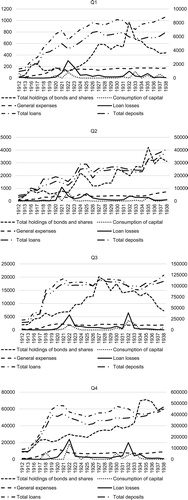
11 In the appendix, we show the development of each input and output used in the analyses for the different size quartiles of the banking population. There were some differences between banks’ balance sheet compositions, but apart from one example which we have excluded from the analysis, Stockholms Industrikreditaktiebolag, these differences were small.

12 The data is accessible at https://www.ucbh.uu.se/research/databases/. Swedish Commercial Bank Database, 1866–1994, version 2.0 (Henric Häggqvist, Viktor Persarvet, Peter Hedberg, Lars Karlsson, Mats Larsson).

13 Wendschlag (2012), among others, has shown that during the time which is in our scope, new legislation made it increasingly difficult for Swedish banks to evade supervision from the authorities. Swedish banks reported monthly about their activities to the Swedish Bank Inspection, under threat of sanctions, and the Bank Inspection regularly made on-site visits to the banks. Therefore, these official records are commonly regarded as reliable by scholars.

14 As long as an observational unit produces at least some output the DEA score assigned to that unit can only approximate zero, but can never be zero.

15 The estimation was performed in Stata using a user-written command called fhetprob, developed by Bluhm (2013).

16 When constructing this variable, we used the current Swedish administrative division with 21 counties. In a few cases, there were banks that only had a single branch office outside its principal county. When this office was located close to the border of the principal county, we coded the bank as locally based.

17 Data on real GDP per capita are from Table 5 in Schön and Krantz (2012). Data on stock prices are from Waldenström (2014), Table A6.4. Data on real wages are from Edvinsson (2005). We have used data on wages and salaries (including social benefits) of employees in the sector “Other private services”, divided by the number of employees in said sector and deflated by the Swedish CPI. The market size and market concentration variables finally, have been constructed using data from Statistiska Meddelanden, Serie E, Uppgifter om bankerna, 1912–1938. Market growth is measured as the percentage change in the real aggregate loan volume, while the growth of market concentration is measured as the percentage change in the Herfindahl–Hirschman index,

18 As the predictor variable is measured on the unit interval the coefficient 5.99 should, in this case, be interpreted as showing that a fully efficient bank (with efficiency score = 1) was ∼ 6 times as likely to be targeted for acquisition, as compared to a fully inefficient bank (with efficiency score = 0). Consequently, a bank with an efficiency score of, for example, 0.8 would thus have been around 60 percent more likely to be acquired than a bank with an efficiency score of 0.7 (as (0.8–0.7)*5,99)*100 = ∼ 60). As seen in the table, mutual banks were only around ¼ as likely to be acquired as joint-stock banks, and years with fast real GDP per capita growth saw fewer mergers (a one percent increase in the growth rate of real GDP per capita is estimated to have reduced the likelihood of mergers by 15 percent).

Appendix

Table A1 below shows regression results for four alternative model specifications of the impact of market concentration and mergers on commercial bank efficiency. In column one we have included seven additional lags of the merger variable, and in the second column we estimate the same model but allow for bank-level clustering of standard errors. As seen in the table, both models confirm that bank mergers exerted a negative impact on the efficiency of merged banks up to seven years after the merger, and do not affect the coefficient of the market concentration variable. In column three we have omitted the crisis years (1920–22 and 1929–32), in order to ensure that our results are not driven by the extraordinary circumstances that prevailed during these years, and in column four we again estimate the same model with standard errors clustered at the bank-level. The effect size of the merger variable and its lags becomes somewhat smaller in column 3 and 4, but the interpretation remains the same. The coefficient of the market concentration variable, on the other hand, increases from −0.08 to −0.21. This most likely reflects the fact that several large commercial banks underwent reconstruction during the two crises periods, which improved their efficiency scores. The only important change in table A.1. as compared to the results reported in Tables 2 and 3, is that the coefficient of the local banking variable seizes to be significant in column four (and is only significant at the ten percent level in column three). This may indicate that it was mainly during the crises years that local banks outperformed banks that were active in multiple counties.

Table A1. Robustness tests.

	(1)	(2)	(3)	(4)
Quartile 2	4.24**	4.24**	5.73**	5.73**
	(1.40)	(1.50)	(2.10)	(1.94)
Quartile 3	4.95*	4.95**	8.35*	8.35*
	(2.10)	(1.78)	(3.58)	(3.78)
Quartile 4	5.39	5.39	6.42	6.42
	(3.50)	(4.06)	(4.46)	(4.46)
Local	5.80**	5.80**	8.36†	8.36
	(2.09)	(2.14)	(4.42)	(5.13)
Unlimited liability	7.41**	7.41†	6.54**	6.54†
	(2.33)	(4.07)	(2.04)	(3.52)
Real GDP	0.09	0.09	−0.13	−0.13
	(0.12)	(0.08)	(0.23)	(0.18)
Real stock prices	0.17**	0.17**	0.22**	0.22**
	(0.03)	(0.03)	(0.04)	(0.03)
Real wages	−0.38**	−0.38**	0.35	0.35
	(0.12)	(0.10)	(0.27)	(0.22)
Market size	0.25**	0.25**	0.67**	0.67**
	(0.09)	(0.08)	(0.12)	(0.10)
Market concentration	−0.08**	−0.08**	−0.21**	−0.21**
	(0.03)	(0.02)	(0.05)	(0.04)
Merger	−11.89**	−11.89**	−10.71**	−10.71**
	(2.05)	(2.82)	(2.63)	(3.19)
Mergert+1	−12.04**	−12.04**	−7.26*	−7.26*
	(2.48)	(3.12)	(3.29)	(3.69)
Mergert+2	−12.83**	−12.83**	−9.97**	−9.97**
	(1.95)	(2.38)	(2.65)	(2.82)
Mergert+3	−13.40**	−13.40**	−9.20**	−9.20**
	(2.52)	(3.51)	(2.35)	(2.69)
Mergert+4	−13.44**	−13.44**	−10.07**	−10.07**
	(2.18)	(2.98)	(2.57)	(3.10)
Mergert+5	−14.10**	−14.10**	−10.18*	−10.18*
	(3.56)	(5.11)	(3.98)	(4.94)
Mergert+6	−12.06**	−12.06*	−8.57*	−8.57†
	(3.46)	(4.85)	(4.27)	(4.94)
Mergert+7	−10.72**	−10.72**	−10.10**	−10.10*
	(3.76)	(3.43)	(2.99)	(4.04)
Mergert+8	−5.75	−5.75	−5.57	−5.57
	(3.82)	(4.28)	(5.60)	(6.95)
Mergert+9	−6.05	−6.05	−4.79	−4.79
	(4.76)	(4.94)	(5.58)	(5.79)
Mergert+10	−8.53†	−8.53	−10.66**	−10.66**
	(4.93)	(5.21)	(3.38)	(2.77)
N	813	813	588	588
Log pseudolikelihood	−528.17	−528.17	−373.74	−373.74

Note: (Cluster-)Robust standard errors in parenthesis. The coefficients reported are the average partial effects. **, * and † denote statistical significance at the 1%, 5% and 10% level respectively.

Figure A1. Inputs and outputs used in the DEA analyses in section 4 for different size categories of banks. Total loans and total deposits (right y-axis), total holdings of bonds and shares, general expenses, consumption of capital and loan losses (left y-axis). Source: Calculated from Statistiska Meddelanden, Serie E, Uppgifter om bankerna.

References

- Allen, F., & Gale, D. (2000). Comparing financial systems. Cambridge, MA: MIT Press.
- Ariss, R. T. (2010). On the implications of market power in banking: Evidence from developing countries. Journal of Banking and Finance, 34(4), 765–775. doi: 10.1016/j.jbankfin.2009.09.004
- Bain, J. S. (1956). Barriers to new competition. Cambridge, MA: Harvard University Press.
- Beck, T., Demirguc-Kunt, A., & Levine, R. (2006). Bank concentration, competition, and crises: First results. Journal of Banking and Finance, 30(5), 1581–1603. doi: 10.1016/j.jbankfin.2005.05.010
- Berg, S. A., Førsund, F. R., & Jansen, E. S. (1992). Malmquist Indices of productivity growth during the Deregulation of Norwegian banking, 1980-89. The Scandinavian Journal of Economics, 94, 211–228. doi: 10.2307/3440261
- Berger, A. N., et al. (2002). Does Function follow organizational form? evidence from the lending practices of large and small banks. NBER Working Paper Series No. 8752.
- Berger, A. N., & Hannan, T. H. (1998). The efficiency cost of market power in the banking industry: A test of the ‘quiet life’ and related Hypotheses. The Review of Economics and Statistics, 80(3), 454–465. doi: 10.1162/003465398557555
- Berger, A. N., & Humphrey, D. B. (1997). Efficiency of financial Institutions: International Survey and Directions for future research. European Journal of Operational Research, 98(2), 175–212. doi: 10.1016/S0377-2217(96)00342-6
- Bluhm, R. (2013). fhetprob: A fast QMLE stata routine for fractional response models with multiplicative heteroskedasticity, UNU-MERIT Working Paper. Maastricht: United Nations University.
- Broberg, O., & Ögren, A. (2019). Names, shares and mortgages: The formalisation of Swedish commercial bank lending, 1870-1938. Financial History Review, 26(1), 81–108. doi: 10.1017/S0968565019000015
- Carter, D. A., & McNulty, J. E. (2005). Deregulation, technological change, and the business-lending performance of large and small banks. Journal of Banking and Finance, 29(5), 1113–1130. doi: 10.1016/j.jbankfin.2004.05.033
- Cooper, W. W., Seiford, L. M., & Tone, K. (2007). Data envelopment analysis. Boston, MA: Kluwer Academic.
- Cottrell, P. L., Lindgren, H., & Teichova, A. (1992). European banking and industry between the wars: A review of bank-industry relations. Leicester: Leicester University Press.
- Cullinane, K., et al. (2006). The technical efficiency of container ports: Comparing data envelopment analysis and stochastic frontier analysis. Transportation Research Part A: Policy and Practice, 40(4), 354–374.
- Demirguç-Kunt, A., & Levine, R. (2000). Bank concentration: Cross-country evidence, World Bank Working Paper Series No. 27828.
- Deng, S., & Elyasiani, E. (2008). Geographic diversification, bank Holding company value, and risk. Journal of Money, Credit and Banking, 40(6), 1217–1238. doi: 10.1111/j.1538-4616.2008.00154.x
- DeYoung, R. (1997). Bank mergers, X-efficiency, and the market for corporate control. Managerial Finance, 23(1), 32–47. doi: 10.1108/eb018600
- Du, K., & Sim, N. (2016). Mergers, acquisitions, and bank efficiency: Cross-country evidence from emerging markets. Research in International Business and Finance, 36, 499–510. doi: 10.1016/j.ribaf.2015.10.005
- Edvinsson, R. (2005). Growth, accumulation, crises: With new macroeconomic data for Sweden. Stockholm: Stockholm University.
- Fortín, M., & Leclerc, A. (2007). Should we abandon the intermediation approach for analyzing banking performance? GRÉDI Working paper 07-01.
- Fritz, S. (1990). Affärsbankernas aktieförvärvsrätt under 1900-talets första decennier. Stockholm: Almqvist and Wiksell International.
- Gale, B. T., & Branch, B. S. (1982). Branch, “concentration versus market share: Which determines performance and why does it matter? The Antitrust Bulletin, 27(1), 83–103.
- Glete, J. (1987). Ägande och industriell omvandling: ägargrupper, skogsindustri, verkstadsindustri 1850-1950. Stockholm: SNS Förlag.
- Goetz, M. R., Laeven, L., & Levine, R. (2013). Identifying the valuation effects and agency costs of corporate diversification: Evidence from the geographic diversification of U.S. banks. The Review of Financial Studies, 26(7), 1787–1823. doi: 10.1093/rfs/hht021
- Jungerhem, S. (1992). Banker i fusion. Uppsala: Uppsala University.
- Jungerhem, S., & Larsson, M. (2013). Bank mergers in Sweden: The interplay between bank owners, bank management, and the state, 1910–2009. In H. Andersson, V. Havila, & F. Nilsson (Eds.), Mergers and acquisitions: The critical role of stakeholders, 224–246. New York: Routledge.
- Kock, K. (1932). Svenskt bankväsen i våra dagar. Stockholm: Kooperativa förbundets bokförlag.
- Larsson, M. (1993). Aktörer, marknader och regleringar – Sveriges finansiella system under 1900-talet, Uppsala Papers in financial History No 1. Uppsala: Uppsala University.
- Larsson, M. (1998). Staten och kapitalet – det svenska finansiella systemet under 1900-talet. Stockholm: SNS Förlag.
- Larsson, M. (2018). Krig, kriser och tillväxt: 1914-1945. Stockholm: Dialogos.
- Larsson, M., & Lindgren, H. (1989). Risktagandets gränser. Utvecklingen av det svenska bankväsendet 1850-1980, Uppsala Papers in Economic History. Basic Reading No 6. Uppsala: Uppsala University.
- Larsson, M., & Lönnborg, M. (2014). Finanskriser i Sverige. Lund: Studentlitteratur.
- Larsson, M., & Söderberg, G. (2017). Finance and the welfare state. Banking development and regulatory principles in Sweden, 1900-2015. Basingstoke: Palgrave Macmillan.
- Liberti, J. M., & Mian, A. R. (2009). Estimating the effects of hierarchies on information use. The Review of Financial Studies, 22(10), 4057–4090. doi: 10.1093/rfs/hhn118
- Lindgren, H. (1993). Finanssektorn och dess aktörer. In B. Furuhagen (Ed.), Äventyret Sverige (pp. 241–263). Stockholm: Utbildningsradion.
- Lozano-Vivas, A., & Humphrey, D. B. (2002). Bias in Malmquist index and cost function productivity measurement in banking. International Journal of Production Economics, 76(2), 177–188. doi: 10.1016/S0925-5273(01)00162-1
- Malmquist, S. (1953). Index numbers and indifference surfaces. Trabajos de Estadistica, 4(2), 209–242. doi: 10.1007/BF03006863
- Maudos, J., & Fernandez de Guevara, J. (2007). The cost of market power in banking: Social welfare loss vs. cost efficiency. Journal of Banking and Finance, 31(7), 2103–2125. doi: 10.1016/j.jbankfin.2006.10.028
- Molyneux, P., & Forbes, W. (1995). Market structure and performance in European banking. Applied Economics, 27(2), 155–159. doi: 10.1080/00036849500000018
- Neumark, D., & Sharpe, S. A. (1992). Market structure and the nature of price rigidity: Evidence from the market for consumer deposits. The Quarterly Journal of Economics, 107(2), 657–680. doi: 10.2307/2118485
- Nygren, I. (1983). Transformation of bank structures in the industrial period. The case of Sweden, 1820-1913. Journal of European Economic History, 12, 29–68.
- Nygren, I. (1985). Från Stockholms Banco till Citibank. Svensk kreditmarknad under 325 år. Malmö: Liber Förlag.
- Ögren, A. (2010). The Swedish financial revolution: An in-depth study. New York: Palgrave Macmillan.
- Papke, L., E., & Wooldridge, J., M. (1996). Econometric methods for fractional response variables with an application to 401(k) plan participation rates. Journal of Applied Econometrics, 11(6), 619–632. doi: 10.1002/(SICI)1099-1255(199611)11:6<619::AID-JAE418>3.0.CO;2-1
- Papke, L. E., & Wooldridge, J. M. (2008). Panel data methods for fractional response variables with an application to test pass rates. Journal of Econometrics, 145(1-2), 121–133. doi: 10.1016/j.jeconom.2008.05.009
- Pilloff, S. J. (1996). Performance changes and shareholder wealth creation associated with mergers of publicly traded banking institutions. Journal of Money, Credit and Banking, 28(3), 294–310. doi: 10.2307/2077976
- Ramalho, E. A., Ramalho, J. S., & Henriques, P. D. (2010). Fractional regression models for second stage DEA efficiency analysis. Journal of Productivity Analysis, 34(3), 239–255. doi: 10.1007/s11123-010-0184-0
- Schön, L., & Krantz, O. (2012). Swedish historical national accounts 1560-2010, Lund Papers in Economic History 123. Lund: Lund University.
- Simar, L., & Wilson, P. W. (2007). Estimation and inference in two-stage, semi-parametric models of production processes. Journal of Econometrics, 136(1), 31–64. doi: 10.1016/j.jeconom.2005.07.009
- Sjögren, S. (1989). Kreditförbindelser under mellankrigstiden: krediter i svenska affärsbanker 1924-1944 fördelade på ekonomiska sektorer och regioner, Uppsala papers in economic history 21. Uppsala: Uppsala University.
- Söderlund, E. (1978). Skandinaviska banken i det svenska bankväsendets historia, 1914-1939. Uppsala: Almqvist & Wiksell.
- Statistics Sweden. Statistiska Meddelanden, Serie E, Uppgifter om bankerna, 1912-1938.
- Waldenström, D. (2014). Swedish stock and bond returns, 1856-2012. In R. Edvinsson, T. Jacobson, & D. Waldenström (Eds.), Historical monetary and financial statistics for Sweden, volume II: House prices, stock returns, national Accounts, and the Riksbank balance sheet, 1620-2012, 223–292. Stockholm: Ekerlids förlag.
- Wallerstedt, E. (1995). Finansiärers fusioner. De svenska affärsbankernas rötter 1830-1993, Studia Oeconomiae Negotiorum 37. Uppsala: Uppsala University.
- Wendschlag, M. (2012). Theoretical and empirical accounts of Swedish financial supervision in the twentieth century. Linköping: Linköping University.
- Wooldridge, J. M. (2018). Correlated random effects models with unbalanced panels. Journal of Econometrics, 211(1), 137–150. doi: 10.1016/j.jeconom.2018.12.010
- Zhang, J., Jiang, C., Qu, B., & Weng, P. (2013). Market concentration, risk-taking, and bank performance: Evidence from emerging economies. International Review of Financial Analysis, 30(C), 149–157. doi: 10.1016/j.irfa.2013.07.016
Appendix
below shows regression results for four alternative model specifications of the impact of market concentration and mergers on commercial bank efficiency. In column one we have included seven additional lags of the merger variable, and in the second column we estimate the same model but allow for bank-level clustering of standard errors. As seen in the table, both models confirm that bank mergers exerted a negative impact on the efficiency of merged banks up to seven years after the merger, and do not affect the coefficient of the market concentration variable. In column three we have omitted the crisis years (1920–22 and 1929–32), in order to ensure that our results are not driven by the extraordinary circumstances that prevailed during these years, and in column four we again estimate the same model with standard errors clustered at the bank-level. The effect size of the merger variable and its lags becomes somewhat smaller in column 3 and 4, but the interpretation remains the same. The coefficient of the market concentration variable, on the other hand, increases from −0.08 to −0.21. This most likely reflects the fact that several large commercial banks underwent reconstruction during the two crises periods, which improved their efficiency scores. The only important change in table A.1. as compared to the results reported in and , is that the coefficient of the local banking variable seizes to be significant in column four (and is only significant at the ten percent level in column three). This may indicate that it was mainly during the crises years that local banks outperformed banks that were active in multiple counties.