The quest for economic stability: a study on Swedish stabilisation policies 1873–2019

ABSTRACT

This paper explores the evolution of Swedish stabilisation policies through six policy regimes between 1873 and 2019. We focus on discretionary policy decisions by estimating policy shocks using a SVAR model. Through these shocks, we explore how stabilisation policies have evolved over time and how policymakers responded to key economic events such as financial crises and wars. Our results show three key results (i) policies are often a source of destabilisation rather than stabilisation, (ii) regimes are designed for a specific time and ends when economic circumstances change, and (iii) fixed exchange rates worsen the economic effects of financial crises.

KEYWORDS:

• monetary policy
• fiscal policy
• policy shocks
• stabilisation policies
• financial crisis

SUBJECT CLASSIFICATION CODES:

• E42
• E43
• E52
• E58
• E62
• E65

1. Introduction

There is a never-ending quest for a stable economy with full employment and low inflation. Economists have suggested, and policymakers have experimented with, different fiscal and monetary policy regimes since at least the beginning of the industrial revolution. Most regimes have been successful for a time, but none of them have stood the test of time. In this paper, we explore Swedish stabilisation policies from the introduction of the gold standard in 1873 until 2019. We explore the evolution of stabilisation policies over time, how different institutional setups affected the policies adopted, and how policymakers responded to key economic events such as financial crises and wars.

Sweden is an interesting case. Having enjoyed peace for more than 200 years (the last war ended in 1814), institutions and policies have evolved over time, without any major interruption through wars or revolutions. Policymakers have often been early adopters of new economic ideas. For example, Sweden tried price level targeting based on Wicksell’s (1898) norm during the 1930s. Keynesian-type fiscal stabilisation policies were introduced in the early 1930s as a response to the Great Depression (Berg & Jonung, 1999; Jonung, 1979). Sweden experimented with a ‘third way’ in the 1980s as an alternative to both the increasingly dominant monetarist and supply-side ideas and traditional Keynesian policies (Ryner, 1994). In the 1990s, Sweden became an early adopter of an explicit inflation target and strict fiscal policy rules (Andersson & Jonung, 2018).

Various publications describe the evolution of Swedish stabilisation, ranging from academic studies (see, for example, Fregert, 2018; Jonung, 1984, 2015; Lindbeck, 1973, 1997; Lundberg, 1953) to memoirs of leading politicians and central bankers (Dennis, 1998; Feldt, 1991; Wigforss, 1954). Some publications deal with a specific event or a specific period; others take a longer view. However, most of the studies, not least the historical ones, are mainly descriptive. Our contribution is to provide a long-run quantitative as well as qualitative account of the policies. We focus on discretionary policy actions by estimating policy shocks.

Broadly speaking, there are two kinds of policy actions: (i) endogenous actions in response to developments in the economy; and (ii) exogenous (discretionary) actions undertaken to influence the economic outcome. The latter policy action is commonly referred to as policy shocks and are of key importance in the study of stabilisation policies (Cloyne, 2013; Romer & Romer, 2004). They provide information about policymakers’ responses to a financial crisis, for example, or their attempts to orchestrate an economic boom prior to an election.

The international literature on policy shocks is large and growing. Some studies focus specifically on either fiscal or monetary policy while a few examine both. Most of the literature deals with the last few decades, but there are a few papers considering the pre-World War II period.^1,2 Estimates of policy shocks for Sweden deal with the post-1980 period (see, for example, Ankargren & Shahnazarian, 2019; Clayes, 2008; Jacobson, Jansson, Vredin, & Warne, 2002; Lindé, 2003; Sandström, 2018). Our study spanning almost 150 years of stabilisation policies is unique in its coverage.

Our paper contains three parts. First, we outline the contours of Swedish stabilisation policies to set the scene for the quantitative analysis. Second, we estimate the policy shocks using a Structural Vector AutoRegressive model (SVAR). Third, we explore how the stabilisation policies have developed over time with the help of the shocks. Our analysis confirms some of the results from the descriptive literature, but we also provide new insights. For example, we find that policymakers had already learned to pursue expansionary policies during economic crises to support the real economy during the nineteenth century. We reject the claim that the disinflation of the 1920s was largely the outcome of domestic policymaking (Eriksson, 2015), instead finding support for the argument that it was primarily caused by international factors. Our results confirm that the fiscal policy actions during the Great Depression were modest (Jonung, 1979; Myrdal, 1939). However, policies were expansionary over a long range of years and the cumulative effect is sizeable. The 1950s and 1960s are considered the heydays of traditional Keynesian stabilisation policies, yet the estimated policy shocks were no larger than during the gold standard, according to our results. In fact, the policy shocks were of a similar magnitude from the 1870s until the late 1960s. The size of the shocks grew first during the 1970s and the 1980s. The introduction of an inflation target and strict fiscal rules (surplus target) in the 1990s have a long-run anchoring effect on stabilisation policies but did not affect the short-run size of the shocks. We find that stabilisation policies have often been a source of destabilisation rather than stabilisation. The destabilising effect particularly takes place prior to the collapse of an old policy regime and the introduction of a new one that is designed to deal with the weaknesses of the old regime. In the end, all regimes have failed because the economy has changed.

The rest of the paper is organised as follows: The second section briefly outlines the contours of Swedish fiscal and monetary policies from 1873 to 2019. The third section describes the econometric method. The fourth section analyses the policy shocks. The last section concludes the paper.

2. Swedish Fiscal and monetary stabilisation policies: 1873–2019

Sweden was a poor and relatively underdeveloped country until the twentieth century (Schön, 2012). However, Swedish institutions were advanced for their time, causing Sandberg (1979) to refer to Sweden as the ‘impoverished sophisticate’. For example, Sweden is the home of the first central bank in the world, the Riksbank, founded in 1668. The precursor to the Riksbank, the Bank of Palmstruch, was the first European bank to issue banknotes in 1661. The idea of conducting monetary policy based on an inflation target, rather than a commodity standard, dates back to the Swedish economist Wicksell (1898), and Sweden was the first country to try price level targeting in the 1930s. The so-called Stockholm school promoted the idea of using fiscal demand management policies to stabilise the economy during the 1920s prior to the Great Depression and prior to Keynes (Jonung, 1979, 1991; Lundberg, 1985), and Sweden was one of the first countries to adopt an explicit inflation target and strict fiscal policy rules in the 1990s.

Although the concept of stabilisation policies is relatively new in an historical context, there were historical episodes when policymakers deliberately intervened in the economy. Early examples of interventions include the deliberate disinflation of the Swedish economy during the 1760s following a credit-fuelled boom (see, for example, Eagly, 1969; Fregert & Jonung, 1996). Another example of currency stabilisation is the stabilisation of paper currency in the 1810s and the eventual return to a silver standard in 1834. However, even if such historical examples exist, they are rare. Modern stabilisation policies have their roots in industrialisation in the 1870s (Jonung, 2019; Schön, 2012). A natural starting point for our analysis is thus the introduction of the gold standard in 1873.

The period between 1873 and 2019 is heterogeneous when it comes to institutions, policy targets, and the dominating theoretical perspective on how to stabilise the economy. Sometimes the post-1873 period is divided into six stabilisation policy regimes (Jonung, 2000, 2019): (1) the classical gold standard (gold standard, 1873–1914); (2) off and back on the gold standard (on–off gold, 1915–1931); (3) fiscal and monetary experiments (experiment, 1932–1951); (4) Bretton Woods (Bretton Woods, 1952–1973); (5) full employment (full employment, 1974–1992); and (6) norm policies (norms, 1993–2019).

As a small, open economy, Swedish stabilisation policies have evolved alongside policies in the major economies. Swedish policies thus share several features with other countries (see, for example, Bordo, 2018 and Bordo & Siklos, 2018). However, there are also clear differences, not least due to Swedish policymakers’ willingness to experiment with new or alternative policies, for example, during the experiment or full employment. There are also differences in comparison with other countries within similar regimes, such as norms when Sweden not only introduced an inflation target but also brought in strict fiscal rules with a surplus target that reduced the public debt ratio while it increased in many other countries.

To set the scene for our later analysis, we begin by outlining the contours of each policy regime.

2.1. The gold standard 1873–1914

Sweden was a latecomer to the Industrial Revolution but industrialised rapidly from the 1870s onwards. Co-evolving with industrialisation was the creation of financial markets and modern governmental institutions (Schön, 2012). Sweden and Denmark formed the Scandinavian currency union in 1873 and joined the international gold standard. The role of the Riksbank gradually evolved over time from primarily a government-owned commercial bank into a modern central bank, culminating with the Riksbank Act of 1897. The new act granted the Riksbank a monopoly to issue banknotes, and indirectly the task to ensure adequate levels of liquidity in the financial system. The Riksbank became the lender of last resort (Fregert, 2018; Wetterberg, 2009). The gold standard restricted the Riksbank’s ability to conduct an active monetary policy. However, monetary policy became increasingly interventionist in the 1890s in an attempt to limit the inflationary or deflationary pressures caused by short-term fluctuations on the international capital markets (Lindbeck, 1973).

Fiscal policy was largely conducted based on a balanced budget approach (Jonung, 2019; Lindbeck, 1973). However, limited borrowing took place to fund public infrastructure (Schön, 2012). The business cycle affected the fiscal balance indirectly by temporarily reducing revenues during recessions and increasing them during booms. The size of the budget in relation to the GDP was relatively small, and the business cycle effect on the budget balance was modest (Lindbeck, 1973).

Despite limited fiscal and monetary policy actions, policymakers nevertheless intervened during the two major financial crises of the era in 1877/78 and 1907/08 (Fregert, 2018; Schön, 2012). The government extended credits to commercial banks during the 1877/78 crisis to prevent widespread banking collapse. The Riksbank actively provided foreign currency loans in 1907–1908 to stabilise the financial system (Fregert, 2018; Wetterberg, 2009). However, the Riksbank also increased interest rate during both crises, as there was a run on the metal reserves, which worsened the financial crisis’s real economic effects.

The gold standard was suspended at the outbreak of the First World War. However, the legal obligation, which is written into the constitution, for the Riksbank to exchange banknotes for gold remained.

2.2. Off and back on the gold standard 1915–1931

The period from 1915 to 1931 was relatively uneventful in terms of major policy innovations. However, it was a politically and economically volatile period. Sweden remained neutral throughout the First World War and benefitted from strong international demand for its natural resources (Schön, 2012). The economic boom subsided towards the end of the war. Strong demand also created an inflow of gold and foreign currency, which expanded the money supply. The initial boom and inflow of capital coupled with war shortages increased inflation. Still, monetary policy remained relatively inactive throughout the war. The interest rate increased from 5 percent in 1914 to a mere 7 percent in 1918 despite 47 percent inflation that year alone (Wetterberg, 2009). Following the war, the government declared its desire to restore the gold standard at the pre-war parity. The announcement was made in September 1920 but without a definite date for the restoration (Fregert & Jonung, 1996). The gold standard was de facto reinstated in November 1922, and de jure reinstated in April 1924 following a rapid disinflation of the economy in 1921/22.

As government expenditures rose during the war, so did revenues – initially due to high growth and then due to high inflation and low interest rates. The public debt ratio in relation to GDP was lower in 1919 (14 percent) compared to 1914 (19 percent). Disinflation during the early 1920s increased the debt ratio to 18 percent in 1922 – a level that was largely maintained until the Great Depression.

2.3. Experiment and fixed exchange rate 1932–1951

The early years of the 1930s was a period of policy innovations. This was the period when modern demand management policies were first implemented on a regular basis. The Swedish economy grew through the initial phase of the Great Depression in 1929 and 1930 (Carlsson, 2011; Schön, 2012). Sweden was perceived as a safe haven and attracted capital during this period (Koch, 1961). The situation changed following the collapse of the Creditanstalt in Austria, which triggered capital outflows and put pressure on the gold reserves. Sweden was forced to abandon the gold standard one week after the Bank of England was forced to suspend gold convertibility in September 1931 (Carlsson, 2011; Fregert, 2018). The Swedish krona floated freely on the foreign exchange market for the first time since 1834.

The gold standard was replaced by a price level target (Carlsson, 2011; Wetterberg, 2009) based on Wicksell’s (1898) stabilisation norm. The Riksbank thereby became the first central bank with a price level (inflation) target. However, the period with an explicit price level target was brief, and the Riksbank adopted a fixed exchange rate target versus the British pound in July 1933. The fixed exchange rate was viewed as an intermediate target to achieve price stability (Berg & Jonung, 1999; Fregert, 2018). When inflation rose in the United Kingdom in 1937, Swedish inflation increased as well. Rather than abandoning the fixed exchange rate, the stable price level goal was downplayed in favour of a stable exchange rate (Fregert, 2018).

The newly elected Social Democratic government, with the support of the Farmers League, implemented a fiscal crisis programme following their election in the fall of 1932 (Jonung, 1979; Lindbeck, 1973; Schön, 2012). The programme included support for emergency employment and economic support for farmers financed through government borrowing – thereby breaking the balanced budget orthodoxy. Whether the actions taken by the new government actually constituted a major shift in policy is debatable. Theoretically, the so-called Stockholm school, with political connections both to the Liberal Party and the Social Democratic Party, had argued for a more active fiscal demand management policy since the late 1920s, predating the Great Depression (Jonung, 1979, 2000; Lundberg, 1985). Myrdal (1939) argues that the new government carried out its fiscal stimulus package half-heartedly and without conviction – a view shared by Jonung (1979), Lindbeck (1973), and Lundberg (1985), who argue that the stimulus was small and that the economy gained strength due to improved international economic conditions rather than the government’s fiscal policy. More recent studies, such as that of Martineau and Smith (2015), support this view by finding little evidence of fiscal policy during the 1930s being more countercyclical than during the 1920s. Whether the Social Democratic government of 1932 thus in practice represented a major change in the use of fiscal policy to stabilise the economy is an outstanding question.

Sweden remained neutral during World War II and, similar to the World War I, benefitted economically at first from German demand for natural resources. In terms of policy, World War II introduced further policy innovations. Foreign exchange controls were introduced in 1939 and remained in place in one form or another until 1989. The peg against the British pound was replaced by a peg against the US dollar in 1939. The exchange rate was re-valued in 1946 and devalued towards the dollar together with the British pound in 1949.

Parliament enacted principles for a new stabilisation programme in 1944, setting out the triple goals of low inflation, low unemployment and low long-term interest rates (Fregert, 2018). The goal of low interest rates caused greater government controls over capital markets, culminating with a new law in 1951, giving the Riksbank direct control over commercial banks’ interest rates and lending decisions (Fregert, 2018; Werin, Englund, Jonung, & Wihlborg, 1993; Wetterberg, 2009). Capital controls allowed the government to coordinate both fiscal and monetary policies for the first time to achieve its domestic policy goals (Berg & Jonung, 1999; Fregert, 2018).

2.4. Bretton Woods 1952–1973

Sweden joined Bretton Woods-system in August 1951. Policy goals and the policy toolbox were largely in place by the time the Bretton Woods era began and would remain throughout the period. The only change in policy compared with the 1944 programme was the abandonment of the low interest rate goal in 1954 (Sellin, 2018).

During this regime, the government’s control over the economy was relatively high. It directly controlled both fiscal and monetary policies and coordinated the two for maximum effect. Capital and foreign exchange controls partially cut Sweden off from the rest of the world, which increased the government’s ability to steer the Swedish economy.³ However, the fixed exchange rate, capital controls, and self-imposed restrictions on the government not to borrow abroad, indirectly imposed restrictions on fiscal and monetary policies. The government had to balance the current account to avoid draining the foreign currency reserves and threatening the fixed exchange rate (Fregert, 2018) and had a balanced budget over the business cycle to avoid crowding out private investments (Åsbrink, 2019). Due to these indirect restrictions, Lindbeck (1973, 1997) argues that stabilisation policies at the time took place through specific interventions in the factor markets rather than through fiscal and monetary policies, for example, through employment retraining programmes and changes in the commercial bank’s capital requirements.

2.5. Full employment 1974–1992

The 1970s were a period of increased economic and political turmoil. Growth declined and unemployment increased. Domestically, the centre-right opposition began to challenge the Social Democrats near-monopoly on power that they had enjoyed since 1932 (Isberg, 2019; Lundberg, 1985).⁴ The change in the political climate affected the conduct of fiscal and monetary policies (Åsbrink, 2019). The twin goals of low inflation and high employment was reduced to the single goal of full employment. The government responded to the first oil price shock (OPEC I) in 1973 by stimulating the economy to ‘bridge-over’ the recession and avoid an increase in unemployment, ignoring the inflationary effects. Inflation rose relative to other countries, leading to a loss of international competitiveness. Rather than disinflating the economy to restore balance in the economy, the government settled for a policy of recurring devaluations and large fiscal deficits to ensure full employment. The Swedish krona was devalued six times between 1976 and 1992.

The focus on full employment forced the government to break its previous rules of no international borrowing and a balanced budget over the business cycle. As a result, the public debt rose from 15 percent of GDP in 1973–60 percent in 1985. Sweden joined the ‘currency snake’ after Bretton Woods. However, persistent high inflation forced Sweden to leave the currency collaboration and opt for a fixed exchange rate against a basket of currencies instead (Fregert, 2018; Werin et al., 1993).⁵

In terms of policy innovations, Sweden followed the international trend of deregulating financial markets with credit controls abandoned in 1985 and the last remains of the foreign exchange controls in 1989 (Lindbeck, 1997). However, rather than following the international trend of monetarist policies, Sweden tried to define a third way of gradual liberalisation of markets, while remaining committed to full employment as the main policy goal rather than low inflation (Ryner, 1994).

The financial deregulation contributed to a credit-fuelled asset boom in the late 1980s, which turned into a domestic banking crisis in 1991–1993. High inflation and lost international competitiveness worsened the crisis (Jonung, Kiander, & Vartia, 2009; Lindbeck, 1997; Lundberg, 1985; Ryner, 1994). The crisis blew a major hole in the public finances, reversing some of the fiscal stabilisation that had taken place during the financial boom of 1986–1990. During the crisis, the fixed exchange rate came under attack. The Riksbank tried to defend the fixed exchange rate with interest rates up to 500 percent, but to no avail. The fixed exchange rate was abandoned in November 1992, effectively ending the ‘third way’.

2.6. Norm policies 1993–2019

The full employment regime was clearly a failure. Inflation was high, fiscal policies unsustainable and full employment was lost during the banking crisis. A complete rethinking of fiscal and monetary policies took place during the early 1990s. The result was a set of strict fiscal and monetary policy rules on how to conduct stabilisation policies: so-called norm policies. The Riksbank announced an inflation target of 2 percent, plus or minus 1 percentage point, in January 1993, following the abandonment of the fixed exchange rate. The bank received de facto political independence from the government at the same time, effectively ending the coordination between fiscal and monetary policies that had taken place since the 1930s. De-jure independence was written into law in 1999.

A new fiscal policy regime evolved gradually between 1994 and 2001 (Andersson & Jonung, 2019). Spending increases were limited through expenditure ceilings, and a surplus target of 1 percent of GDP per year over the business cycle was introduced. A revision of the regime in 2016 lowered the surplus target to one-third of a percent over the business cycle and introduced a debt anchor for the public debt of 35 percent of GDP – well below the 60 percent debt target stipulated in the European Union’s (EU) Growth and Stability Pact.

Sweden was relatively unaffected by the international financial crisis of 2008/09. However, the low global interest rates and the euro debt crisis put the Riksbank under heavy pressure as it struggled to reach its inflation target. As a response, the Riksbank introduced a negative interest rate for the first time ever in 2015, a policy that would continue until December 2019. The Riksbank also initiated a quantitative easing programme. The move was controversial because it took place during a time of high growth and record employment levels, and the move stimulated a debate on whether globalisation had reduced the Riksbank’s influence over the inflation rate and whether the inflation target needed to be reformed (Andersson & Jonung, 2020).

2.7. Summary

Table 1 summaries the main policy goals for each respective regime. Although each regime has some unique characteristics there is also several aspects that units them. The policy aim remains similar over time – to provide stable prices and full employment (or real economic stability). There is a pendulum swinging between giving policymakers maximum degrees of freedom to imposing limitations on their ability to act. Sometimes these restrictions are self-imposed, and sometimes they are written into law. No regime has stood the test of time. In the end, they all failed and were replaced by a new regime whose design was in part a response to the failures of the previous policy regime.

Table 1. Summary of policy regimes.

Regime	Fiscal policy	Monetary policy
Gold standard Main policy goal: maintaining gold parity.	Balanced budget. Limited support during financial crises.	Gold standard (2480 SEK per kg of gold). Emergence of Riksbank as a modern central bank and lender of last resort.
Off-on gold Main policy goal: return to gold standard after World War I.	Mostly focus on balanced budget.	Abandoned gold standard 1914. Returned de-facto 1922, de-jure 1924.
Experiment Main policy goals: price stability (fixed exchange rate) and full employment.	Active demand management to stabilise business cycle.	Price level targeting and flexible exchange rate (1932/33). Fixed exchange rate vs. GBP (1933-39) and then USD (1939-51). Revaluation of SEK in 1946 and devaluation in 1949. Capital and foreign exchange controls introduced World War II and maintained thereafter.
Bretton Woods Main policy goals: fixed exchange rate and full employment. Goal of a stable interest rate abandoned in 1954.	Active business cycle stabilisation policy through demand and supply side management. Self-imposed balanced budget over the business cycle due to fixed exchange rate and capital controls.	Fixed exchange rate within Bretton Woods system. Capital and foreign exchange controls.
Full employment Main policy goal: full employment.	Active demand management to ensure full employment. No balanced budget requirement.	Fixed exchange rate (currency snake 1973-77), basket of currencies (1977-91), ECU (1991-92). Regular devaluations (1976, 77[twice], 81, 82). End of capital controls in 1985 and foreign exchange controls in 1989.
Norm policies Main policy goal: price stability, and stabilisation of business cycle.	Limited demand management. Surplus target over the business cycle.	Flexible exchange rate. Active, independent central bank with inflation target. No capital or exchange controls.

3. Econometric method and data

Economic policies and the economy are interdependent. Higher economic growth increases tax revenues and reduces expenditures for social benefits, for example, and higher growth increases the demand for money, resulting in a higher interest rate, ceteris paribus. The policymaker also acts discretionally to affect the economic outcome. The data we observe on fiscal and monetary policy is the sum of both the endogenous and the discretionary policy decisions. To study the discretionary policies specifically, we must first separate those policy actions from the endogenous policy response (see, for example, Christiano, Eichenbaum, & Evans, 1999; Ramey, 2016; Romer & Romer, 2004).

There are different econometric methods that separate endogenous and discretionary policies, for example the high-frequency method (see for example Nakamura & Steinsson, 2018), the narrative approach (see for example Cloyne, 2013; Romer & Romer, 1989), and SVAR models (see, for example, Christiano et al., 1999; Fragetta & Mellina, 2011; Jeanne, 1995; Mumtaz & Zanetti, 2013). The high-frequency technique is primarily designed to study the effects of monetary policy. It studies changes in short-term interest rates the minutes before and after the announcement of an interest rate decision by the central bank. Any change in the market interest rate after a policy announcement is assumed to represent an unexpected discretionary policy decision by the central bank.

The narrative-approach studies historical minutes and budget documents to decide whether the policy decision was designed in response to economic changes or aimed at influencing the economic outcome. The SVAR approach relies on a large set of economic variables and a system of equations to separate changes in the policy variables that was in response to changes in the economic variables included in the model and unexplained variation, which is interpreted as a discretionary policy decision or policy shocks as they are commonly referred to in the literature (Christiano et al., 1999).

All methods have their strengths and weaknesses. The high-frequency approach requires high-frequency (minute-by-minute) data and assumes that all changes in the market around the time of the policy announcement was caused by the central bank. It further assumes that all variations in the market rate at the time of the announcement tickles down to the real economy. The narrative approach requires access to historical documents and is sensitive to the researcher’s personal interpretation of those documents.⁶ The underlying policy intention can at times be difficult to gauge from the documents, which introduces a high level of uncertainty in the classification of the policy actions. In addition, it is often difficult to determine the exact size of the policy actions beyond the binary expansionary or contractionary. The SVAR model, is easily implemented and does not require any personal interpretation of documents. However, the identification of the shocks is dependent on the model specification. Missing variables in the model, or a model misspecification may bias the shock estimates.

While no method is without its weaknesses, the SVAR model approach is the most commonly used with extensive applications in in economic history (see for example, Perry & Vernengo, 2013; Rousseau & Stroup, 2011; Sabaté, Gadea, & Escario, 2006; Shibamoto & Shizume, 2014), economics (see for example, Auerbach & Gorodnichenko, 2012; Bakaert, Hoerova, & Duca, 2013; Cheng & Yang, 2020; Christiano et al., 1999), and among policy organisations such as OECD and central banks (see for example Jensen & Pedersen, 2019; Kim, 2017; Villani & Varne, 2003). The use of the high-frequency method is of course limited in economic history where the access to minute-by-minute trading data is rare. The narrative approach is more commonly use than the high-frequency method (see e.g Lennard, 2019; Romer & Romer, 1989), however, it is also limited to the access of data and its reliance of subjective judgements. The requirement to go through a large number of historical documents limits the time period these studies cover to a few years.

We follow the mainstream of the literature and estimate policy shocks using a SVAR model. This method allows us to estimate shocks for a long period. We include a broad range of variables in the model to overcome the potential problem of omitted variables while at the same time avoiding the trap of overparameterising the model by including too many variables, which result in less reliable parameter and shock estimates (George, Sun, & Ni, 2008). The trade-off between a broadly based model and the risk of overparameterising the model is solved by selecting a set of key variables representing important sectors of the economy.

In line with previous research, we include GDP growth and consumer price inflation to represent the domestic economy. Inflation is of course a key variable considering the price level targeting of the 1930s and the inflation targeting regime beginning in the 1990s. Maintaining low and stable inflation was also an important goal during the period with fixed exchange rates. Economic policies have also focused on employment and output stabilisation which motives the inclusion of GDP growth in the model.⁷

We model the external balance using the exchange rate vs. the US dollar and the current account balance in relation to GDP. Maintaining a fixed exchange rate was a key policy target for most of the period, which required a balanced current account over time. Although the focus on maintaining a stable exchange rate has declined during norm policies, it is still, indirectly, and important variable as changes in the exchange rate affects both growth and inflation. Finally, as Sweden is small open economy, international economic conditions are likely spill over to the domestic economy. To proxy international conditions, we use economic growth and inflation from the United States, which was the largest economy throughout the entire sample period (Bolt & van Zande, 2020), and from the United Kingdom which played a leading role in the global economy during the first half of the sample period (Hugill, 2009).

Monetary policy is modelled using the short-term (3 months) Treasury bill rate, and fiscal policy is modelled using the public debt-to-GDP ratio. We rely on the Treasury bill rate rather than the official Riksbank policy rate because the Riksbank changed how it conducted monetary policy on several occasions during the sample period. The official policy rate is an inconsistent measure of the intended monetary policy due to these changes. We use the debt-ratio rather than the budget balance due to changes in accounting practices and shifts in the budget year during the sample period.

Specifically, we estimate the following model: (1) $A_0{y}_t=c+\sum _{i=1}^I{A}_i{y}_{t-i}+\sum _{j=o}^J{D}_j{x}_{t-j}+e_t$(1)

where $y_t=\left(\begin{array}{c}{g}_t\\ c{a}_t\\ e_t\\ {\pi }_t\\ f_t\\ i_t\end{array}\right)$is a vector containing the variables representing the Swedish economy: GDP growth (g); consumer price inflation ($\pi$); the current account balance in relation to GDP (ca); the log-change in the SEK/USD exchange rate (e); changes in the public debt ratio (f); and the short-term interest rate (i). Variables representing the global economy are contained in vector x, $x_t=\left(\begin{array}{c}us\mathrm{\_}{g}_t\\ uk\mathrm{\_}{g}_t\\ us\mathrm{\_}{\pi }_t\\ uk\mathrm{\_}{\pi }_t\\ oi{l}_t\end{array}\right),$

where us_g and uk_g denotes US and UK GDP growth respectively, $us\mathrm{\_}\pi$and $uk\mathrm{\_}\pi$ denotes the US and UK inflation rate respectively, and oil denotes the nominal oil price. Sweden is a small open economy that is affected by the global economy but has no measurable effect on it. Consequently, we assume that the variables in vector x may affect the variables representing the Swedish economy in vector y, but not the other way around.

The parameter matrix A₀ captures the contemporaneous relationships among the Swedish variables, that is, how one variable in period t affects another variable in the same period. The matrix A_i, i=1, … , I, contains the parameters of the lagged effect. The impact of the global economy on the Swedish economy is captured by the parameter matrix D. The lag length is determined by an information criterion.⁸

The errors, e, in Equation (1) represent changes in the variables that are unexplained by the other variables of the model. For the short-term interest rate and the public debt ratio, these errors represent the policy shocks, that is, changes in the policy variables that are not explained by economic developments. Thus, policy shocks are interpreted to represent discretionary policy actions taken to influence the economic outcome. A limitation of the method is that they also represent policy mistakes, measurement error, an unusually large response to another economic variable, and/or model misspecification. The shocks, especially the smaller shocks, should thus be interpreted with some care and be seen as an indication of the size and sign of the policy shock rather than an exact number.

A complication is that we cannot directly estimate Equation (1) due to the contemporaneous effects, as the parameters in A₀ are unidentifiable (Enders, 2010). Instead, we estimate the reduced form model: (2) $y_t=h+\sum _{i=1}^I{B}_i{y}_{t-i}+\sum _{j=o}^J{S}_j{x}_{t-j}+{ϵ}_t$(2)

and identify the parameters in Equation (1) using the parameter matrices B in Equation (2) and the assumption that $A_0$ is a lower triangular matrix: (3) $A_0=\left(\begin{array}{cccccc}1& 0& 0& 0& 0& 0\\ a_{21}& 1& 0& 0& 0& 0\\ a_{31}& a_{32}& 1& 0& 0& 0\\ a_{41}& a_{42}& a_{43}& 1& 0& 0\\ a_{51}& a_{52}& a_{53}& a_{54}& 1& 0\\ a_{61}& a_{62}& a_{63}& a_{64}& a_{65}& 1\end{array}\right)$(3)

This assumption enables us to identify the parameters in Equation (1) as distinct from the parameters in Equation (2) and a Cholesky decomposition. In economic terms, the assumption imposed on $A_0$ and the ordering of the variables in y imply that we assume that GDP growth may have a contemporaneous effect on all variables in the model and that the exchange rate may contemporaneously affect inflation, fiscal and monetary policies, but not GDP growth and the current account balance. Inflation may contemporaneously affect fiscal and monetary policies but have only a lagged effect on the other variables. In other words, we assume that economic policies have no contemporaneous effect on the economy. They operate through a time lag of at least one year. This assumption is in line with the argument of most central banks, which states that monetary policy affects the economy with a time lag of one to three years (see, for example, the European Central Bank, 2004).

Having estimated Equation (2) and identified the parameters in Equation (1) using the Cholesky decomposition, we then estimate the policy shocks, that is, the residuals from the policy equations in Equation (1).

3.1. Structural breaks

We estimate the model using the full sample period from 1873 to 2019. A sample covering several decades has several advantages compared to a smaller sample size: (i) the amount of variation in the data is higher; (ii) the precision of the parameter and shock estimates increases; and (iii) the results are less sensitive to outliers in the data. However, there is also the possibility that the relationships in the economy change over time, which may result in a change in the parameters in the model, in other words, a structural break.

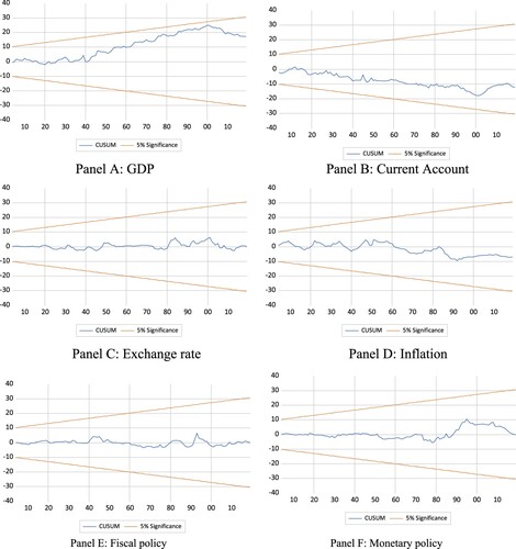
We address the potential issue of a structural break in three different ways. First, we include one dummy variable for each of the policy regimes in the main model estimation as exogenous variables. These dummy variables control for changes in the mean, such as a lower trend growth rate or equilibrium interest rate across the policy regime. Second, we test if there is a structural break in the parameter vector using a CUSUM-test (Brown, Durbin, & Evans, 1975). Third, we split the sample into shorter sub-samples and re-estimate the model for each sub-period. Unfortunately, several of the policy regimes are too short (fewer than twenty observations) for us to estimate the model for each regime separately. Instead, we rely on longer sub-sample periods.

We consider two ways of splitting the sample. In the first case, we split the full sample into two halves: one half representing 1873–1951 and the other half representing 1952–2019. The first period represents a period of relatively modest stabilisation polices, and the second period represents the time when active stabilisation policies became the norm. In the second case, we split the sample into three sub-samples. The first sub-sample combines the gold standard and the off–on gold period into one, representing a time when monetary policy mostly followed the rules of the gold standard and fiscal policy aimed at a balanced budget. The second sub-sample represents the experiment and Bretton Woods periods, when fiscal and monetary policy were coordinated, and foreign capital flows were restricted. The third sub-sample combines full employment and norm policies: two regimes when the exchange rate in practice was adjustable, and there were no or limited restrictions on international capital flows.

The CUSUM test show that we cannot reject the null hypothesis of no structural break (see Appendix C), i.e. that the parameter vector is stable over the sample period. Furthermore, partitioning the sample has only minor effects on the results (see the robustness analysis in the section Robustness of the Results). In those cases, there is a significant difference in the results: the shock estimates from the full sample are more in line with the history outlined in the descriptive literature. We thus use the full sample estimations as our benchmark results, while also illustrating the shocks from the sub-sample period in the robustness section.

3.2. Data and descriptive statistics

Detailed information about the data sources are available in Appendix A. The variables are illustrated in Figure 1, and Table 2 presents descriptive statistics, including the average and the standard deviation. We use yearly data as quarterly and monthly data for GDP⁹, the current account and the public debt is not available.

Figure 1. Economic and policy variables 1873–2019.

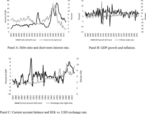
Table 2. Summary statistics.

	Debt ratio	Interest rate	GDP growth	Inflation	Current account	Exchange rate
Full sample 1873–2019	27.1 (16.0)	4.9 (2.7)	2.7 (3.0)	3.0 (2.2)	0.1 (3.3)	5.18 (1.70)
Gold standard 1873–1914	16.0 (2.6)	4.8 (0.7)	2.4 (2.2)	0.4 (3.4)	−2.5 (2.1)	3.70 (0.13)
Off-on gold 1915–1931	17.6 (2.1)	5.2 (1.0)	2.4 (5.0)	3.7 (15.5)	1.6 (4.2)	3.80 (0.41)
Experiment 1932–1951	29.5 (10.2)	2.8 (0.5)	3.5 (4.6)	3.5 (5.3)	0.6 (2.4)	4.23 (0.49)
Bretton Woods 1952–1973	16.7 (4.0)	4.7 (1.1)	3.8 (1.6)	4.1 (2.1)	0.0 (0.9)	5.12 (0.18)
Full employment 1974–1992	42.7 (14.9)	10.0 (2.6)	1.7 (1.7)	8.4 (2.9)	−1.6 (1.3)	5.80 (1.37)
Norm policies 1993–2019	46.6 (16.3)	2.7 (2.6)	2.5 (2.2)	1.4 (1.2)	4.1 (2.5)	7.75 (1.01)

Note: The top figures illustrate the average values during the period. The values in parentheses are the standard deviations.

The public debt ratio was more or less stable from the gold standard through Bretton Woods. It then increased during full employment to a higher level, which was maintained, on average, during norms. However, as revealed by Figure 1, debt rose almost linearly during full employment and fell almost linearly during norms. The volatility in public debt and the short-term interest rate increased over time, while the volatility in the GDP growth rate and the inflation rate declined. The current account balance and the exchange rate were stable during Bretton Woods when maintaining external balance was a key policy priority. The exchange rate was more volatile during full employment when devaluations were frequent compared with norms when the exchange rate floated freely on the exchange rate market.

Inflation was low during the gold standard, but the volatility was relatively high. The most stable inflation rate was during norms. GDP growth increased on average until full employment. It declined thereafter. In terms of overall economic stability, no regime stands out as the most successful in terms of providing stability for the entire economy.

4. Swedish Fiscal and monetary policy shocks

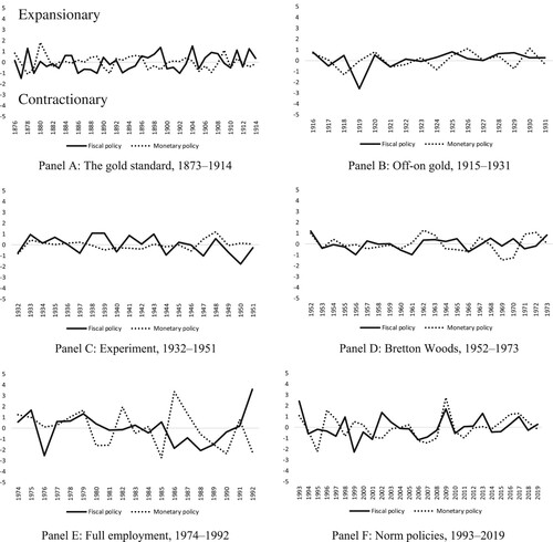
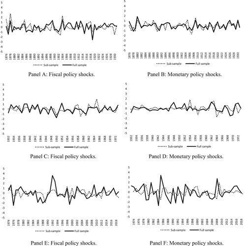
Figure 2 illustrates the estimated fiscal and monetary policy shocks. Figure 2 consists of six panels, one for each policy regime. A positive fiscal policy shock – in other words, a higher public debt – implies an expansionary policy change. A positive monetary policy shock – that is, a higher interest rate – implies monetary tightening. To make the interpretation of the results easier, we transformed the monetary shock so that a negative shock implies a monetary tightening similar to the fiscal shocks.¹⁰

Figure 2. Fiscal and monetary policy shocks, 1873–2019.

The standard deviations of the policy shocks are shown in Table 3. The variance is normalised to one for the full sample period. A standard deviation greater (lower) than one during a specific regime thus indicates a more (less) volatile regime compared with the full sample average. Table 3 presents both the estimated variance of the policy shocks and the estimated shocks coming from the other variables in the model.

Table 3. Estimated standard deviations of the fiscal and monetary policy shocks.

	Policy			Economy
	Fiscal policy	Monetary policy	GDP growth	Current account	Exchange rate	Inflation
Gold	0.77	0.60	0.76	0.94	0.36	0.90
Off-on-off	0.86	0.72	1.36	0.80	1.13	1.40
Experiment	0.83	0.44	1.36	1.42	1.09	1.06
Bretton Woods	0.56	0.73	0.57	0.48	0.33	0.66
Employment	1.43	1.66	0.83	0.91	1.33	0.86
Norm	0.98	1.06	0.62	0.74	1.14	0.62

Note: The variance is normalised to 1 over the entire sample period.

Policy shocks prior to full employment (1974–1992) are relatively small, with an estimated standard deviation of less than one. The smallest policy shocks are for Bretton Woods, which may seem strange considering that this was considered to be the heyday of traditional Keynesian policies. However, policymakers relied on a larger toolbox during that era. Partially because credit and foreign exchange controls enhanced their control over the economy, and partially because self-imposed restrictions on domestic and international borrowing as well as a fixed exchange rate, which in effect limited their ability to use the budget balance and the interest rate to stabilise the economy (Lindbeck, 1973, 1997).

An illustration of the relatively small size of the shocks is the so-called ‘Fool’s Stop’ policy (‘Idiotstoppet’) in 1969/70. Monetary policy was tightened at the time against the critiques from both the political opposition and many economists. The sizes of the monetary policy shocks were −1.5 in 1969 and −1.3 in 1970. At the time, these shocks were large; the standard deviation during Bretton Woods was 0.73. However, they were average in size compared to the shocks during full employment (1.66) and norms (1.06).

The policy shocks during the gold standard show patterns of frequent policy reversals: an expansionary policy one year is followed by a contractionary policy the next (see Panel A). Economic policies became more persistent over time, with expansions and contractions often lasting a few years at a time.¹¹ Both poorer economic planning and a lack of data on the state of the economy potentially explain the policy reversals during the gold standard. For example, a fiscal budget overestimates revenue one year or miscalculates the cost of a government programme, creating a deficit that due to the implicit balanced budget rule requires a fiscal tightening the following year. Similarly, an increase in the Riksbank’s reserves one year may cause a relatively large interest rate cut, which causes a drain on the reserves and the need for a policy reversal.

The macroeconomic volatility has varied over time. The most volatile period is off–on-gold, which includes the First World War, the 1920s disinflation, and the first stages of the Great Depression. The subsequent experiment is also volatile, as it includes the Great Depression and the Second World War. The volatility in the economic variables is relatively similar for the other policy regimes. For example, the volatility in GDP growth and the current account was 0.76 and 0.94 during the gold standard, respectively, compared with 0.62 and 0.74 during the norms. These results suggest that differences in how stable the economy is over time depend less on changes in the macroeconomy and more on changes in economic stabilisation policies. Stabilisation policies are both a source of enhanced stability and destabilisation.

4.1. Fiscal and monetary policies during elections

Fiscal, but not monetary, policy largely follows a political cycle. Figure 3 illustrates the combined policy shock for fiscal policy (Panel A) and monetary policy (Panel B) during a general election year and the year prior to the election. Here, we focus on the period from the 1930s onwards, after full male and female suffrage was established. A black bar in Figure 3 indicates a government that was returned after the election, and a grey bar indicates a change of government.

Figure 3. Fiscal and monetary policy shocks during general elections, 1932–2018. Notes: a. The figures illustrate the combined effect during the election year and the year prior to the election year; b. elections that resulted in a change in government are illustrated with grey bars.

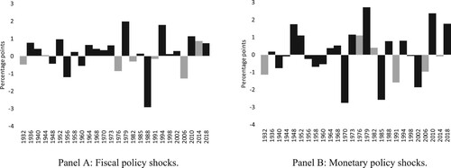
Fiscal policy was expansive during 16 of the 26 general elections. Five out of the ten times that fiscal policy was contractionary, it resulted in the election of a new government (1932, 1976, 1982, 1991, 2006). On three occasions, the government (including its parliamentary support) suffered losses when fiscal policy was contractionary but held on to power (1948, 1956, and 1988). The only election when fiscal policy was contractionary and the government performed well was in 1960. The only time fiscal policy was expansionary and the government lost the election was in 2014. In other words, there are clear signs of political cycles in terms of fiscal policy. The introduction of norm policies in the 1990s may have reduced the overall government debt level, but it has not restrained governments from stimulating the economy prior to elections. The shift from a four-year to a three-year parliament between 1970 and 1994 made the policy interventions more frequent and added to the volatility of the economy. Similarly, the shift back to a four-year parliament after the 1994 election likely contributed to greater economic stability.

We find no clear relationship between elections and monetary policies. There are 12 elections with contractionary policies and 14 elections with expansionary policies. The fixed exchange rate prior to 1992 and an independent Riksbank after 1993 limited the use of monetary policies during election times. However, monetary policy was expansionary in four out of six elections during full employment, when the exchange rate was fixed but regularly adjusted.

4.2. Policies during major economic crises

Sweden suffered from nine major crises during the sample period (Fregert & Jonung, 2018; Jonung, 2019): five financial crises (1878/79, 1907/08, 1929–33, 1991–93, and 2008/09); indirectly two wars (First World War, 1915–1918 and Second World War, 1940–1945); and two other episodes (deflation policy during 1921/22 and the 1973–1979 OPEC oil crises). Table 4 outlines the economic policies during the crises and the immediate years following the respective crises. ‘Immediate years’ are defined as the years following the crisis until there was a change in policy indicated by a shift from expansionary to contractionary policies, or vice versa.

Table 4. Fiscal and monetary policy shocks during major economic crises.

Episode	Fiscal policy	Monetary policy
Financial crisis 1878/79	1878: +1.3 1879: −1.0	1878/79: −1.6 1880/81: +2.5
Financial crisis 1907/08	1907/08: +1.7 1909/10: −0.6	1907/08: −1.2 1909: +1.1
World War I 1915–1918	1915: −1.3 1916: +0.8 1917: −0.5 1918: +0.5	1915: −0.8 1916/17: +0.7 1918: −1.3
Deflation policy 1921/22	1919: −2.6 1920: +0.5 1921: −0.6	1921-24: −1.6
Financial crisis 1929–1933	1929/30: +1.0 1931/32: −0.7 1933-36: +1.9	1930: +1.2 1931/32: −1.2 1933-37: +1.0
World War II 1940–1945	1940: −0.7 1941-43: +2.0 1944-47: −1.7	1940-46: −1.6 1947/48: +1.7
OPEC I and II 1973–1979	1973-75: +3.0 1976: −2.5 1977-80: +3.0	1973-79: +6.5 1981/82: −3.1
Financial crisis 1991–1993	1991-93: +6.2 1994-97: −2.0	1991: +0.8 1992: −2.2 1993: +1.1 1994/95: −2.5
Financial crisis 2008/09	2008: −0.3 2009: +1.7 2010: −0.6	2008: −1.0 2009: +2.8 2010-12: −1.4

4.2.1. Policies during financial crises

Four of the five financial crises were international crises spilling over into Sweden, and one crisis was a largely domestic crisis (the 1991–1993 banking crisis). Monetary policy was contractionary during the 1878/79 and the 1907/08 crises due to a drain on the gold reserves. The policy was then fully reversed once the crisis was over. Fiscal policy, in contrast, was expansionary during both crises: in the 1878/79 crisis, during the first crisis year before the policy was neutralised in 1879; and during the entire 1907/08 crisis. In the latter crisis, fiscal policy was neutralised in 1909/10. In other words, discretionary fiscal policy provided support for the real economy for at least part of the financial crisis. As discussed in Section 2, most of the support was through financial support to the banking sector rather than aimed at stimulating the real economy. Fiscal policy continued to provide support for the economy during the early crisis phase throughout all financial crises. Monetary policy was expansionary during the early stages of all financial crises from the Great Depression onwards. Fiscal and monetary policies provided support for the economy during 1929/30, prior to the election of the Social Democratic government in September 1932, which is often credited with introducing Keynesian stabilisation policies in Sweden. A run on the Riksbank’s gold reserves in 1931 following the collapse of the Creditanstalt in Austria forced a policy shift to contractionary policies to defend the exchange rate.

The same behaviour is observed during the crisis of the 1990s. Fiscal and monetary policies became expansionary during the early stages of the crisis in 1991. The European exchange rate crisis in 1992 caused a policy shift to contractionary monetary policies until the fixed exchange rate was abandoned in November 1992. The fixed exchange rate, both in the 1930s and the 1990s, was an obstacle preventing the policymakers from continuing their policies in the real economy in favour of a contractionary policy defending the fixed exchange rate. Policymakers had to choose between international economic balance and stable exchange rate.

In the 1930s, the suspension of the gold standard led to expansionary fiscal and monetary policies. The yearly expansionary shocks were small, but they lasted for several years; fiscal policy was expansionary from 1933 to 1936, and monetary policy was expansionary from 1933 to 1937. The combined effect during these years were thus sizeable. In the 1990s, policy reverted to being expansionary after the ERM crisis, when the fixed exchange rate was abolished, which is similar to the 1930s crisis. However, both fiscal and monetary policies then became contractionary again during the economic recovery phase. Here, the economic recovery was clearly dampened by the policy failures during full employment. A large and unsustainable public debt ratio forced fiscal consolidation during the recovery. A poor inflation record, for almost twenty years, forced the Riksbank to set high interest rates and depress economic activity to build public confidence for its commitment to the newly adopted inflation target. It was easier for policymakers to sustain a long period of expansionary policies in the 1930s because the public debt ratio was low and the recent memory was of deflation rather than high inflation. One of the reasons a price level target was introduced in 1932 was the memory of the deflation crisis of the 1920s. On both occasions, the policy responses to the crisis and the recovery were partially shaped by the memory and policy actions of the preceding years.

The international financial crisis of 2008/09 was the only financial crisis Sweden faced with a flexible exchange rate, which makes it an interesting case to compare with the other crises with a fixed exchange rate. However, the international financial crisis had no major impact on the Swedish banking system and housing market, and hence it is difficult to draw any definite conclusions. Nevertheless, there are indications of the flexible exchange rate assisting the policymakers in stabilising the real economy. First, the exchange rate depreciated by 15–20 percent against the euro, reducing the need for a fiscal or monetary stimulus. Second, monetary policy was expansionary in 2009, with a policy shock of +2.8. This was reversed as the economy began to recover in 2010.

In sum, we find that fiscal policy was expansionary during each financial crisis, although it sometimes had to become contractionary to help defend the fixed exchange rate. To defend the exchange rate, the Riksbank had to pursue a contractionary policy during at least parts of the crises, thus worsening the real economic effects of the crises. Although a fixed exchange rate may provide stability during normal times, in times of crises, it forced the Riksbank to put the defence of the exchange rate ahead of the real economy. The economy suffered as a result in the middle of the crises, deepening and prolonging the crises.

4.2.2. Policies during the World Wars

Economic policies during the First World War followed in the footsteps of the policies during the gold standard. Both fiscal (−1.3) and monetary (−0.8) policies were contractionary in 1915, despite Sweden abandoning the gold standard in August 1914, which opened up the opportunity for a more expansionary policy. The fiscal contraction was fully reversed in 1916, although it took two years to reverse the monetary contraction. We find that both fiscal and monetary policies were on average neutral between 1915 and 1917. They then become contractionary in 1917/18, just as the Swedish economy began to suffer from weaker export demand. The shift in policy was possibly due to the increase in inflation which hit a record of 47 percent in 1918 due to the combined effect of war shortages and a previously booming economy. Overall, policy provided little support to stabilising the economy during the war, similar to much of the preceding gold standard period.

The policy response during the Second World War was clearly different. Fiscal policy was expansionary, with a combined shock effect of +2.0 between 1941 and 1943. The majority of the increase in expenditures was for military purposes. The fiscal expansion was accompanied by a mild monetary contraction of −1.6 between 1940 and 1946. Fiscal and monetary policies were coordinated during this period, and the monetary contraction allowed for a fiscal expansion while keeping inflationary pressures under control. The public finances were consolidated between 1944 and 1947 (−1.7), after the risk of a German invasion subsided during 1943/44. The coordination with monetary policy is again visible, as there was a monetary loosening in 1947/48 (+1.7), allowing for an expansion of private activity once the inflation risk had subsided. The coordination of fiscal and monetary policies during this period contributed to more stable economic development compared with the First World War years.

4.2.3. Policies during deflation crisis and OPEC I and II

Sweden experienced two crises that were unrelated to wars and financial crises: the deflation crisis of 1921/22 and the OPEC I and II oil price crises of 1973–1979. Prices fell rapidly during the deflation crisis, totalling a decline of 36 percent between 1921 and 1922. However, the price level remained 70 percent higher compared with prior to the First World War. Nevertheless, the gold standard was de facto reinstated in November 1922 and de jure reinstated in April 1924. According to our estimates, monetary policy was contractionary throughout the disinflation period, but the contraction was relatively small (in total −1.6 percentage points between 1921 and 1924). Fiscal policy was also contractionary (−2.6) in 1919, only slightly relaxed in 1920, and then made even more contractionary in 1921 (−0.6). Although the fiscal contraction was relatively large, even by modern standards, the total effect was unlikely to be sufficient to generate such a large deflation. According to our estimates, most of the disinflation came from a weak international economy after the war, rather than from domestic disinflation policies. This result may explain why policymakers at the time were surprised by the rapid decline in prices (Lundberg, 1985). They simply misjudged the international business cycle and pushed through contractionary policies when the Swedish economy was severely weakened by declining international demand.

The second major crises are the OPEC I and II crises. OPEC I caused the first major post-Second World War recession and led to rising inflation (so-called ‘stagflation’). In line with classic Keynesian thinking, the policy response was to ‘bridge over’ the recession by making fiscal policy and monetary policy highly expansionary to simulate the economy and thus avoid the recession. The expectation was that the international economy would soon revert to pre-OPEC growth. The combined fiscal shock was +3.0 percent between 1973 and 1975. The borrowing was so heavy that the government borrowed internationally for the first time since prior to the Second World War. Growing debt led to a contraction in 1976 of −2.5 percentage points, but the policy was fully reversed over the four-year period from 1977 to 1980. Monetary policy became expansionary in 1973 and remained so until 1979, with a combined shock of +6.5 percentage points. There is no other period in Swedish economic history with more persistent and large expansionary policy shocks. It was partially caused by a misreading of the OPEC crisis, expecting it to be temporary and for global growth to quickly pick up (Lundberg, 1983). When this failed to materialise, the policy response was to continue with more doses of economic stimulus.

Both the deflation crisis of the 1920s and the OPEC crises of the 1970s caused severe economic difficulties which, after a decade, resulted in two new stabilisation policy regimes (experiment and norm, respectively) aimed at avoiding repeating the mistakes of these two crises. The policy mistakes were on both occasions caused by a misreading of the international economy and applying the policy rules of the past in a new economic climate.

4.3. Summary

Our results both confirm previous results from the qualitative literature and provide new insights. Similar to previous studies, we find that the sizes of discretionary fiscal and monetary policies were relatively small until the 1930s and that the size of the shocks grew substantially after the 1970s. Institutional arrangements matter. The gold standard and the fixed exchange rate clearly acted as obstacles to policymakers supporting growth during crises, and they had to shift to defending the exchange rate rather than the real economy in the middle of the crises. Economic stability during the Bretton Woods years collapsed because of the oil price shocks and increased political competition, which reduced the self-imposed discipline to maintain a balanced budget and a balanced current account.

In contrast to previous studies, we find that policymakers quickly learned how to respond to financial crises to limit their effects on the real economy. Discretionary fiscal policy was expansionary during the 1878/79, 1907/08, and 1929/30 crises. Previous studies have highlighted the 1930s as the starting point of Keynesian stabilisation polices during crises, yet our results reveal that such behaviour in fact existed much earlier, either by good luck or a deliberate policy. The deflation crisis of the 1920s was mostly the outcome of external events and not Swedish fiscal and monetary policies. Yet the domestic policy memory of the crisis was important for how policymakers responded to the crisis of the 1930s. The fiscal and monetary policy shocks during the Great Depression were relatively small on a yearly basis. However, policies remained expansionary over several years, and therefore the cumulative effect was sizeable.

The budget balance and the short-term interest rate played minor roles in the stabilisation policy regimes during Bretton Woods until the so-called ‘Fool’s Stop’ in 1969/70. Yet the fiscal shocks in those two years were moderate compared to the size of the shocks in the later full employment and norms regimes. Although the government actively intervened in the economy, it did so by using a larger toolbox than the interest rate and the fiscal balance. It was first following OPEC I that the interest rate and the fiscal balance began to play key roles as stabilisation tools. The introduction of an inflation target and strict fiscal rules did not prevent an active stabilisation policy. The sizes of the shocks were not much smaller than during full employment. However, the average inflation rate was lower, and the government debt declined from 75 percent in 1995 to35 percent in 2019. The norms period thus provided for greater long-term stability but did not limit the policymaker from actively using fiscal and monetary policies in the short run. In other words, the inflation target and the fiscal rules are primarily long-run anchors for economic policies similar to the gold standard.

Finally, perhaps the most important result from our analysis is the finding that the evolutions of several stabilisation policy regimes follow a similar pattern. All new regimes came about as a response to the failures of the previous regime. Most regimes work well for a few years before new economic and political circumstances result in a string of policy mistakes – in our data, represented by either higher volatility in the shocks or longer periods of expansionary or contractionary policies. It appears that the policymakers struggled to achieve their objectives, and rather than rethinking policy, they continued with the same policy with greater vigour. In our sample, this is represented by an increase in the size of the policy shocks. The high volatility increased volatility in the economy, contributing to ending the regime and introducing a new regime a few years later.

5. Robustness of the results

We test the robustness of the results by considering the possibility of a structural break in the parameters. To this end, we split the sample period into sub-samples. Unfortunately, we cannot estimate the model policy regime by policy regime, as some of the regimes are too short. For example, the off–on gold regime lasted only 16 years, which is too short to provide trustworthy estimates. Instead, we split the sample into longer periods by combining several policy regimes.

The sample is split in two different ways. First, we split the sample into two almost equal halves representing 1873–1951 (gold standard, off–on gold, and experiment) and 1952–2019 (Bretton Woods, full employment, and norm). Second, we decompose the sample into three periods. First, we combine the gold standard and off–on gold, since they are relatively similar in terms of institutional arrangements. Second, we combine experiment with Bretton Woods. These regimes are similar in terms of policy aims, coordination of fiscal and monetary policies, and (for most of the period) credit and foreign exchange controls. Finally, we combine full employment and norm. Financial liberalisation began under full employment and the policy of a flexible exchange rate was introduced in practice during this regime.

Table 5 contains the correlations between the shocks from the full sample and the respective sub-samples. The correlation is consistently high, always above 0.5, and often in the range of 0.6 and 0.8. The correlation is lower for the shorter sub-samples compared with the longer sub-samples. The parameter estimates, and thus the policy shocks, are automatically more uncertain when they are estimated using fewer observations. The lower correlation with the full sample shocks is thus likely caused by a larger estimation error in the sub-sample estimations compared with the full sample. The shorter sample period also makes the estimation more sensitive to data outliers caused by, for example, an economic crisis.

Table 5. Correlation between policy shocks from sub-samples and the full sample.

Sub-period estimation	Fiscal policy	Monetary policy
Gold, off-on gold, and Experiment 1873–1951	0.74	0.71
Bretton Woods, full employment, and norm policies 1952–2019	0.74	0.80
Gold and off-on gold 1873–1931	0.54	0.56
Experiment and Bretton Woods 1932–1973	0.60	0.53
Full employment and norm policies 1974–2019	0.58	0.73

Figure 4 compares the shocks from the three sub-samples with the shocks from the full sample. The figure confirms the results from the correlations in Table 5. The movements during the respective policy shocks are similar. The greatest difference between the shock estimates is for the smaller shocks which, from an economic point of view, are the less interesting shocks. One exception is during the financial crisis of the early 1990s, when the volatility of the monetary shocks is higher for the full sample estimation compared with the sub-sample estimation. In 1990, 1991, and 1993, the interest rate varied by 3–4 percentage points on a yearly basis within the range of 10–14 percent. In 1992, it increased from 11.5 percent in June to a high of 500 percent in September during the defence of the fixed exchange rate, before it fell back to 11.5 percent in December after the Riksbank abandoned the krona peg to the European Currency Unit (the ECU). Given the volatility of the interest rate, the full sample shocks appear to give a more accurate account of the volatility in the policy than the sub-sample shocks.

Figure 4. Comparison of the policy shocks from the full sample with shocks from the subsamples.

Another period of relatively large differences in the estimated shocks occurs towards the end of the sample period when the Riksbank experimented with a negative interest rate and quantitative easing (Andersson & Jonung, 2020). According to the full sample period, monetary policy is expansionary when interest rates are negative. According to the sub-sample estimation, monetary policy is neutral or even contractionary policy at this time. It is unlikely that a negative interest rate indicates a neutral or contractionary policy when inflation was close to the inflation target, the employment rate was the highest it had been for 30 years and GDP growth was in the range of 2–4 percent for more than five years. Consequently, we conclude that the full sample policy shocks provide the most accurate account of economic policy. However, it should be noted that in most cases, the differences in the estimations are small, indicating that the results are robust.

6. Conclusions

Our analysis of Swedish stabilisation policies in the period 1873–2019 provides four key results. First, we find that discretionary policies are often a great source of economic instability. Economic volatility in the macroeconomic variables is relatively constant throughout time, apart from during the First and Second World Wars. The volatility in the policy shocks, however, varies over time, indicating that stabilisation policies are partially a source of instability rather than stability. Over time, the variation in the policy shocks is more than the shocks of the macroeconomic variables such as inflation and GDP growth.

During the gold standard, the policy shocks were small, and policies swung from contractionary to expansionary – and vice versa – on a yearly basis. Policy reversals became less frequent, yet the sizes of the policy shocks were similar from the 1930s throughout the 1960s. This is considered one of the more stable periods in Sweden’s economic history. The size and the duration of the policy shocks increased substantially in the 1970s and 1980s. The introduction of an inflation target or fiscal policy rules did not limit the short-run volatility of the shocks. However, they did provide a long-run policy anchor.

The second result is that all policy regimes fail as the economic circumstances change. An early indication of the collapse of a regime is increased volatility of the policy shocks. As the stabilisation policy no longer provides a similar result as in the past, the policymaker responds initially by increasing the size of the shocks rather than updating the policy. The increased size of the shocks creates economic instability and, eventually, policy rethinking and a new policy regime.

The third result is that institutional arrangement matters. Strict rules, such as those provided by the gold standard, fixed exchange rate or inflation target, provide policy certainty. They can also become destabilising, as illustrated in times of financial crises from the 1870s until the 1990s, when the gold parity or fixed exchange rate forced policymakers away from supporting the real economy to supporting the exchange rate, thus worsening the recession. There is no evidence of explicit rules being more successful than implicit, self-imposed rules. The Bretton Woods period provided a stable economy and stable public finances through self-imposed balanced budget and balanced current account rules. Explicit rules may become destabilising by preventing policymakers from responding to new circumstances. However, no rules may also cause instability, as demonstrated by the full employment regime. The fourth and final result is that the present policy regime is unlikely to be the last. The quest for a long-lasting stabilisation policy will continue in the future.

Disclosure statement

No potential conflict of interest was reported by the author(s).

Notes

1 Papers exploring part of the post-WWII period include the work of Cloyne and Hürtgen (2016), Kuttner (2001), Romer and Romer (1989) and Romer and Romer (2004).

2 Papers studying the pre-WWII period include the work of Bordo and MacDonald (2003), Jeanne (1995), Lennard (2019) and Parker and Rothman (2004).

3 Foreign exchange controls were partially relaxed in 1958 when the Swedish krona was made convertible for ongoing transactions, but not for investments (Werin et al., 1993; Wetterberg, 2009).

4 The Social Democratic party formed the government between 1932 and 1976, with the exception of June to September 1936. They were in coalition with the Farmer’s League (later, the Center Party) from 1936 to 1939 and 1951–1957. There was a grand coalition among all parties except for the Communist Party during WWII. Regular changes of government have taken place since 1976.

5 The currency basket was replaced by a peg against the European Currency Unit in 1991.

6 Romer and Romer (2004) introduces a narrative approach where they estimate a regression model based on data included in the Federal Reserve’s Greenbook. This reduces the subjectivity of the method and is closely related to the SVAR model approach.

7 An alternative variable is the unemployment rate but historical estimates of unemployment before the early 1900s are scares.

8 We use the Bayesian (Schwarz) information criterion. It indicates including two lags in the model. Adding a third lag to the model has no significant impact on our results.

9 Edvinsson and Hegelund (2018) provides estimates of quarterly GDP stretching back to 1913.

10 The monetary shocks are given by e_i in equation (1(1) $A_0{y}_t=c+\sum _{i=1}^I{A}_i{y}_{t-i}+\sum _{j=o}^J{D}_j{x}_{t-j}+e_t$(1) ). We are illustrating -e_i so that a higher shock implies a monetary expansion to make the monetary shocks comparable to the fiscal shocks.

11 The autocorrelation of the fiscal policy shocks increases slowly over the regimes from -0.2 during the gold standard to +0.2 during full employment. It then declines to -0.1 during norm policies when the surplus target is introduced. For monetary policy shocks the increases from -0.1 during the gold standard to +0.3 during full employment. The autocorrelation declines to -0.1 during norm policies.

Appendices

Appendix A. Data sources

Table A1. Data sources.

Variable	Data source
GDP	1873–1950 Schön and Krantz (2015), 1951–2019 Statistics Sweden.
Current account balance in relation to GDP	1873–2016 Jordá, Schularick, and Taylor (2017), 2017–2019 Statistics Sweden.
Exchange rate SEK vs. USD	1873–1914 Lobell (2010), 1915–2008 Bohlin (2010), 2009–2019 Swedish Riksbank.
Inflation	1873–2019 Statistics Sweden.
Short term interest rate (monetary policy)	1873–2012 Waldenström (2014), 2013–2019 Swedish Riksbank.
National debt (fiscal policy)	1873–2011 Fregert and Gustafsson (2014), 2012–2019 Swedish debt office.
US and UK GDP	Bolt and van Zande (2020)
US inflation	Officer and Williamson (2021).
UK inflation	Clark (2021).
Oil prices	U.S. Energy Information Administration

Electronic Data Sources

Angus Maddison Statistics

http://www.ggdc.net/maddison/oriindex.htm

Measuring worth

https://www.measuringworth.com/

National debt office statistics

https://www.riksgalden.se/en/statistics/

Swedish Riksbank Statistics.

https://www.riksbank.se/en-gb/statistics/

Statistics Sweden.

https://scb.se/en/

St. Louis Fred Database

https://fred.stlouisfed.org/series/GDPC1

U.S. Energy Information Administration

https://www.eia.gov/dnav/pet/hist/LeafHandler.ashx?n=PET&s=F000000__3&f=A

Appendix B: Estimation results and impulse response functions

The fiscal and monetary policy shocks are identified using the SVAR model in Equation (1). However, it is not possible to estimate this model directly due to the contemporaneous effects. Instead, we first estimate a reduced form VAR model (Equation 2), and then apply a Cholesky decomposition to identify the policy shocks in Equation (1) using the estimation results from the VAR model. The parameter estimates from the VAR model are shown in Table B.1.

Table B1. VAR model estimation results.

	GDP	Current Account	Exchange rate	Inflation	Fiscal Policy	Monetary policy
GDPt-1	.05 (.11)	-.12* (.07)	.10 (.40)	-.27** (.13)	-.21** (.09)	.02 (.03)
GDPt-2	-.09 (.10)	.01 (.07)	-.02 (.39)	.19 (.12)	-.04 (.09)	-.00 (.04)
CAt-1	.15 (.13)	.73*** (.10)	−1.46*** (.52)	.11 (.17)	-.17 (.13)	.03 (.05)
CAt-2	-.14 (.15)	-.00 (.10)	.87 (.56)	.47 (.18)	-.12 (.14)	-.06 (.05)
Exchange ratet-1	-.01 (.02)	-.00 (.02)	.08 (.09)	.03 (.03)	-.02 (.03)	.01 (.01)
Exchange ratet-2	-.00 (.02)	.04** (.02)	-.29*** (.09)	.06** (.03)	-.04* (.02)	.01 (.01)
Inflationt-1	.01 (.08)	-.20*** (.05)	.43 (.30)	.20** (.10)	-.04 (.07)	.03 (.03)
Inflationt-2	.11* (.07)	.00 (.05)	-.42 (.28)	-.26*** (.09)	04 (.07)	.00 (0.03)
Fiscalt-1	-.03 (.10)	-.11 (.07)	-.14 (.40)	-.01 (.13)	.63*** (.10)	-.10*** (.04)
Fiscalt-2	.18** (.09)	.05 (.07)	.43 (.37)	-.04 (.11)	-.13 (.09)	.09*** (.03)
Monetaryt-1	-.43** (.21)	.05 (.17)	.63 (.91)	.49* (.30)	.56*** (.22)	.67*** (.08)
Monetaryt-2	.10 (.23)	.03 (.16)	−1.02 (.89)	-.48* (.29)	-.48** (.21)	.12 (.08)
GDP USAt	-.05 (.05)	.01 (.04)	-.01 (.02)	-.01 (.01)	.02 (.045)	.02 (.02)
GDP USAt-1	.05 (0.05)	.07* (.03)	-.02 (.02)	-.01* (.01)	.07* (.05)	.01 (.02)
GDP USAt-2	-.07 (0.09)	-.03 (.03)	-.15 (.18)	.06 (.06)	.05 (.05)	.02 (.02)
GDP UKt	-.08 (.09)	.04 (.06)	-.03 (.35)	.40*** (.11)	.05 (.08)	-.01 (.03)
GDP UKt-1	.24*** (.10)	.05 (.06)	.14 (.40)	.13 (.13)	-.15 (.10)	.00 (.04)
GDP UKt-2	.11 (.09)	.05 (.06)	.30 (.35)	.07 (.11)	-.04 (.09)	.01 (.03)
Inflation USAt	.46*** (.10)	-.13* (.07)	.05 (.38)	.21* (.12)	-.40*** (.09)	-.00 (.04)
Inflation USAt-1	-.21** (.10)	-.03 (.08)	-.25 (.44)	.34*** (.14)	.31*** (.11)	-.00 (.06)
Inflation USAt-2	.41*** (.10)	.03 (.07)	.33 (.32)	−43*** (.12)	-.35*** (.09)	-.00 (.04)
Inflation UKt	-.25*** (.08)	.10** (.05)	-.20 (.30)	.53*** (.09)	.13* (.07)	.02 (.03)
Inflation UKt-1	-.16 (.10)	.20*** (.07)	-.55 (.36)	-.07 (.12)	-.05 (.09)	-.04 (.03)
Inflation UKt-2	.32*** (.09)	-.03 (.07)	.63* (.36)	-.07 (.12)	-.05 (.09)	-.04 (.03)
Oilt	.01 (.01)	-.00 (0.01)	.02 (.04)	-.01 (.01)	.00 (.01)	.01*** (.00)
Oilt-1	-.01 (.01)	.00 (.01)	-.01 (.04)	-.01 (.01)	.02* (.09)	.00 (.00)
Oilt-2	-.02** (.01)	.00 (.01)	.04 (.04)	-.01 (.01)	.00 (.01)	.01 (.00)
Gold	.18 (.93)	−1.32** (.64)	−1.60 (3.52)	1.37 (1.14)	−1.80** (.85)	-.18 (.33)
Return	-.71 (.90)	.25 (.62)	1.10 (83.40)	-.51 (1.10)	.47 (.82)	.79*** (.32)
Experiment	−1.58* (.83)	.42 (.57)	2.72 (3.13)	1.49 (1.01)	.47 (.82)	.79*** (.32)
Bretton	-.64 (1.06)	2.10*** (.76)	−1.84 (4.19)	3.88*** (1.36)	.09 (1.01)	−1.41*** (.39)
Employment	3.33*** (1.27)	−3.73*** (.88)	−3.22 (4.80)	−2.37 (1.56)	-.92 (1.16)	−1.41*** (.39)
Constant	3.56*** (1.03)	.24 (.71)	3.92 (3.89)	−5.84*** (1.27)	1.04 (.94)	.02 (.36)
Adj R^2	.53	.82	.34	.83	,68	.93

Note: *, **, and *** denote statistical significance at the 10%, 5% and 1% significance level respectively.

Having identified the structural shocks in Equation (1), we can then estimate the effect on one variable on another variable in the model. As an illustrated we illustrate the effect of a contractionary fiscal policy shock on the economy in Figure B.1 and the effect of a contractionary monetary policy shock on the economy in Figure B.2.

Figure B1. Estimated economic effects of a contractionary fiscal policy shock.

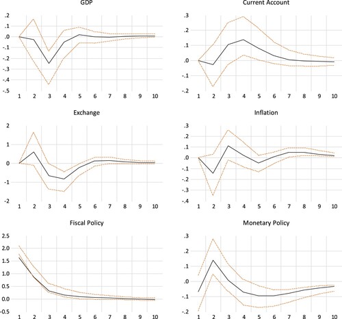
Figure B2. Estimated economic effects of a contractionary monetary policy shocks.

The estimated effects of a contractionary fiscal and monetary policy shock are in line with theory. GDP growth declines with the maximum effect reached after two to three years. The current account improves and there is an appreciation of the exchange rate. Inflation falls after a contractionary monetary policy shock after three years. The effect of a fiscal policy shock on inflation is somewhat weaker. A contractionary fiscal policy shocks is initially followed by a tightening of monetary policy which is then reversed and becomes expansionary as growth declines and the current account improves.

That the economic response of the estimated policy shocks on the economy is in line with theory is an indication that the estimated shocks are reasonable estimates of the true policy shocks.

Appendix C: CUSUM stability test

We test for a structural break in the parameter vector using a CUSUM test (see e.g. Brown et al., 1975). The test provides a test-statistic for each year of the sample period and an upper and lower bound. The null hypothesis is that there is no structural break in the parameter vectors, i.e. the parameters are stable throughout the sample period. The test indicates a structural break if the test-statistic moves outside the critical bounds. Figure C1 illustrates the test for each endogenous variable in the regression.

The test-statistic stays within the boundaries for each variable throughout the sample period. The only variable the test comes close to the boundaries is for GDP in the year 2000, when the test statistic is close to the upper bound. However, it never crosses the bound and begins to trend downwards thereafter. Thus, we cannot reject the null-hypothesis that the parameter vector is stable throughout the sample period at the 5 percent significance level. This provides statistical support for using the full sample estimation results as our main results in the paper.

Figure C1. CUSUM test.

References

- Andersson, F. N. G., & Jonung, L. (2018). Lessons for Iceland from the monetary policy of Sweden (Working Paper Series No. 16). Sweden: Lund University.
- Andersson, F. N. G., & Jonung, L. (2019). The Swedish fiscal framework – The most successful in the EU? The first twenty years and beyond. In N. Thygesen, R. Beetsma, M. Bordignon, S. Duchéne, & M. Szczurek (Eds.), European fiscal board. Independent fiscal institutions in the EU fiscal regime (pp. 104–127). Brussels: European Commission.
- Andersson, F. N. G., & Jonung, L. (2020). Lessons from the Swedish experience with negative central bank rates. Cato Journal, 40(3), 595–612.
- Ankargren, S., & Shahnazarian, H. (2019). The interaction between fiscal and monetary policies: Evidence from Sweden (Sveriges Riksbank Working Paper Series 365).
- Åsbrink, E. (2019). Gunnar sträng. Stockholm: Albert Bonniers Förlag.
- Auerbach, A. J., & Gorodnichenko, Y. (2012). Measuring output response to fiscal policy. American Economic Journal: Economic Policy, 4(2), 1–27.
- Bakaert, G., Hoerova, M., & Duca, L. (2013). Risk, uncertainty and monetary policy. Journal of Monetary Economics, 60(7), 771–788.
- Berg, C., & Jonung, L. (1999). Pioneering price level targeting: The Swedish experience 1931–1937. Journal of Monetary Economics, 43(3), 525–551.
- Bohlin, J. (2010). From appreciation to depreciation – The exchange rate of the Swedish krona 1913–2008. In R. Edvinsson, T. Jacobson, & D. Waldenström (Eds.), Exchange rates, prices and wages 1277–2008 (pp. 340–411). Stockholm: Ekerlids Förlag.
- Bolt, J., & van Zande, J. L. (2020). Maddison style estimates of the evolution of the world economy. A new 2020 update.
- Bordo, M. D. (2018). An historical perspective on the quest for financial stability and the monetary policy regime. The Journal of Economic History, 78(2), 319–357.
- Bordo, M. D., & MacDonald, R. (2003). The inter-war gold exchange standard: Credibility and monetary policy independence. Journal of International Money and Finance, 22, 1–32.
- Bordo, M. D., & Siklos, P. L. (2018). Central banks: Evolution and innovation in historical perspective. In R. Edvinsson, T. Jacobson, & D. Waldenström (Eds.), Sveriges riksbank and the history of central banking (pp. 26–89). Cambridge: Cambridge University Press.
- Brown, R. L., Durbin, J., & Evans, J. M. (1975). Techniques for testing the constancy of regression relationships over time. Journal of the Royal Statistical Society. Series B (Methodological), 37(2), 149–192.
- Carlsson, B. (2011). Från Guldmyntfot till prisnivåmål: Svensk penning- och valutapolitik i dagspressen på 1930-talet (From the gold standard to price level targeting: Swedish monetary policy in the daily press during the 1930s). Sveriges Riksbank Economic Review, 1, 29–62.
- Cheng, K., & Yang, Y. (2020). Revisiting the effect of monetary policy shocks: Evidence from SVAR With narrative sign restrictions. Economic Letters, 196, 109598.
- Christiano, L. J., Eichenbaum, M., & Evans, C. L. (1999). Monetary policy shocks: What have we learned and to what end? In J. B. Taylor & M. Woodford (Eds.), Handbook of macroeconomics part A (pp. 65–148). Amsterdam: North Holland.
- Clark, G. (2021). What Were the British Earnings and Prices Then? MeasuringWorth, http://www.measuringworth.com/ukearncpi/
- Clayes, P. (2008). Rules, and their effects on fiscal policy in Sweden. Swedish Economic Policy Review, 15, 7–47.
- Cloyne, J. (2013). Discretionary tax changes and the macroeconomy: New narrative evidence from the United Kingdom. The American Economic Review, 103, 1507–1528.
- Cloyne, J., & Hürtgen, P. (2016). The macroeconomic effects of monetary policy: A new measure of the United Kingdom. American Economic Journal: Macroeconomics, 8(4), 75–102.
- Dennis, B. (1998). Femhundra procent (Five hundred percent). Stockholm: Forum Förlag.
- Eagly, R. V. (1969). Monetary policy and politics in mid-eighteenth-century Sweden. The Journal of Economic History, 29(4), 739–757.
- Edvinsson, R., & Hegelund, E. (2018). The business cycle in historical perspective: Reconstructing quarterly data on Swedish GDP, 1913-2018. Journal of European Economic History, 1, 33–60.
- Enders, W. (2010). Applied econometric time series (3rd ed.). Hoboken, NJ: John Wiley & Sons Ltd.
- Eriksson, M. (2015). A golden combination: The formation of monetary policy in Sweden after World War I. Enterprise & Society, 16(3), 556–579.
- European Central Bank. (2004). The monetary policy of the ECB. Frankfurt am Main: ECB.
- Feldt, K. (1991). Alla dessa dagar: I regeringen 1982–1990 (All these days. In government 1982-1990). Stockholm: Nordstedts Förlag.
- Fragetta, M., & Mellina, G. (2011). The effects of fiscal policy shocks in SVAR models: A graphical modelling approach. Scottish Journal of Political Economy, 58(4), 537–566.
- Fregert, K. (2018). Sveriges riksbank: 350 years in the making. In R. Edvinsson, T. Jacobson, & D. Waldenström (Eds.), Sveriges riksbank and the history of central banking (pp. 90–142). Cambridge: Cambridge University Press.
- Fregert, K., & Gustafsson, R. (2014). Fiscal statistics for Sweden 1670–2011. In R. Edvinsson, T. Jacobson, & D. Waldenström (Eds.), Historical monetary and financial statistics for Sweden, Volume II: House prices, stock returns, national accounts, and the Riksbank Balance Sheet 1620–2012 (pp. 183–222). Stockholm: Ekerlids Förlag.
- Fregert, K., & Jonung, L. (1996). Inflation and switches between specie and paper standards in Sweden 1668–1931: A public finance interpretation. Scottish Journal of Political Economy, 43(4), 444–467.
- Fregert, K., & Jonung, L. (2018). Makroekonomi, teori, politik och institutioner. Lund: Studentlitteratur.
- George, E. I., Sun, D., & Ni, S. (2008). Bayesian stochastic search for VAR model restrictions. Journal of Econometrics, 142, 553–580.
- Hugill, P. (2009). The American challenge to British hegemony. Geographical Review, 99, 403–425.
- Isberg, M. (2019). Blockpolitikens Vara eller inte Vara. Regeringsbildning och majoritetsbildning 1971–1981/82 (To be or not to be. Forming the government 1971-1981/82). Stockholm: Santerus Förlag.
- Jacobson, T., Jansson, P., Vredin, A., & Warne, A. (2002). Identifying the effects of monetary policy shocks in an open economy (Sveriges Riksbank working paper series no. 144). Stockholm, Sweden.
- Jeanne, O. (1995). Monetary policy in England 1893–1914: A structural VAR analysis. Explorations in Economic History, 32(3), 302–326.
- Jensen, J. R., & Pedersen, J. (2019). Macro linkages in SVAR model with application in Denmark (Danish National Bank working paper 134).
- Jonung, L. (1979). Knut Wicksell’s norm of price stabilization and Swedish monetary policy in the 1930s. Journal of Monetary Economics, 5, 459–496.
- Jonung, L. (1984). The Swedish experience under the classical gold standard 1873-1914. In M. Bordo & A. Schwartz (Eds.), A retrospective on the classical gold standard 1821-1931, 361–404. Chicago: Chicago University Press.
- Jonung, L. (1991). The Stockholm school of economics revisited. Cambridge: Cambridge University Press.
- Jonung, L. (2000). Från Guldmyntfot till inflationsmål – Svensk stabiliseringspolitik under det 20:E seklet (From the Gold Standard to an inflation target – Swedish stabilization policies during the 20th century). Ekonomisk Debatt, 28(1), 17–32.
- Jonung, L. (2015). Reforming the fiscal regime. The case of Sweden 1973–2013. In T. M. Andesen, U. M. Bergman, & S. E. Hougaard Jensen (Eds.), Reform capacity and macroeconomic performance in the Nordic countries, 190–215. Oxford: Oxford University Press.
- Jonung, L. (2019). In pursuit of a stable stabilization policy in Sweden. From the gold standard and beyond (Department of Economics, Lund University Working Paper 2019:20).
- Jonung, L., Kiander, J., & Vartia, P. (2009). The great financial crisis in Finland and Sweden. The Nordic experience with financial liberalization. Cheltenham: Edward Elgar Publishing Ltd.
- Jordá, O., Schularick, M., & Taylor, A. M. (2017). Macrofinancial history and the new business cycle facts. In M. Eichenbaum & J. A. Parker (Eds.), NBER macroeconomics annual 2016 (Vol. 31, pp. 213–263). Chicago: Chicago University Press.
- Kim, K. (2017). Identification of monetary policy shocks with external instrument SVAR (Finance and economics discussion series 2017-113). Washington: Board of Governors of the Federal Reserve System.
- Koch, K. (1961). Kreditmarknad och räntepolitik 1924–1958. Del I och II. Uppsala: Sveriges Allmänna Hypoteksbank.
- Kuttner, K. N. (2001). Monetary policy surprises and interest rates: Evidence from the fed funds futures market. Journal of Monetary Economics, 47(3), 523–544.
- Lennard, J. (2019). Did monetary policy matter? Narrative evidence from the classical gold standard. Explorations in Economic History, 68, 16–36.
- Lindbeck, A. (1973). Swedish economic policy. Berkley: University of California Press.
- Lindbeck, A. (1997). The Swedish experiment. Journal of Economic Literature, 35(3), 1273–1319.
- Lindé, J. (2003). Monetary policy shocks and business cycle fluctuations in a small open economy: Sweden 1986–2002 (Sveriges Riksbank working paper series no. 153).
- Lobell, H. (2010). Foreign exchange rates 1804–1914. In R. Edvinsson, T. Jacobson, & D. Waldenström (Eds.), Exchange rates, prices and wages 1277–2008 (pp. 291–339). Stockholm: Ekerlids Förlag.
- Lundberg, E. (1953). Business cyles and economic policy. London: George Allen & Unwin Ltd.
- Lundberg, E. (1983). Ekonomiska kriser förr och Nu (Economic crises then and now). Stockholm: SNS Förlag.
- Lundberg, E. (1985). The rise and fall of the Swedish model. Journal of Economic Literature, 23(1), 1–36.
- Martineau, N.-G., & Smith, G. W. (2015). Identifying policy (In)effectiveness from the differential counter-cyclicality of government spending in the interwar period. Canadian Journal of Economics, 48(4), 1291–1320.
- Mumtaz, H., & Zanetti, F. (2013). The impact of volatility on monetary policy shocks. Journal of Money, Credit and Banking, 45(4), 535–558.
- Myrdal, G. (1939). Fiscal policy in the business cycle. The American Economic Review, 29(1), 183–193.
- Nakamura, E., & Steinsson, J. (2018). High-frequency identification of monetary non-neutrality: The information effect. Quarterly Journal of Economics, 133(3), 1283–1330.
- Officer, L. H., & Williamson, S. H. (2021). The annual consumer price index for the United States 1774-present. Measuringworth. http://www.measuringworth.com/uscpi
- Parker, E. R., & Rothman, P. (2004). An examination of the asymmetric effects of money supply shocks in the pre-World War I and interwar periods. Economic Inquiry, 42(1), 88–100.
- Perry, N., & Vernengo, M. (2013). What ended the great-depression? Re-evaluating the role of fiscal policy. Cambridge Journal of Economics, 38, 349–367.
- Ramey, V. A. (2016). Macroeconomic shocks and their propagation. Handbook of macroeconmics (Vol. 2). Amsterdam: Elsevier.
- Romer, C. D., & Romer, D. H. (1989). Does monetary policy matter? A new test in the spirit of friedman and schwartz. NBER Macroeconomics Annual, 4, 121–170.
- Romer, C. D., & Romer, D. H. (2004). A new measure of monetary shocks: Derivation and implications. The American Economic Review, 94(4), 1055–1084.
- Rousseau, P. L., & Stroup, C. (2011). Monitization and growth in colonial New England, 1703-1749. Explorations in Economic History, 48, 600–613.
- Ryner, M. (1994). Assessing SAP’s economic policy in the 1980s: The ‘Third Way,’ the Swedish model and the transition from Fordism to post-Fordism. Economic and Industrial Economics, 15, 385–428.
- Sabaté, M., Gadea, M. D., & Escario, R. (2006). Does fiscal policy influence monetary policy? The case of Spain, 1874-1935. Explorations in Economic History, 43, 309–331.
- Sandberg, L. G. (1979). The case of the impoverished sophisticate: Human capital and Swedish economic growth before World War I. The Journal of Economic History, 39(1), 225–241.
- Sandström, M. (2018). The impact of monetary policy on household borrowing – a high frequency IV identification (Sveriges riksbank working paper series no. 351). Stockholm, Sweden.
- Schön, L. (2012). An economic history of modern Sweden. New York, NY: Routledge.
- Schön, L., & Krantz, O. (2015). New Swedish historical national accounts since the 16th century in constant and current prices (Lund Papers in Economic History No. 140). Lund University, Sweden.
- Sellin, P. (2018). The riksbank’s operational regime for monetary policy 1885–2018. Sveriges Riksbank Economic Review, 2, 48–79.
- Shibamoto, M., & Shizume, M. (2014). Exchange rate adjustment, moentary and fiscal policy stimulus in Japan’s escape from the great depression. Explorations in Economic History, 53, 1–18.
- Villani, M., & Varne, A. (2003). Monetary policy analysis in a small open economy using bayesian cointegrated structural VARS (ECB Working Paper 296).
- Waldenström, D. (2014). Swedish stock and bond returns. In R. Edvinsson, T. Jacobson, & D. Waldenström (Eds.), Historical monetary and financial statistics for Sweden, Volume II: House prices, stock returns, national accounts, and the Riksbank balance sheet 1620–2012 (pp. 223–292). Stockholm: Ekerlids Förlag.
- Werin, L., Englund, P., Jonung, L., & Wihlborg, C. (1993). Från räntereglering till inflationsnorm. Det finansiella systemet och Riksbankens politik 1945–1990 (From interest rate control to inflation norm. The financial system and the Riksbank’s policies 1945-1990). Stockholm: SNS-Förlag.
- Wetterberg, G. (2009). Pengarna och makten. Riksbankens historia (Money and power. A history of the riksbank). Stockholm: Sveriges Riksbank samt Atlantis.
- Wicksell, K. (1898). Geldzins und güterpreise. Eine studie Über die tauschwert des geldes bestimmenden ursachen. Jena: Verlag von Gustav Fischer.
- Wigforss, E. (1954). Minnen (Memories). Stockholm: Tiden.