Capturing simple and complex time-dependent effects using flexible parametric survival models: A simulation study

Abstract

Non-proportional hazards are common within time-to-event data and can be modeled using restricted cubic splines in flexible parametric survival models. This simulation study assesses the ability of these models in capturing non-proportional hazards, and the ability of the Akaike Information Criterion (AIC) and Bayesian Information Criterion (BIC) in selecting degrees of freedom. The simulation results for scenarios with differing complexities showed little bias in the survival and hazard functions for simple scenarios; bias increased in complex scenarios when fewer degrees of freedom were modeled. Neither AIC nor BIC consistently performed better and both generally selected models with little bias.

Keywords:

• Flexible parametric model
• Model selection
• Non-proportional hazards
• Simulation
• Time-dependent effect

1. Introduction

Time-to-event data is commonly analyzed using the Cox proportional hazards model (Cox 1972). This model has the advantage of making no assumptions about the shape of the underlying hazard function and can directly estimate relative effects, i.e., hazard ratios. By fitting a proportional hazards model one assumes that the hazard ratio of a covariate is constant over time (Hernán 2010; Jatoi et al. 2011). This assumption is often violated, especially when follow-up time is long. If present, it is important to account for non-proportionality in order to understand the natural history of disease and biological process, and to make appropriate model-based predictions.

As an alternative to the Cox model, one can make assumptions about the shape of the underlying hazard function by using a parametric model; parametric models will directly estimate absolute effects in addition to relative effects. However, standard parametric models, such as the Weibull model, can sometimes struggle to capture true effects when the underlying hazard is complex (Rutherford, Crowther, and Lambert 2015). Using a spline function to model the underlying hazard function, as in the flexible parametric survival model of Royston and Parmar (Royston and Parmar 2002; Royston and Lambert 2011), is more flexible than standard parametric models and allows for the direct estimation of relative and absolute effects in addition to other useful measures, such as differences between survival and hazard functions, to be estimated over the time scale of interest; the benefits of such measures are becoming more recognized in applied research (Colzani et al. 2011; King, Harper, and Young 2012; McMinn et al. 2012; Smith et al. 2012; Kandala et al. 2015).

Although alternative methods exist for analyzing non-proportional time-to-event data, much of which has been done in a Cox setting (Gray 1992; Hastie and Tibshirani 1993; Grambsch and Therneau 1994; Abrahamowicz, MacKenzie, and Esdaile 1996; Abrahamowicz and MacKenzie 2007; Wynant and Abrahamowicz 2015), here we concentrate on assessing the ability of flexible parametric survival models in capturing time-dependent effects. Under proportional hazards, flexible parametric survival models have been shown to be able to more accurately capture complex hazard functions than standard parametric models and provide unbiased estimates of hazard ratios (Rutherford, Crowther, and Lambert 2015), but no assessment under non-proportionality has been done. Since, 1) flexible parametric models are becoming more popular, 2) non-proportionality is common, and 3) time-dependent effects are easily implemented in these models by including an interaction between the covariate of interest and time, it is important to assess how well the restricted cubic splines within flexible parametric models capture different time-dependent effects.

In order for users to fit flexible parametric survival models, the user needs to decide on an appropriate number of degrees of freedom for the restricted cubic splines used to model both the baseline and the time-dependent effects. The larger the degrees of freedom specified, the more knots there are, which results in a more complex function. The degrees of freedom are specified for the underlying baseline hazard function, and if a time-dependent effect is specified, the deviation of the time-dependent effect from the baseline hazard function We aim to assess the ability of restricted cubic splines in flexible parametric survival models in capturing time-dependent effects through simulating biologically-plausible and complex hazard functions with time-dependent effects.

2. Methods

2.1. Flexible parametric survival models

Flexible parametric survival models were first proposed by Royston and Parmar (2002) and have been extended in a variety of settings including relative survival (Nelson et al. 2007), cure models (Andersson et al. 2011), and random effects (Crowther, Look, and Riley 2014). These models use restricted cubic splines to model a transformation of the survival function. Restricted cubic splines are piecewise cubic polynomials joined together at points called knots (Durrleman and Simon 1989) with additional constraints that the function is linear beyond the boundary knots to ensure a smooth function which is not affected by sparse data in the tails. Restricted cubic splines are able to capture most shapes, provided enough knots are used, without the added complexity involved in a higher order polynomials. The number and position of knots are pre-defined when using restricted cubic splines. The positions of knots can be user-defined but are commonly placed at equally distributed centiles of the event times; predicted hazard and survival functions from these models have been shown to be insensitive to the position of knots (Rutherford, Crowther, and Lambert 2015).

A restricted cubic spline function, $s(a;{\gamma }_0),$ with covariate $a=\hspace{0.17em}\text{ln}\hspace{0.17em}(t)$ where t denotes time, and knots $k_1,\dots ,k_K$ where K denotes the number of knots, is defined as (1) $$s(a;{\gamma }_0)={\gamma }_{00}+\sum _{r=1}^{K-1}{\gamma }_{0r}{v}_{0r}\left(a\right),$$(1) where the $r^{\text{th}}$ basis function $v_{0r}(a)$ is defined as (2) $$v_{0r}\left(a\right)=\{\begin{array}{cc}a,\hfill & \text{for} r=1\hfill \\ {(a-k_r)}_{+}^3-{\lambda }_r{(a-k_1)}_{+}^3-(1-{\lambda }_r){(a-k_K)}_{+}^3,\hfill & \text{for} r=2,\dots ,K-1,\hfill \end{array}$$(2) where k₁ and k_K are the boundary knots, ${\lambda }_r=\frac{k_K-k_r}{k_K-k_1}$ and $u_{+}=u$ if u > 0 and $u_{+}=0$ if $u\le 0.$

Although flexible parametric survival models proposed by Royston and Parmar can be used to model many different link functions, the most common is $\text{log}\hspace{0.17em}(-\hspace{0.17em}\text{log}\hspace{0.17em}(S(t)))$ which models on the log cumulative hazard scale; we concentrate on this scale in this paper. A flexible parametric survival model as proposed by Royston and Parmar which incorporates time-dependent effects of covariates $\mathit{x},$ is expressed as: (3) $$\text{ln}\hspace{0.17em}\left(H\right(t;\mathit{x}\left)\right)=s\left(\mathit{ln}\right(t);{\mathit{\gamma }}_{\mathit{0}})+\mathit{x\beta }+\sum _{d=1}^{D}s\left(\mathit{ln}\right(t);{\mathit{\gamma }}_{\mathit{d}}){\mathit{x}}_{\mathit{d}},$$(3) where H is the cumulative hazard, t is time, $s(\mathit{ln}(t);{\mathit{\gamma }}_{\mathit{0}})$ is a restricted cubic spline function of log time, D is the number of time-dependent covariate effects and $s(\mathit{ln}(t);{\mathit{\gamma }}_{\mathit{d}})$ is the spline function for the $d^{\text{th}}$ time-dependent effect.

Letting $\eta (t)=\hspace{0.17em}\text{ln}\hspace{0.17em}(H(t;\mathit{x}))$ as in Eq. (3)(3) $$\text{ln}\hspace{0.17em}\left(H\right(t;\mathit{x}\left)\right)=s\left(\mathit{ln}\right(t);{\mathit{\gamma }}_{\mathit{0}})+\mathit{x\beta }+\sum _{d=1}^{D}s\left(\mathit{ln}\right(t);{\mathit{\gamma }}_{\mathit{d}}){\mathit{x}}_{\mathit{d}},$$(3) , the survival function, $S(t;\mathit{x}),$ and the hazard function, $h(t;\mathit{x}),$ can be expressed as: $$S(t;\mathit{x})=\hspace{0.17em}\text{exp}\hspace{0.17em}(-\hspace{0.17em}\text{exp}\hspace{0.17em}(\eta \left(t\right)\left)\right)h(t;\mathit{x})=\frac{d}{\mathit{dt}}\text{exp}\hspace{0.17em}\left(\eta \right(t\left)\right).$$

Modeling the hazard in this way may not be optimal in certain situations. In particular, when modeling multiple time-dependent effects on the log cumulative hazard scale, the time-dependent hazard ratio for one covariate is not independent of another covariate with a time-dependent effect (Royston and Lambert 2011; Lambert and Royston 2009), even with no interaction between the covariates; this can be problematic when interpreting and presenting results. An alternative method which overcomes this problem is to fit flexible parametric survival models on the log hazard scale (Crowther and Lambert 2013; Crowther and Lambert 2014; Bower, Crowther, and Lambert 2016). Maximum likelihood is used to fit models on both scales, however, numerical integration techniques are required when modeling the log hazard function which can be computationally intensive (Crowther and Lambert 2014; Bower, Crowther, and Lambert 2016) A flexible parametric survival model with a time-dependent effect of covariates $\mathit{x}$ on the log hazard scale can be written as (4) $$\text{ln}\hspace{0.17em}\left(h\right(t;\mathit{x}\left)\right)=s\left(\mathit{ln}\right(t);{\mathit{\gamma }}_{\mathit{0}})+\mathit{x\beta }+\sum _{d=1}^{D}s\left(\mathit{ln}\right(t);{\mathit{\gamma }}_{\mathit{d}}){\mathit{x}}_{\mathit{d}}.$$(4)

2.2. Model selection criteria

The Akaike Information Criterion (AIC) (Akaike 1973) and Bayesian Information Criterion (BIC) (Schwarz 1978) are commonly calculated and compared separately between models in order to determine the best fitting model. However, it is possible that the best fitting model according to the AIC is different to that suggested by the BIC; this can leave the user unsure about the best model to fit and neither may lead to the most appropriate model. In a simulation setting the true model is known, thus it is possible to assess the ability of the AIC and the BIC in suggesting the models closest to the true model. Here this is performed by comparing the models suggested by the AIC and BIC to that chosen by the Symmetrized Kullback-Leibler distance (SKL) (Pawitan 2001; Kullback and Leibler 1951; Emiliano, Vivanco, and de Menezes 2014) which measures the difference between the fitted model and the true model.

2.3. Motivating example

Data from patients diagnosed with breast cancer in England and Wales were used to motivate the use of restricted cubic splines for capturing time-dependent effects. For the purpose of this study, we considered patients younger than 50 years at diagnosis between 1986 and 1990 who were categorized as being in either the most or least deprived quintile according to the Carstairs deprivation index (Coleman et al. 1999; Carstairs and Morris 1991). Thus, we analyzed the all-cause survival of 9 721 women up to five years post-diagnosis and considered the log hazard ratio of the most deprived women versus the least deprived women.

Models on both the log cumulative hazard and log hazard scale were fitted including a covariate for deprivation status. The time-dependent effect of deprivation group was incorporated by fitting a flexible parametric survival model with 5 degrees of freedom to model the baseline hazard and 3 degrees of freedom to model the deviation from the baseline in the time-dependent effect; Figure 1a and c shows the hazard ratios (most deprived versus least deprived) from proportional hazards models alongside the hazard ratio from a flexible parametric survival model which allows for time-dependent effects on the log cumulative hazard and log hazard scale respectively. Standard errors and confidence intervals for the hazard ratios and survival proportions from these different models are presented in Table 1 of the Supplementary Materials. Standard errors increased for hazard ratios with increasing degrees of freedom for the time-dependent effects. For example, the hazard ratio at three years estimated from a model on the log cumulative hazard scale with 7 degrees of freedom for the baseline and 1 degree of freedom for the time-dependent effect was 0.04, whereas this was 0.08 when using 5 degrees of freedom for the time-dependent effect. The standard errors of the survival estimates predicted from model with different degrees of freedom were approximately equal. A Likelihood ratio test implied that non-proportional hazards models are more appropriate than proportional hazards models in this situation (p < 0.0001 on both modeling scales).

Figure 1. Upper-left panel (a) shows hazard ratios from a flexible parametric proportional hazards model with 5 degrees of freedom (solid line) and a flexible parametric non-proportional hazards model with 5,3 degrees of freedom (dashed line) on the log cumulative hazard scale. Upper-right panel (b) shows the hazard ratios from flexible parametric non-proportional hazards models with varying degrees of freedom on the log cumulative hazard scale. Lower-left panel (c) shows the same as panel (a) but for models on the log hazard scale. Lower-right panel (d) shows the same as panel (b) but for models on the log hazard scale.

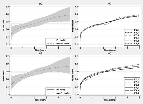
Table 1. Agreement of AIC and BIC with SKL for different models on the log cumulative hazard scale.

		AIC										BIC
		3,1	3,3	5,1	5,3	5,5	7,1	7,3	7,5	7,7	Total	3,1	3,3	5,1	5,3	5,5	7,1	7,3	7,5	7,7	Total
Scenario 1; SKL	3,1	341	45	43	4	9	32	2	2	3	481	480	1	0	0	0	0	0	0	0	481
	3,3	4	0	1	0	1	1	0	0	0	7	7	0	0	0	0	0	0	0	0	7
	5,1	11	1	0	0	0	0	0	0	0	12	12	0	0	0	0	0	0	0	0	12
	5,3	0	0	0	0	0	0	0	0	0	0	0	0	0	0	0	0	0	0	0	0
	5,5	0	0	0	0	0	0	0	0	0	0	0	0	0	0	0	0	0	0	0	0
	7,1	0	0	0	0	0	0	0	0	0	0	0	0	0	0	0	0	0	0	0	0
	7,3	0	0	0	0	0	0	0	0	0	0	0	0	0	0	0	0	0	0	0	0
	7,5	0	0	0	0	0	0	0	0	0	0	0	0	0	0	0	0	0	0	0	0
	7,7	0	0	0	0	0	0	0	0	0	0	0	0	0	0	0	0	0	0	0	0
	Total	356	46	44	4	10	33	2	2	3	500	499	1	0	0	0	0	0	0	0	500
Scenario 2; SKL	3,1	0	0	0	0	0	0	0	0	0	0	0	0	0	0	0	0	0	0	0	0
	3,3	0	0	0	0	0	0	2	0	0	2	0	0	1	0	0	0	1	0	0	2
	5,1	0	0	0	0	0	0	0	0	0	0	0	0	0	0	0	0	0	0	0	0
	5,3	0	0	0	1	4	0	45	74	13	137	0	2	1	57	9	1	64	3	0	137
	5,5	0	0	0	3	4	1	147	70	15	240	0	2	11	114	0	6	106	1	0	240
	7,1	0	0	0	0	0	0	0	0	0	0	0	0	0	0	0	0	0	0	0	0
	7,3	0	0	0	2	3	0	6	12	4	27	0	0	1	16	4	0	6	0	0	27
	7,5	0	0	0	10	3	0	45	19	7	84	0	1	3	66	0	0	13	1	0	84
	7,7	0	0	0	2	0	0	4	4	0	10	0	0	1	7	0	0	2	0	0	10
	Total	0	0	0	18	14	1	249	179	39	500	0	5	18	260	13	7	192	5	0	500
Scenario 3; SKL	3,1	0	0	0	0	0	0	0	0	0	0	0	0	0	0	0	0	0	0	0	0
	3,3	0	1	0	0	5	0	0	1	3	10	2	1	0	0	7	0	0	0	0	10
	5,1	0	0	0	0	0	0	0	0	0	0	0	0	0	0	0	0	0	0	0	0
	5,3	0	0	0	0	1	0	0	0	0	1	0	0	0	0	1	0	0	0	0	1
	5,5	1	54	0	11	284	0	5	46	20	421	109	282	1	1	28	0	0	0	0	421
	7,1	0	0	0	0	0	0	0	0	0	0	0	0	0	0	0	0	0	0	0	0
	7,3	0	0	0	0	0	0	0	0	0	0	0	0	0	0	0	0	0	0	0	0
	7,5	0	9	0	2	51	0	0	0	3	65	18	46	0	0	1	0	0	0	0	65
	7,7	0	1	0	0	2	0	0	0	0	3	0	3	0	0	0	0	0	0	0	3
	Total	1	65	0	13	343	0	5	47	26	500	129	332	1	1	37	0	0	0	0	500

It is not clear how many degrees of freedom are required to capture the shape of this time-dependent effect, or the baseline function in this non-proportional hazards model. Note that we write a, b degrees of freedom to denote a degrees of freedom to capture the baseline hazard and b degrees of freedom to model the time-dependent effect. Figure 1b and d presents the predicted hazard ratios (most deprived versus least deprived) from flexible parametric survival models on the log cumulative hazard scale and log hazard scale respectively with different degrees of freedom; see the figure legends for the different models fitted. Note that a spline function with one degree of freedom is simply a linear function of log time. Although all of the predicted hazard ratios capture a similar shape, a general increase over time, there are some differences between the curves. It is not clear which of the models better captures the true hazard ratio. To aid selection of the degrees of freedom, the AIC and BIC can be calculated. On the log hazard scale both criteria suggested the model with 7 and 1 degrees of freedom provided the better fit. However, on the log cumulative hazard scale the AIC suggested that the model with 5 degrees of freedom to model the baseline and 1 degree of freedom for the deviation in the time-dependent effect respectively had the better fit, whereas the BIC suggested that the model with 3 and 1 degrees of freedom was the better model. This inconsistency on the log cumulative hazard scale highlights a problem with using these model selection criteria; it is of interest to determine whether one criterion outperforms the other. A simulation setting allows us to know the true function, thus we use this approach to assess restricted cubic splines in capturing biologically plausible time-dependent effects across a range of scenarios.

2.4. Simulation strategy

A simulation study was undertaken where the true non-proportional hazard functions were known in order to assess the fit of the restricted cubic splines implemented within non-proportional flexible parametric survival models on the log cumulative hazard scale and on the log hazard scale, and to assess the performance of model selection using the AIC and the BIC.

2.4.1. Simulation design and data generation

Five hundred datasets were simulated using both sample sizes of 1 000 and 10 000; results are only presented here for sample size 1 000. Survival times in years were simulated on the hazard scale from a mixture Weibull distributions alongside a time-dependent effect of covariate x. The covariate x was binary and generated from a Bernoulli(0.5) distribution. Simulated survival times were implemented using software available in Stata (Crowther and Lambert 2012) using the method proposed by Bender et al. (Bender, Augustin, and Blettner 2005) and extended by Crowther and Lambert (Crowther and Lambert 2013). Administrative censoring was applied at five years.

2.4.2. Simulation scenarios

Nine scenarios were simulated using combinations from three baseline Weibull distributions and three time-dependent effect functions; three out of the nine scenarios are presented here. The baseline distributions were similar to Weibull and mixture Weibull distributions used by Rutherford et al. (Rutherford, Crowther, and Lambert 2015). The time-dependent functions were based upon time-dependent effects found in datasets and previous studies to ensure that both complex and biologically plausible effects were simulated; the survival, hazard and log hazard ratio of the simulation scenarios are shown in Figure 2. Note that spline functions were not used to create the underlying true model. The time-dependent effect used within scenario 1 was based upon the time-dependent effect seen in England and Wales breast cancer data described previously. Thus, scenario 1 had a log hazard ratio which was a function of log time. The time-dependent effect used within scenario 2 had a log hazard ratio with a turning point. This pattern was based upon a hazard ratio seen between stages of colon carcinoma patients diagnosed in Finland (Lambert et al. 2007). The time-dependent effect used within scenario 3 was based upon a time-dependent effect used within a simulation study by Abrahamowicz et al. (Abrahamowicz, MacKenzie, and Esdaile 1996); in this study quadratic splines struggled to capture the shape of this time-dependent effect. Further details on the simulated scenarios are available in Table 2 of the Supplementary Materials.

Figure 2. Survival proportions, hazard rates and log hazard ratios of the three simulated scenarios.

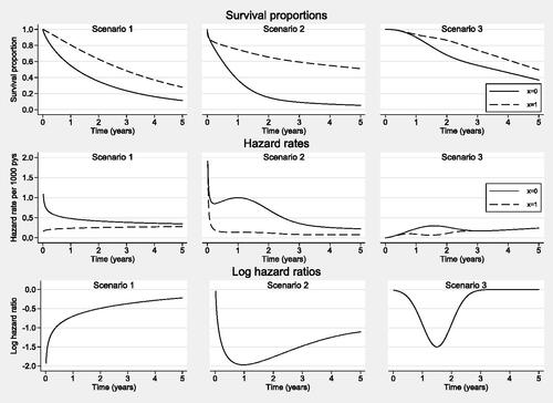
Table 2. Agreement of AIC and BIC with SKL for different models on the log hazard scale.

		AIC										BIC
		3,1	3,3	5,1	5,3	5,5	7,1	7,3	7,5	7,7	Total	3,1	3,3	5,1	5,3	5,5	7,1	7,3	7,5	7,7	Total
Scenario 1; SKL	3,1	338	46	50	8	8	18	4	2	3	477	476	1	0	0	0	0	0	0	0	477
	3,3	6	0	2	0	1	1	0	0	0	10	10	0	0	0	0	0	0	0	0	10
	5,1	10	3	0	0	0	0	0	0	0	13	13	0	0	0	0	0	0	0	0	13
	5,3	0	0	0	0	0	0	0	0	0	0	0	0	0	0	0	0	0	0	0	0
	5,5	0	0	0	0	0	0	0	0	0	0	0	0	0	0	0	0	0	0	0	0
	7,1	0	0	0	0	0	0	0	0	0	0	0	0	0	0	0	0	0	0	0	0
	7,3	0	0	0	0	0	0	0	0	0	0	0	0	0	0	0	0	0	0	0	0
	7,5	0	0	0	0	0	0	0	0	0	0	0	0	0	0	0	0	0	0	0	0
	7,7	0	0	0	0	0	0	0	0	0	0	0	0	0	0	0	0	0	0	0	0
	Total	354	49	52	8	9	19	4	2	3	500	499	1	0	0	0	0	0	0	0	500
Scenario 2; SKL	3,1	0	0	0	0	0	0	0	0	0	0	0	0	0	0	0	0	0	0	0	0
	3,3	0	0	0	3	1	0	8	7	57	76	0	0	5	21	4	5	36	1	4	76
	5,1	0	0	0	0	0	0	0	0	0	0	0	0	0	0	0	0	0	0	0	0
	5,3	0	0	0	0	6	0	30	54	150	240	1	10	8	80	23	15	94	1	8	240
	5,5	0	0	0	4	3	0	68	3	41	119	1	9	8	62	0	7	32	0	0	119
	7,1	0	0	0	0	0	0	0	0	0	0	0	0	0	0	0	0	0	0	0	0
	7,3	0	0	0	2	16	0	10	5	15	48	1	6	5	33	3	0	0	0	0	48
	7,5	0	0	0	3	1	0	7	0	4	15	0	2	2	11	0	0	0	0	0	15
	7,7	0	0	0	0	0	0	2	0	0	2	0	0	1	1	0	0	0	0	0	2
	Total	0	0	0	12	27	0	125	69	267	500	3	27	29	208	30	27	162	2	12	500
Scenario 3; SKL	3,1	0	0	0	0	0	0	0	0	0	0	0	0	0	0	0	0	0	0	0	0
	3,3	0	2	0	0	15	0	0	6	4	27	7	15	0	1	4	0	0	0	0	27
	5,1	0	0	0	0	0	0	0	0	0	0	0	0	0	0	0	0	0	0	0	0
	5,3	0	0	0	0	0	0	0	0	1	1	0	1	0	0	0	0	0	0	0	1
	5,5	1	60	0	1	133	0	6	45	53	299	91	189	0	3	16	0	0	0	0	299
	7,1	0	0	0	0	0	0	0	0	0	0	0	0	0	0	0	0	0	0	0	0
	7,3	0	1	0	0	0	0	0	0	0	1	1	0	0	0	0	0	0	0	0	1
	7,5	0	7	0	1	42	0	0	3	12	65	18	43	0	1	3	0	0	0	0	65
	7,7	0	28	0	5	63	0	0	6	5	107	35	69	0	2	1	0	0	0	0	107
	Total	1	98	0	7	253	0	6	60	75	500	152	317	0	7	24	0	0	0	0	500

2.4.3. Analyses of simulated data

Flexible parametric survival models were fitted to each simulated dataset both on the log cumulative hazard and log hazard scale with varying degrees of freedom. Three, five and seven degrees of freedom were used to model the baseline and one, three, five and seven degrees of freedom to model the time-dependent effect. The degrees of freedom for the time-dependent effect were limited to less than or equal to the number of degrees of freedom for the baseline effect since in practice one would rarely fit a model with more parameters for the time-dependent effect than the baseline. The time-dependent log hazard ratio, and hazard and survival functions for both x = 0 and x = 1 were predicted from each model and compared to their respective true value in order to calculate the bias and coverage of each estimate; these were evaluated at one, three and five years. Coverage was calculated as the percentage of the confidence intervals, estimated from each model in every simulated dataset, that contained the true value. Root mean squared error (rMSE) estimates were also calculated in order to give a reflection of the variance of the estimates. The AIC, the BIC and the SKL were calculated for each fitted model and the optimal degrees of freedom suggested by each criteria compared.

3. Results

The average number of events were 803.2, 722.1 and 567.8 for scenarios 1, 2 and 3 respectively for sample size 1 000 over 5 years of follow-up. Convergence of models was high; 100% of all models on the log cumulative hazard scale converged and at least 98.9% of models on the log hazard scale converged in each scenario. Figures 3–5 present the bias in predictions of the survival, hazard function and log hazard ratios at one, three and five years for different degrees of freedom on each of the modeling scales for the three scenarios. Figures showing the rMSE can be found in Figures 3–5 of the Supplementary Materials.

Figure 3. Bias in the survival proportions, from models on the log cumulative hazard, log(H), and log hazard, log(h), scales with different degrees of freedom. Sample size 1 000. Mean values based on 500 simulations.

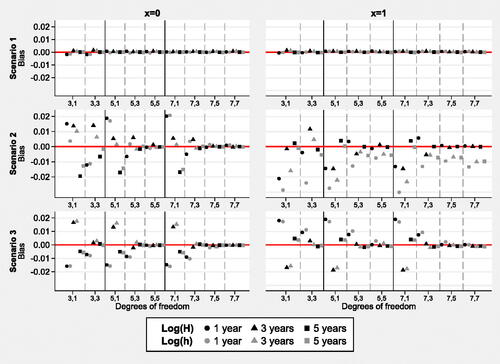
Figure 4. Bias in the hazard rates from models on the log cumulative hazard, log(H), and log hazard, log(h), scales with different degrees of freedom. Sample size 1 000. Mean values based on 500 simulations.

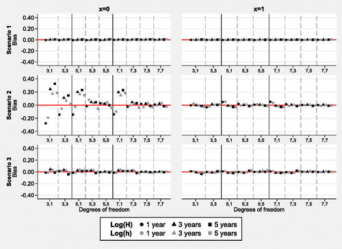
Figure 5. Bias in the survival proportions log hazard ratios from models on the log cumulative hazard, log(H), and log hazard, log(h), scales with different degrees of freedom. Sample size 1 000. Mean values based on 500 simulations.

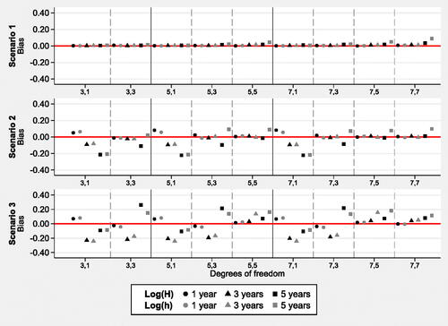
In scenario 1, the simplest of all the scenarios, negligible bias was found in the survival estimates over all degrees of freedom; absolute bias in the survival proportion was below 0.002. Very little bias was seen in the hazard rates and log hazard ratios. Larger bias was seen in models on the log hazard scale at time five as the time-dependent degrees of freedom increased, indicating potential over-modeling on this scale with larger degrees of freedom. Similar patterns were seen in the rMSE estimates. Very low values were seen in models with fewer degrees of freedom and increased rMSE values were seen in more complex models where it is possible that over-modeling had occurred.

Scenario 2 was more complex and had larger amounts of bias for low degrees of freedom. Bias was particularly large in hazard estimates and log hazard ratio estimates; this noticeably decreased as more degrees of freedom were chosen to model the deviation in the time-dependent effect. This pattern was also evident in the survival estimates. Absolute bias in the survival estimates was lower than 0.007 for models on the log cumulative hazard scale with at least 5 degrees of freedom to model the baseline hazard and at least 3 degrees of freedom to model the deviation from the baseline in the time-dependent effect. Absolute bias in survival estimates was generally higher when modeling on the log hazard scale, although this was approximately 0.01 or less if at least 7,5 degrees of freedom were specified. The rMSE estimates indicated that more variation was seen in the estimates for scenario 2 than 1 and 3. The rMSE values were similar in models with more than 5,5 degrees of freedom; lower rMSE estimates were generally seen on the log cumulative hazard scale.

The bias in scenario 3 was low for all survival estimates and approximately zero for some. The bias for the hazard and log hazard ratio estimates decreased as larger degrees of freedom were specified. Absolute bias in the survival estimates was less than or equal to 0.001 for models on the log cumulative hazard scale with at least 5 degrees of freedom to model the baseline hazard and to model the deviation from the baseline in the time-dependent effect. Absolute bias in survival estimates was less than 0.003 when modeling on the log hazard scale provided 5 degrees of freedom or more were specified to model the deviation in the time-dependent effect. The rMSE estimates suggested that variation was low in the survival and hazard estimates; larger rMSE estimates were seen in the log hazard ratio estimates especially in models with 1 degree of freedom to model the time-dependent effect. Bias was marginally higher when modeling on the log hazard scale. Coverage for all scenarios was close to 95%, the more complex scenarios required larger degrees of freedom to obtain this coverage.

Table 1 shows the agreement between the optimal models selected by the SKL and the AIC, and the SKL and the BIC for models on the log cumulative hazard scale. In scenario 1 with sample size 1 000, the SKL selected the model with 3,1 degrees of freedom 481 times out of 500 replications as being the optimal model. The AIC and the BIC suggested the same model 356 and 499 times respectively. The SKL selected a larger variety of optimal models in scenario 2; the model with 5,5 degrees of freedom was chosen as optimal in approximately half of the datasets. The AIC generally suggested more complicated models and BIC suggested simpler models. The optimal model selected most frequently by the SKL in scenario 3 was the model with 5,5 degrees of freedom. The AIC suggested this as the optimal model the majority of the time whilst the BIC suggested models which were too simple in the majority of replications. Results for all three scenarios were similar when modeling the log hazard, see Table 2, or the log cumulative hazard and were in agreement with the models which showed the lowest bias.

4. Discussion

We undertook this simulation study to better understand the impact of user-selected degrees of freedom in flexible parametric survival models implemented in applied studies. The results presented indicate that restricted cubic splines accurately capture time-dependent effects if appropriate degrees of freedom are selected; these results are consistent with the findings of Rutherford et al. (Rutherford, Crowther, and Lambert 2015) for proportional-hazards models. Bias was higher in models with lower degrees of freedom since these models were unable to capture the underlying complexity of the functions. However, survival estimates were fairly insensitive to an inappropriate number of degrees of freedom specified for the baseline hazard and the time-dependent effect. Models with many degrees of freedom produced slight biases due to over-modeling by capturing too much random variation in the observed data, however, these effects were smaller than those found when under-modeling since the inclusion of time-dependent effects increases the complexity of the data. Models on the log cumulative hazard scale and the log hazard scale captured hazard functions similarly well, although different degrees of freedom were optimal in some scenarios. A well fitting model was found for all scenarios on both scales. Neither the AIC nor the BIC consistently performed better than the other, however, the BIC selected too simple models in scenario 3; it is important to remember that the time-dependent effect selected for scenario 3 was artificial and thus the largest challenge for the splines. Other than this, both the AIC and BIC suggested optimal models with low bias which is reassuring when conducting applied research.

Since the hazard function is inherently more complex than the cumulative hazard function, more degrees of freedom may be required when modeling on the log hazard scale. Also, over-modeling was more apparent on the log hazard scale in the simplest scenario, 1. This scenario, due to its simplicity, did not require many degrees of freedom and bias was larger when a model was fitted with a large number of degrees of freedom to model the deviation in the time-dependent effect. The computation time was also different due to the need for numerical integration when modeling on the log hazard scale. However, the computation time taken to model on the log hazard scale in a single dataset is less problematic than the many models fitted in a simulation study.

Due to the complexity of some of the scenarios, accurately capturing the underlying hazards were problematic due to a small sample size. This was particularly clear when considering the BIC in scenario 3. The BIC suggested the two simplest models as optimal the majority of the time where bias was large. When the sample size was increased to 10 000 (results not shown) the BIC suggested more complex models which resulted in lower bias. The results in this paper indicate that neither the AIC nor BIC out-perform the other in all situations; unfortunately this conclusion is not helpful for real data analyses. There has been evidence that one or the other criterion perform better in different situations (Emiliano, Vivanco, and de Menezes 2014; Burnham and Anderson 2004). Emphasis is put on the AIC and BIC here since these are the most widely used in practice, and thus we were interested in determining whether there was a clear advantage in using one over the other, however, there are other information criteria which may be useful in other situations (Spiegelhalter et al. 2002; Ishiguro, Sakamoto, and Kitagawa 1997; Wei 1992; Konishi and Kitagawa 1996). Our results suggest that relying on one criterion in this context is not advisable, instead both should be used for guidance. One possible alternative to selecting a model by use of information criteria is to make inferences based on an averaged model (Hoeting et al. 1999; Burnham and Anderson 2002).

Although the functions for the time-dependent effect considered in the simulations were of varying complexity, reality may still be more complex than considered in this study due to the consideration of only one binary time-dependent effect. This simplistic analysis is a useful starting point, but further assessment under more complex multivariate analyses should be an extension of this work. An additional extension would be to also consider non-linear effects of predictors on the log hazard since there is evidence that not allowing for non-linear effects can result in bias under non-proportionality (Abrahamowicz and MacKenzie 2007; Sauerbrei, Royston, and Look 2007); these can easily be introduced by modeling covariates continuously using restricted cubic splines. These additional complexities would contribute to a more complete assessment since they may be more similar to those seen in practice. We also only consider flexible parametric survival models to capture time-dependent effects. Outside of the fully parametric framework, there are several alternative approaches to modeling non-proportional hazards, including estimation using penalized or restricted maximum likelihood (Gu 2013). These alternatives may be advantageous when modeling for multiple smooth terms. A comparison of these methods with the flexible parametric survival approach would make for interesting further research.

The greatest advantage of flexible parametric survival models is that their use of restricted cubic splines make them flexible and one can include time-dependent effects simply in the models. They are also easily implemented for relative survival (Nelson et al. 2007) and for modeling cure (Andersson et al. 2014); the results in this study also apply within these frameworks.

Our motivating example illustrates one of the problems with using the AIC and BIC, that each information criterion can select a different model. Although one final model should be chosen in practice, we believe it is a strength to be able to show results are not sensitive to model choices via sensitive analyses. We present such a sensitivity analysis in Figures 1 and 2 of the Supplementary Materials where we compare the survival proportions and hazard ratios from different models fitted to the motivating example dataset. Different degrees of freedom resulted in small changes on the hazard ratio scale, but made very little difference to the survival estimates. The hazard ratio estimated from more complex models fluctuated a little over the five years of follow-up. It seems unlikely that hazard ratio predicted from the model with, for example, 7,5 degrees of freedom on the log hazard scale, is the true hazard ratio due to these fluctuations, and is more likely an artifact of the complex model. In this motivating example, we would have suggested to select the model with 7,1 degrees of freedom on the log hazard scale (where the AIC and BIC agreed). On the log cumulative hazard scale we would have selected the model with 5,1 degrees of freedom (chosen by the AIC) and been happy that 1) 5 degrees of freedom is most likely flexible enough to accurately capture the effect (Syriopoulou et al. 2019), and 2) that both point estimates and uncertainty were almost identical to the model chosen by the BIC (3,1 degrees of freedom).

4.1. Advice for users of flexible parametric survival models

We have presented a simulation study where it has been possible to identify the best model in terms of the lowest SKL. However, when faced with a single data set such an approach cannot be used as the true function is unknown. A key result from our simulation study is that provided there are sufficient degrees of freedom the bias in the estimated survival, hazard functions and time-dependent log hazard ratios is small. We tend to deal with fairly large datasets with several thousand observations. Our usual starting point is to use 5 degrees of freedom for the baseline and 3 degrees of freedom for any time-dependent effects. This is likely to capture most complex shapes. We would then inspect the AIC and BIC for a selection of models with more and less degrees of freedom to see if we had strong evidence of needing a more simple or more complex model. However, when comparing models we would always compare the key quantity we were interested in estimating. For example, by comparing the hazard ratio as shown in the motivating example, or other measures such as the age standardized survival (Lambert, Dickman, and Rutherford 2015), a time-dependent hazard ratio (Lambert et al. 2011) or the loss in expectation of life (Andersson et al. 2015; Bower, Crowther, and Lambert 2016). We see these comparisons as more important than just a comparison of the AIC or BIC since it is a strength to be able to state that conclusions of the analysis do not change when different reasonable models are chosen.

4.2. Conclusions

Restricted cubic splines accurately capture simple and complex time-dependent effects provided suitable degrees of freedom are chosen to allow an appropriate flexibility. If interest lies in survival estimates then model misspecification should not be too problematic. It should always be possible for an analyst to identify a well fitting model when modeling on the log cumulative hazard scale or on the log hazard scale. The AIC and BIC should be calculated to guide users towards appropriate degrees of freedom but one or the other should not be relied upon to select the ‘correct’ model. Instead, users should perform sensitivity analyses, such as those conducted in Figure 1b and d, and remember that many models will likely fit the data well.

Disclosure statement

The authors have declared no conflict of interest.

Additional information

Funding

Michael J. Crowther was in part funded by a National Institute for Health Research (NIHR) Doctoral Research Fellowship [DRF-2012-05-409]. Therese M-L. Andersson was supported by the Swedish Research Council [521-2011-3205] and the Swedish E-Science Research Center. Paul C. Lambert was supported the Swedish Research Council [521-2013-3383] and the Swedish Cancer Society [CAN2012/75Y]. Mark Clements was supported by the Swedish Cancer Society [CAN2012/765]. Swedish Research Council (Vetenskapsrådet in Swedish), Swedish Cancer Society (Cancerfonden in Swedish).

References

- Abrahamowicz, M., and T. A. MacKenzie. 2007. Joint estimation of time-dependent and non-linear effects of continuous covariates on survival. Statistics in Medicine 26 (2):392–408. doi:https://doi.org/10.1002/sim.2519.
- Abrahamowicz, M., T. MacKenzie, and J. M. Esdaile. 1996. Time-dependent hazard ratio: Modeling and hypothesis testing with application in lupus nephritis. Journal of the American Statistical Association 91 (436):1432–9. doi:https://doi.org/10.2307/2291569.
- Akaike, H. 1973. Information theory as an extension of the maximum likelihood principle. In Second International Symposium on Information Theory, ed. B. N. Petrov and F. Csaki, 267–281, Budapest: Akademiai Kiado.
- Andersson, T. M.-L., H. Eriksson, J. Hansson, E. Månsson-Brahme, P. W. Dickman, S. Eloranta, M. Lambe, and P. C. Lambert. 2014. Estimating the cure proportion of malignant melanoma, an alternative approach to assess long term survival: A population-based study. Cancer Epidemiology 38 (1):93–9. doi:https://doi.org/10.1016/j.canep.2013.12.006.
- Andersson, T. M.-L., P. W. Dickman, S. Eloranta, A. Sjövall, M. Lambe, and P. C. Lambert. 2015. The loss in expectation of life after colon cancer: A population-based study. BMC Cancer 15 (1):412 doi:https://doi.org/10.1186/s12885-015-1427-2.
- Andersson, T. M.-L., P. W. Dickman, S. Eloranta, and P. C. Lambert. 2011. Estimating and modelling cure in population-based cancer studies within the framework of flexible parametric survival models. BMC Medical Research Methodology 11 (1):96. doi:https://doi.org/10.1186/1471-2288-11-96.
- Bender, R., T. Augustin, and M. Blettner. 2005. Generating survival times to simulate Cox proportional hazards models. Statistics in Medicine 24 (11):1713–23. doi:https://doi.org/10.1002/sim.2059.
- Bower, H., M. J. Crowther, and P. Lambert. 2016. strcs: A command for fitting flexible parametric survival models on the log-hazard scale. The Stata Journal: Promoting Communications on Statistics and Stata 16 (4):989–1012. doi:https://doi.org/10.1177/1536867X1601600410.
- Bower, H., T. M. L. Andersson, M. Bjorkholm, P. W. Dickman, P. C. Lambert, and A. R. Derolf. 2016. Continued improvement in survival of acute myeloid leukemia patients: An application of the loss in expectation of life. Blood Cancer Journal 6 (2):e390.
- Burnham, K. P., and D. R. Anderson. 2002. Model selection and multimodel inference: A practical information-theoretic approach. New York: Springer.
- Burnham, K. P., and D. R. Anderson. 2004. Multimodel inference: Understanding AIC and BIC in model selection. Sociological Methods and Research 33 (2):261–304. doi:https://doi.org/10.1177/0049124104268644.
- Carstairs, V., and R. Morris. 1991. Deprivation and health in Scotland. Aberdeen: Aberdeen University Press.
- Coleman, M. P., P. Babb, P. Damiecki, P. Grosclaude, S. Honjo, J. Jones, G. Knerer, A. Pitard, M. Quinn, A. Sloggett, and B. De Stavola. 1999. Cancer survival trends in England and Wales, 1971–1995: Deprivation and NHS region. No. 61 in Studies in Medical and Population Subjects, London: The Stationery Office.
- Colzani, E., A. Liljegren, A. L. V. Johansson, J. Adolfsson, H. Hellborg, P. F. L. Hall, and K. Czene. 2011. Prognosis of patients with breast cancer: Causes of death and effects of time since diagnosis, age, and tumor characteristics. Journal of Clinical Oncology 29 (30):4014–21. doi:https://doi.org/10.1200/JCO.2010.32.6462.
- Cox, D. R. 1972. Regression models and life-tables (with discussion). JRSSB 34:187–220. doi:https://doi.org/10.1111/j.2517-6161.1972.tb00899.x.
- Crowther, M. J., and P. C. Lambert. 2012. Simulating complex survival data. The Stata Journal: Promoting Communications on Statistics and Stata 12 (4):674–87. doi:https://doi.org/10.1177/1536867X1201200407.
- Crowther, M. J., and P. C. Lambert. 2013. Simulating biologically plausible complex survival data. Statistics in Medicine 32 (23):4118–34. doi:https://doi.org/10.1002/sim.5823.
- Crowther, M. J., and P. C. Lambert. 2013. stgenreg: A Stata package for general parametric survival analysis. Journal of Statistical Software 53 (12):1–17. doi:https://doi.org/10.18637/jss.v053.i12.
- Crowther, M. J., and P. C. Lambert. 2014. A general framework for parametric survival analysis. Statistics in Medicine 33 (30):5280–97. doi:https://doi.org/10.1002/sim.6300.
- Crowther, M. J., M. P. Look, and R. D. Riley. 2014. Multilevel mixed effects parametric survival models using adaptive gauss-hermite quadrature with application to recurrent events and individual participant data meta-analysis. Statistics in Medicine 33 (22):3844–58. doi:https://doi.org/10.1002/sim.6191.
- Durrleman, S., and R. Simon. 1989. Flexible regression models with cubic splines. Statistics in Medicine 8 (5):551–61. doi:https://doi.org/10.1002/sim.4780080504.
- Emiliano, P., M. J. Vivanco, and F. S. de Menezes. 2014. Information criteria: How do they behave in different models? Computational Statistics & Data Analysis 69:141–53. doi:https://doi.org/10.1016/j.csda.2013.07.032.
- Grambsch, P. M., and T. M. Therneau. 1994. Proportional hazards tests and diagnostics based on weighted residuals. Biometrika 81 (3):515–26. doi:https://doi.org/10.2307/2337123.
- Gray, R. J. 1992. Flexible methods for analyzing survival data using splines, with applications to breast cancer prognosis. Journal of the American Statistical Association 87 (420):942–51. doi:https://doi.org/10.2307/2290630.
- Gu, C. 2013. Smoothing spline ANOVA models. 2nd ed. New York: Springer.
- Hastie, T. J., and R. J. Tibshirani. 1993. Varying-coefficient models. Journal of the Royal Statistical Society (Series B) 55:757–96. doi:https://doi.org/10.1111/j.2517-6161.1993.tb01939.x.
- Hernán, M. A. 2010. The hazards of hazard ratios. Epidemiology (Cambridge, Mass.) 21(1):13–5. doi:https://doi.org/10.1097/EDE.0b013e3181c1ea43.
- Hoeting, J. A., D. Madigan, A. E. Raftery, and C. T. Volinsky. 1999. Bayesian model averaging: A tutorial. Statistical Science 14:382–401. doi:https://doi.org/10.1214/ss/1009212814.
- Ishiguro, M., Y. Sakamoto, and G. Kitagawa. 1997. Bootstrapping log likelihood and EIC, an extention of AIC. Annals of the Institute of Statistical Mathematics 49 (3):411–34. doi:https://doi.org/10.1023/A:1003158526504.
- Jatoi, I., W. F. Anderson, J.-H. Jeong, and C. K. Redmond. 2011. Breast cancer adjuvant therapy: Time to consider its time-dependent effects. Journal of Clinical Oncology 29 (17):2301–4. doi:https://doi.org/10.1200/JCO.2010.32.3550.
- Kandala, N.-B., M. Connock, R. Pulikottil-Jacob, P. Sutcliffe, M. J. Crowther, A. Grove, H. Mistry, and A. Clarke. 2015. Setting benchmark revision rates for total hip replacement: Analysis of registry evidence. BMJ 350 (mar09 1):h756. doi:https://doi.org/10.1136/bmj.h756.
- King, N. B., S. Harper, and M. E. Young. 2012. Use of relative and absolute effect measures in reporting health inequalities: Structured review. BMJ 345 (sep03 1):e5774. doi:https://doi.org/10.1136/bmj.e5774.
- Konishi, S., and G. Kitagawa. 1996. Generalised information criteria in model selection. Biometrika 83 (4):875–90. doi:https://doi.org/10.1093/biomet/83.4.875.
- Kullback, S., and R. A. Leibler. 1951. On information and sufficiency. The Annals of Mathematical Statistics 22 (1):79–86. doi:https://doi.org/10.1214/aoms/1177729694.
- Lambert, P. C., and P. Royston. 2009. Further development of flexible parametric models for survival analysis. The Stata Journal: Promoting Communications on Statistics and Stata 9 (2):265–90. doi:https://doi.org/10.1177/1536867X0900900206.
- Lambert, P. C., L. Holmberg, F. Sandin, F. Bray, K. M. Linklater, A. Purushotham, D. Robinson, and H. Møller. 2011. Quantifying differences in breast cancer survival between England and Norway. Cancer Epidemiology 35 (6):526–33.
- Lambert, P. C., P. W. Dickman, and M. J. Rutherford. 2015. Comparison of approaches to estimating age-standardized net survival. BMC Medical Research Methodology 15:64.
- Lambert, P. C., P. W. Dickman, P. Österlund, T. M.-L. Andersson, R. Sankila, and B. Glimelius. 2007. Temporal trends in the proportion cured for cancer of the colon and rectum: A population-based study using data from the Finnish cancer registry. International Journal of Cancer 121 (9):2052–9. doi:https://doi.org/10.1002/ijc.22948.
- McMinn, D. J. W., K. I. E. Snell, J. Daniel, R. B. C. Treacy, P. B. Pynsent, and R. D. Riley. 2012. Mortality and implant revision rates of hip arthroplasty in patients with osteoarthritis: Registry based cohort study. BMJ 344 (jun14 1):e3319. doi:https://doi.org/10.1136/bmj.e3319.
- Nelson, C. P., P. C. Lambert, I. B. Squire, and D. R. Jones. 2007. Flexible parametric models for relative survival, with application in coronary heart disease. Statistics in Medicine 26 (30):5486–98. doi:https://doi.org/10.1002/sim.3064.
- Pawitan, Y. 2001. In all likelihood – statistical modelling and inference using likelihood. Oxford: Oxford University Press.
- Royston, P., and M. K. B. Parmar. 2002. Flexible parametric proportional-hazards and proportional-odds models for censored survival data, with application to prognostic modelling and estimation of treatment effects. Statistics in Medicine 21 (15):2175–97. doi:https://doi.org/10.1002/sim.1203.
- Royston, P., and P. C. Lambert. 2011. Flexible parametric survival analysis in Stata: Beyond the cox model. College Station, TX: Stata Press.
- Rutherford, M. J., M. J. Crowther, and P. C. Lambert. 2015. The use of restricted cubic splines to approximate complex hazard functions in the analysis of time-to-event data: A simulation study. Journal of Statistical Computation and Simulation 85 (4):777–93. doi:https://doi.org/10.1080/00949655.2013.845890.
- Sauerbrei, W., P. Royston, and M. Look. 2007. A new proposal for multivariable modelling of time-varying effects in survival data based on fractional polynomial time-transformation. Biometrical Journal 49 (3):453–73. doi:https://doi.org/10.1002/bimj.200610328.
- Schwarz, G. 1978. Estimating the dimension of a model. The Annals of Statistics 6 (2):461–4. doi:https://doi.org/10.1214/aos/1176344136.
- Smith, A. J., P. Dieppe, K. Vernon, M. Porter, and A. W. Blom. 2012. Failure rates of stemmed metal-on-metal hip replacements: Analysis of data from the national joint registry of England and Wales. The Lancet 379 (9822):1199–204. doi:https://doi.org/10.1016/S0140-6736(12)60353-5.
- Spiegelhalter, D. J., N. G. Best, B. P. Carlin, and A. van der Linde. 2002. Bayesian measures of model complexity and fit. Journal of the Royal Statistical Society: Series B (Statistical Methodology) 64 (4):583–639. doi:https://doi.org/10.1111/1467-9868.00353.
- Syriopoulou, E., S. I. Mozumder, M. J. Rutherford, and P. C. Lambert. 2019. Robustness of individual and marginal model-based estimates: A sensitivity analysis of flexible parametric models. Cancer Epidemiology 58:17–24.
- Wei, C. Z. 1992. On predictive least squares principles. The Annals of Statistics 20 (1):1–42. doi:https://doi.org/10.1214/aos/1176348511.
- Wynant, W., and M. Abrahamowicz. 2015. Flexible estimation of survival curves conditional on non-linear and time-dependent predictor effects. Statistics in Medicine 35 (4):553–565. pp. n/a–n/a, SIM-15-0238.R1. doi:https://doi.org/10.1002/sim.6740.