The t linear mixed model: model formulation, identifiability and estimation

Abstract

The robustness of the t linear mixed model (tLMM) has been proved and exploited in many applications. Various publications emerged with the aim of proving superiority with respect to traditional linear mixed models, extending to more general settings and proposing more efficient estimation methods. However, little attention has been paid to the mathematical properties of the model itself and to the evaluation of the proposed estimation methods. In this paper we perform an in-depth analysis of the tLMM, evaluating a direct maximum likelihood estimation method via an intensive simulation study and investigating some identifiability properties. The theoretical findings are illustrated through an application to a dataset collected from a sleep trial.

Keywords:

• Heterogeneous variances
• Latent variable
• Model identifiability
• Outliers
• Variance components

1. Introduction

Linear mixed models (LMM) are widely popular for their appealing feature of modeling both the intra- and inter-subject variability with a broad set of possible correlation structures (Laird and Ware 1982). However, they rely on normality assumptions, and can be very sensitive to outlying data and heavy tails distributions. The multivariate t distribution (see the publication of Kotz and Nadarajah (2004) for a comprehensive discussion of its characterizations and properties) has been proposed to make linear regression and mixed linear regression robust (Lange, Little, and Taylor 1989; Pinheiro, Liu, and Wu 2001). In particular, the t linear mixed model (tLMM) is a natural extension of the classical LMM in which the response variable is jointly t distributed (Pinheiro, Liu, and Wu 2001). A convenient hierarchical formulation of the tLMM can be derived by mixing the multivariate normal distribution of the response variable with a gamma-distributed latent scaling variable for the covariance matrix (Pinheiro, Liu, and Wu 2001). This characteristic makes the tLMM robust to heavy tails distributions of the observed data, and thus more appropriate than the LMM when normality assumptions are violated. Furthermore, the tLMM is a favorable choice over other robust methods because robustness is achieved with only one extra parameter compared to traditional LMMs, and the model structure allows the analysis of random variances.

In fact, many authors have explored applications and extensions of the tLMM, and the related literature is quite broad.

A similar model has been proposed to analyze heterogeneous within-subject variances (Chinchilli, Esinhart, and Miller 1995). Here the authors made no distributional assumptions on the random effects, while they imposed a similar hierarchical structure for the residual variances. Chinchilli, Esinhart, and Miller (1995) aimed at studying the within-subject variability of two different laboratory techniques, treated consequently the fixed effects as nuisance parameters, and proposed partial likelihood estimation for a model with only random intercept and no covariates. An extension of this model has been introduced for the analysis of menstrual diary data, where both the mean structure and the mean of the latent variable were assumed to link to some covariates (Lin, Raz, and Harlow 1997). The estimation approach proposed here combined quasi-likelihood, pseudolikelihood and method of moments (QL/PL-M) in consecutive steps for the fixed effects, variance components and parameters of the distribution of the latent variable.

First references on tLMMs were focused on making linear mixed models robust against outliers, as an alternative to Gaussian mixture models (Welsh and Richardson 1997). They studied the effect of different levels of contamination on the response variable without deriving the marginal distributions or discussing algorithmic details of the estimation. Later, Pinheiro, Liu, and Wu (2001) derived the hierarchical structure and the distribution of random effects and residuals behind the assumption of multivariate t distribution. This work included the description of various expectation maximization (EM) algorithms for maximum likelihood estimation. The model has been later extended by allowing autoregressive residual structures and estimated by using direct maximum likelihood estimation (Lin and Lee 2006), EM-type algorithms (Lin 2008), and Bayesian methods (Lin and Lee 2007). In these publications the authors discussed also the prediction of future values, which is a natural consequence in the Bayesian formulation. Multivariate extensions of the tLMM have been studied in the frequentist and Bayesian frameworks (Wang and Fan 2011, 2012) and extended by other authors for handling missing values, censored data and heavy tails (Ho and Lin 2010; Matos et al. 2013; Wang 2013a; Wang and Lin 2014, 2015; Wang, Lin, and Lachos 2018; Lin and Wang 2019). Besides allowing robust inference, the tLMM enables the detection of outliers, intended as observations that do not comply with normality (and therefore with the LMM) (Pinheiro, Liu, and Wu 2001; Lin and Lee 2007; Ho and Lin 2010; Wang and Fan 2011, 2012; Matos et al. 2013; Wang and Lin 2014; Wang 2017).

The publications referenced so far focused on applications and extensions of the tLMM, on proposing alternative estimation methods for the tLMM, and on showing the supremacy of the tLMM over the traditional LMM. However, the literature is lacking investigations on the consistency of the proposed estimation methods and the relative estimation error in general settings, as authors seldom include simulation studies. The QL/PL-M estimation approach has been validated through an intensive simulation study (Lin, Raz, and Harlow 1997), but the underlying t mixed model included only a random intercept and assumed independence of residuals. Pinheiro, Liu, and Wu (2001) have run a small simulation study focusing on the robustness of the tLMM when compared with the LMM in presence of varying amount of outlying observations, but reported only the relative efficiency. The ML estimation method has never been thoroughly investigated, but has often been employed in the applications that are consistently part of the publications (Lin and Lee 2006). Models formulated in their full generality might not be estimable with the data in hand, and fitting is often performed in some particular cases with uncorrelated random intercept and slope (Lin 2008), or allowing only either random slope or autoregressive correlation structure (Lin and Lee 2006). Furthermore, the standard error of the estimates for the frequentist approaches is based on asymptotic theory (based on the observed/expected Fisher information matrix). Although the authors have recognized that this method might lack accuracy, they have not investigated its reliability in finite-sample settings because of its computational load (Pinheiro, Liu, and Wu 2001; Lin and Lee 2006; Lin 2008). Finally, the common parametrization is not justified and hides possible identifiability issues: all the publications on tLMM make certain choices on the parameters and select parsimonious correlation structures, without giving mathematical explanation for them. Identifiability of the tLMM has never been addressed, while identifiability for LMMs has recently raised much attention. Many authors warned the users of possible misinterpretation of the output given by software capable of fitting LMM (Wang 2013b, Wang 2017; Samani 2014; Janzén et al. 2019; Lavielle and Aarons 2016). In fact, also when over-parametrization is avoided, the problem might be non-identifiable, and various automatic procedures might return incorrect estimates without warnings.

In this paper, we address the possible formulations of the tLMM (cf. Sec. 2) and pin choices of the variance-covariance structure that lead to identifiability issues (cf. Sec. 3). We run a small simulation study to demonstrate the silent risk of converging to the wrong values when the model is not identifiable. Then we choose a popular parametrization of an identifiable model and run an intensive simulation study in Sec. 4. The model we investigate includes various fixed effects, correlated random intercept and slope, and an autoregressive residual correlation structure. We simulate a large number of repeats compared to a relative small number of subjects, a setting that is realistic in various practical situations, but that has rarely been formally analyzed (Lin, Raz, and Harlow 1997). The simulations are based on our case study of a sleep trial. We show the accuracy of an extended version of the simple and direct ML estimation method of Lin and Lee (2006) when the fitted model is identifiable and prove that, as expected, the estimation bias decreases substantially when the number of subjects increases. Furthermore, we quantify the error committed in evaluating the estimates’ standard deviation in finite samples when relying on ML asymptotic theory. We also propose a concise overview of the approaches proposed in the literature, and based on the tLMM fit, to identify observations that deviate from the normality of the data. Finally, in Sec. 6 we illustrate the tLMM on a case study from a sleep trial, compare its fit to the fit of the LMM and identify outlying participants. The final section presents a summary and a discussion of the results.

2. Model formulation

The t linear mixed effects model is defined by (1) $${\mathbf{Y}}_i={\mathbf{X}}_i\zeta +{\mathbf{Z}}_i{\mathbf{u}}_i+{\mathbf{e}}_i,$$(1) where ${\mathbf{Y}}_i$ is the vector of T_i observations for subject $i=1,\dots ,n,{\mathbf{X}}_i$ and ${\mathbf{Z}}_i$ are known $T_i\times p$ and $T_i\times q$ matrices corresponding to the vectors ζ and ${\mathbf{u}}_i$ of the fixed and random effects respectively, and ${\mathbf{e}}_i$ is a vector of T_i residuals (Pinheiro, Liu, and Wu 2001; Lin and Lee 2006; Lin 2008). The random effects are assumed to be independent of the residuals conditionally on the latent variable γ_i (2) $${\gamma }_i\sim \text{Gamma}(\alpha /2,\alpha /2),$$(2) (3) $${\mathbf{u}}_i|{\gamma }_i\sim N\left(0,\frac{{\sigma }^2}{{\gamma }_i}\mathbf{G}\right),$$(3) (4) $${\mathbf{e}}_i|{\gamma }_i\sim N\left(0,\frac{{\sigma }^2}{{\gamma }_i}{\mathbf{R}}_i\right).$$(4) Here G is the covariance matrix for the random effects and ${\mathbf{R}}_i$ is the residuals correlation matrix. Under the stated distributional assumptions, ${\mathbf{Y}}_i$ is t distributed with α degrees of freedom, mean ${\mathbf{X}}_i\zeta$ and variance-covariance matrix ${\mathbf{\Omega }}_i={\sigma }^2({\mathbf{Z}}_i\mathbf{G}{\mathbf{Z}}_i^T+{\mathbf{R}}_i)$ (Lin, Raz, and Harlow 1997; Pinheiro, Liu, and Wu 2001).

This parametrization is commonly used in the literature and the choice is motivated by identifiability issues: relaxing the restrictions on the distribution of the latent variable γ_i leads to (5) $${\gamma }_i\sim \mathit{Gamma}(\alpha ,\beta ),$$(5) (6) $${\mathbf{u}}_i|{\gamma }_i\sim N\left(0,\frac{1}{{\gamma }_i}\mathbf{G}\right),$$(6) (7) $${\mathbf{e}}_i|{\gamma }_i\sim N\left(0,\frac{1}{{\gamma }_i}{\mathbf{R}}_i\right).$$(7) This model is in fact non-identifiable unless α and β have a certain constant ratio (cf. Sec. 3). By taking ${\sigma }^2=\beta /\alpha ,$ one can then show that the two formulations are equivalent.

3. Model identifiability

If we introduce the notation $\{{\tau }_i,i=1,\dots ,q\}$ and $\{{\eta }_{ij},i,j=1,\dots ,q,i\ne j\}$ for the parameters of the variance-covariance matrix G and consider here a general covariance matrix ${\mathbf{R}}_i$ with parameters $\{{\sigma }_{rs},r,s=1,\dots ,T_i\},$ the set of parameters involved in the t density is $$\theta =({\zeta }_1,\dots ,{\zeta }_p,{\tau }_1,\dots ,{\tau }_q,{\eta }_{12},\dots ,{\eta }_{qq-1},{\sigma }_{11},{\sigma }_{12},\dots ,{\sigma }_{T_i{T}_i},\alpha ,\beta ).$$ To demonstrate identifiability we need to show that $f_{{\mathbf{Y}}_i}({\theta }_1)=f_{{\mathbf{Y}}_i}({\theta }_2)$ if and only if ${\theta }_1={\theta }_2,$ with $f_{{\mathbf{Y}}_i}(\theta )$ defined by (8) $$f_{{\mathbf{Y}}_i}(\theta )=\frac{\Gamma (\alpha +\frac{T_i}{2})}{\Gamma (\alpha )}\frac{1}{{(2\pi \alpha )}^{T_i/2}|{\tilde{\mathbf{\Omega }}}_i{|}^{1/2}}{\left(1+\frac{1}{2\alpha }{\Delta }_i^2\right)}^{-(\alpha +T_i/2)},$$(8) and ${\Delta }_i^2={({\mathbf{Y}}_i-{\mathbf{X}}_i\zeta )}^T{\tilde{\mathbf{\Omega }}}_i^{-1}({\mathbf{Y}}_i-{\mathbf{X}}_i\zeta ).$

First note that if ${\mathbf{X}}_i$ is of full rank, then the coefficients for the fixed effects are uniquely determined. For the remainder, we assume that both design matrices ${\mathbf{X}}_i$ and ${\mathbf{Z}}_i$ are of full rank and that the variance-covariance matrices G and ${\mathbf{R}}_i$ are positive-definite. Under these assumptions, the problem reduces to identifiability of the matrix ${\tilde{\mathbf{\Omega }}}_i=\sqrt{\beta /\alpha }{\mathbf{\Omega }}_i.$ Obviously, identifiability is not met in this general formulation for two reasons. First, α and β can be reparametrized by $c\alpha$ and $c\beta$ with some constant c > 0, leading to the same matrix ${\tilde{\mathbf{\Omega }}}_i$ as the original parametrization, thus we need to fix the ratio $\beta /\alpha ={\sigma }^2.$ Second, we may rescale $c\sigma$ and ${\mathbf{\Omega }}_i/c$ and obtain the same matrix ${\tilde{\mathbf{\Omega }}}_i$ in the original parametrization. To overcome this identifiability issue we assume that ${\mathbf{R}}_i$ is a correlation matrix, that is, ${\sigma }_{ss}=1,\forall s=1,\dots ,T_i.$ In this way the scale $\sqrt{\beta /\alpha }=\sigma$ represents the residual standard deviation, constant over the dimensions of the multivariate outcome. The set of parameters reduces thus to $$\theta =({\zeta }_1,\dots ,{\zeta }_p,{\tau }_{11},\dots ,{\tau }_{qq},{\eta }_{12},\dots ,{\eta }_{qq-1},{\rho }_{12},\dots ,{\rho }_{T_{i-1}{T}_i},\sigma ,\alpha ),$$ where we have changed the residual covariances σ_rs into the correlations ρ_rs.

The general variance-covariance matrix ${\mathbf{\Omega }}_i={\sigma }^2({\mathbf{Z}}_i\mathbf{G}{\mathbf{Z}}_i^T+{\mathbf{R}}_i)$ of a model with unstructured correlation structure ${\mathbf{R}}_i,$ random intercept and random slope, is given by (9) $${\sigma }^2\left(\begin{array}{ccccc}{\tau }_0^2+1& {\tau }_0^2+\eta {\tau }_0{\tau }_1+{\rho }_{12}& {\tau }_0^2+2\eta {\tau }_0{\tau }_1+{\rho }_{13}& \dots & {\tau }_0^2+(T_i-1)\eta {\tau }_0{\tau }_1+{\rho }_{1,T_i}\\ & {\tau }_0^2+2\eta {\tau }_0{\tau }_1+{\tau }_1^2+1& {\tau }_0^2+3\eta {\tau }_0{\tau }_1+2{\tau }_1^2+{\rho }_{23}& \dots & {\tau }_0^2+T_i\eta {\tau }_0{\tau }_1+(T_i-1){\tau }_1^2+{\rho }_{2,T_i}\\ & & {\tau }_0^2+4\eta {\tau }_0{\tau }_1+4{\tau }_1^2+1& \dots & {\tau }_0^2+(T_i+1)\eta {\tau }_0{\tau }_1+2(T_i-1){\tau }_1^2+{\rho }_{3,T_i}\\ & & & \dots & \dots \\ & & & & {\tau }_0^2+2(T_i-1)\eta {\tau }_0{\tau }_1+{(T_i-1)}^2{\tau }_1^2+1\end{array}\right),$$(9) where we have omitted the elements below-diagonal because of symmetry. Here we denote with ${\tau }_0^2$ the variance of the random intercept, with ${\tau }_1^2$ the variance of the random slope and with η the correlation coefficient between random intercept and slope (elements of the covariance matrix G). Furthermore, the random slope is taken with respect to the time points $0,1,2,\dots ,T_i-1,$ and ρ_ij denotes the general correlation between observations at time points i and j.

Since ${\mathbf{\Omega }}_i$ is a $T_i\times T_i$ symmetric matrix, at maximum it will have N distinct elements, with (10) $$N=\frac{T_i(T_i+1)}{2}.$$(10) Therefore identifiability requires the number of parameters in the variance-covariance structure to not exceed N. Also when this condition is satisfied, there may be combinations of G and ${\mathbf{R}}_i$ that lead to unidentifiability.

To study identifiability of matrix in Eq. (9)(9) $${\sigma }^2\left(\begin{array}{ccccc}{\tau }_0^2+1& {\tau }_0^2+\eta {\tau }_0{\tau }_1+{\rho }_{12}& {\tau }_0^2+2\eta {\tau }_0{\tau }_1+{\rho }_{13}& \dots & {\tau }_0^2+(T_i-1)\eta {\tau }_0{\tau }_1+{\rho }_{1,T_i}\\ & {\tau }_0^2+2\eta {\tau }_0{\tau }_1+{\tau }_1^2+1& {\tau }_0^2+3\eta {\tau }_0{\tau }_1+2{\tau }_1^2+{\rho }_{23}& \dots & {\tau }_0^2+T_i\eta {\tau }_0{\tau }_1+(T_i-1){\tau }_1^2+{\rho }_{2,T_i}\\ & & {\tau }_0^2+4\eta {\tau }_0{\tau }_1+4{\tau }_1^2+1& \dots & {\tau }_0^2+(T_i+1)\eta {\tau }_0{\tau }_1+2(T_i-1){\tau }_1^2+{\rho }_{3,T_i}\\ & & & \dots & \dots \\ & & & & {\tau }_0^2+2(T_i-1)\eta {\tau }_0{\tau }_1+{(T_i-1)}^2{\tau }_1^2+1\end{array}\right),$$(9) , we consider two sets of parameters θ₁ and θ₂, take ${\sigma }_2^2={\sigma }_1^2/c$ with any c > 0, and consider the system of equations obtained by equating the elements in the two covariance matrices correspondingly. From the diagonal elements we get (11) $$\begin{array}{c}{\tau }_{02}^2=c({\tau }_{01}^2+1)-1,\\ {\tau }_{12}^2=c{\tau }_{11}^2,\\ {\eta }_2=\frac{\sqrt{c}{\eta }_1{\tau }_{01}}{\sqrt{c({\tau }_{01}^2+1)-1}}.\end{array}$$(11) Substituting these expressions in the off-diagonal elements, we get (12) $${({\rho }_{rs})}_2=c({({\rho }_{rs})}_1-1)+1,\hspace{1em}r,s=1,\dots ,T_i.$$(12) An unstructured correlation matrix is thus clearly non-identifiable in presence of random effects, because all conditions in Eqs. (11)(11) $$\begin{array}{c}{\tau }_{02}^2=c({\tau }_{01}^2+1)-1,\\ {\tau }_{12}^2=c{\tau }_{11}^2,\\ {\eta }_2=\frac{\sqrt{c}{\eta }_1{\tau }_{01}}{\sqrt{c({\tau }_{01}^2+1)-1}}.\end{array}$$(11) and (12)(12) $${({\rho }_{rs})}_2=c({({\rho }_{rs})}_1-1)+1,\hspace{1em}r,s=1,\dots ,T_i.$$(12) can be satisfied by a certain choice of c > 0. Even if we assume that there are no random effects (${\tau }_{01}={\tau }_{11}={\eta }_1=0$) it is possible to define a model with alternative variance-covariance structure that is equivalent to the one of the original model, in which ${\mathbf{R}}_i$ is replaced by the introduction of random effects. Indeed, if we choose ${\tau }_{02}^2=c-1,{\tau }_{12}^2={\eta }_2=0,$ we create another set of admissible parameters that, together with Eq. (12)(12) $${({\rho }_{rs})}_2=c({({\rho }_{rs})}_1-1)+1,\hspace{1em}r,s=1,\dots ,T_i.$$(12) , satisfies Eq. (9)(9) $${\sigma }^2\left(\begin{array}{ccccc}{\tau }_0^2+1& {\tau }_0^2+\eta {\tau }_0{\tau }_1+{\rho }_{12}& {\tau }_0^2+2\eta {\tau }_0{\tau }_1+{\rho }_{13}& \dots & {\tau }_0^2+(T_i-1)\eta {\tau }_0{\tau }_1+{\rho }_{1,T_i}\\ & {\tau }_0^2+2\eta {\tau }_0{\tau }_1+{\tau }_1^2+1& {\tau }_0^2+3\eta {\tau }_0{\tau }_1+2{\tau }_1^2+{\rho }_{23}& \dots & {\tau }_0^2+T_i\eta {\tau }_0{\tau }_1+(T_i-1){\tau }_1^2+{\rho }_{2,T_i}\\ & & {\tau }_0^2+4\eta {\tau }_0{\tau }_1+4{\tau }_1^2+1& \dots & {\tau }_0^2+(T_i+1)\eta {\tau }_0{\tau }_1+2(T_i-1){\tau }_1^2+{\rho }_{3,T_i}\\ & & & \dots & \dots \\ & & & & {\tau }_0^2+2(T_i-1)\eta {\tau }_0{\tau }_1+{(T_i-1)}^2{\tau }_1^2+1\end{array}\right),$$(9) . In this case the residual variance is being compensated by a random intercept. Strictly speaking thus, this is not an identifiability problem in the sense of the definition because if we start with the parameter set $\rho =({\rho }_{1,2},\dots ,{\rho }_{T_i-2,T_i-1})$ alone, we are not allowed to increase the parameter set. However, this illustrates how the same variance-covariance structure can be obtained with very different parametrizations.

In the following, we explore how various assumptions on ${\mathbf{R}}_i$ affect conditions in Eq. (12)(12) $${({\rho }_{rs})}_2=c({({\rho }_{rs})}_1-1)+1,\hspace{1em}r,s=1,\dots ,T_i.$$(12) , and thus identifiability of the variance-covariance matrix. The results we obtain are for tLMM with random intercept and slope, but the particular case of a tLMM with random intercept only can be obtained by setting ${\tau }_1=0$ in Eq. (9)(9) $${\sigma }^2\left(\begin{array}{ccccc}{\tau }_0^2+1& {\tau }_0^2+\eta {\tau }_0{\tau }_1+{\rho }_{12}& {\tau }_0^2+2\eta {\tau }_0{\tau }_1+{\rho }_{13}& \dots & {\tau }_0^2+(T_i-1)\eta {\tau }_0{\tau }_1+{\rho }_{1,T_i}\\ & {\tau }_0^2+2\eta {\tau }_0{\tau }_1+{\tau }_1^2+1& {\tau }_0^2+3\eta {\tau }_0{\tau }_1+2{\tau }_1^2+{\rho }_{23}& \dots & {\tau }_0^2+T_i\eta {\tau }_0{\tau }_1+(T_i-1){\tau }_1^2+{\rho }_{2,T_i}\\ & & {\tau }_0^2+4\eta {\tau }_0{\tau }_1+4{\tau }_1^2+1& \dots & {\tau }_0^2+(T_i+1)\eta {\tau }_0{\tau }_1+2(T_i-1){\tau }_1^2+{\rho }_{3,T_i}\\ & & & \dots & \dots \\ & & & & {\tau }_0^2+2(T_i-1)\eta {\tau }_0{\tau }_1+{(T_i-1)}^2{\tau }_1^2+1\end{array}\right),$$(9) .

3.1. Toeplitz correlation matrix

When ${\mathbf{R}}_i$ is a Toeplitz matrix, it is diagonal-constant (13) $${\mathbf{R}}_i=\left(\begin{array}{ccccc}1& \rho & \gamma & w& \dots \\ & 1& \rho & \gamma & \dots \\ & & 1& \rho & \dots \\ & & & \dots & \dots \\ & & & & 1\end{array}\right).$$(13)

This implies the additional constraints on the correlations ${\rho }_{r,s}$ $$\begin{array}{c}{\rho }_{12}={\rho }_{23}={\rho }_{34}=\cdots ={\rho }_{j,j+1},\\ {\rho }_{13}={\rho }_{24}={\rho }_{35}=\cdots ={\rho }_{j,j+2},\\ \dots \\ {\rho }_{1k}={\rho }_{2,k+1}={\rho }_{3,k+2}=\cdots ={\rho }_{j,k+j}.\end{array}$$ These constraints need to hold both for the parameter set θ₁ and θ₂, together with the conditions in Eqs. (11)(11) $$\begin{array}{c}{\tau }_{02}^2=c({\tau }_{01}^2+1)-1,\\ {\tau }_{12}^2=c{\tau }_{11}^2,\\ {\eta }_2=\frac{\sqrt{c}{\eta }_1{\tau }_{01}}{\sqrt{c({\tau }_{01}^2+1)-1}}.\end{array}$$(11) and (12)(12) $${({\rho }_{rs})}_2=c({({\rho }_{rs})}_1-1)+1,\hspace{1em}r,s=1,\dots ,T_i.$$(12) . The Toeplitz correlation structure reduces both the number of parameters and the number of constraints, but it does not induce identifiablity. For example, in case of four repeats we would have the following conditions on the correlation coefficients ρ, γ and w: $$\begin{array}{c}{\rho }_2=c({\rho }_1-1)+1,\\ {\gamma }_2=c({\gamma }_1-1)+1,\\ w_2=c(w_1-1)+1,\end{array}$$ and these expressions can clearly be satisfied for a value c other than (but possibly close to) one. Note that the model remains unidentifiable with an increased number of repeats, since it adds one parameter for each repeat. Moreover, reducing the model to a random intercept only does not resolve the identifiability of the parameters ρ, γ and ζ either.

3.2. Banded Toeplitz correlation matrix

A banded Toeplitz matrix is a Toeplitx matrix in which the diagonals outside the bandwidth are equal to zero (14) $${\mathbf{R}}_i=\left(\begin{array}{cccccc}1& \rho & \gamma & 0& \dots & 0\\ \rho & 1& \rho & \gamma & \dots & 0\\ \gamma & \rho & 1& \rho & \dots & 0\\ 0& 0& \dots & \dots & \dots & 0\\ 0& 0& \dots & \gamma & \rho & 1\end{array}\right).$$(14) This means that for time lags larger than the bandwidth, the correlation is zero and there is no correlation coefficient to be estimated. Therefore the off-diagonal elements impose additional conditions that lead to identifiability. For example, take the last element in the first row of Eq. (9)(9) $${\sigma }^2\left(\begin{array}{ccccc}{\tau }_0^2+1& {\tau }_0^2+\eta {\tau }_0{\tau }_1+{\rho }_{12}& {\tau }_0^2+2\eta {\tau }_0{\tau }_1+{\rho }_{13}& \dots & {\tau }_0^2+(T_i-1)\eta {\tau }_0{\tau }_1+{\rho }_{1,T_i}\\ & {\tau }_0^2+2\eta {\tau }_0{\tau }_1+{\tau }_1^2+1& {\tau }_0^2+3\eta {\tau }_0{\tau }_1+2{\tau }_1^2+{\rho }_{23}& \dots & {\tau }_0^2+T_i\eta {\tau }_0{\tau }_1+(T_i-1){\tau }_1^2+{\rho }_{2,T_i}\\ & & {\tau }_0^2+4\eta {\tau }_0{\tau }_1+4{\tau }_1^2+1& \dots & {\tau }_0^2+(T_i+1)\eta {\tau }_0{\tau }_1+2(T_i-1){\tau }_1^2+{\rho }_{3,T_i}\\ & & & \dots & \dots \\ & & & & {\tau }_0^2+2(T_i-1)\eta {\tau }_0{\tau }_1+{(T_i-1)}^2{\tau }_1^2+1\end{array}\right),$$(9) and equate the expression for two sets of parameters θ₁ and θ₂, (15) $${\tau }_{01}^2+(T_i-1){\eta }_1{\tau }_{01}{\tau }_{11}={\tau }_{02}^2+(T_i-1){\eta }_2{\tau }_{02}{\tau }_{12},$$(15) assuming that ${\rho }_{1,T_i}=0$ due to a bandwidth smaller than T_i. By plugging in the expressions for ${\tau }_{02},{\tau }_{12},{\eta }_2$ in Eq. (11)(11) $$\begin{array}{c}{\tau }_{02}^2=c({\tau }_{01}^2+1)-1,\\ {\tau }_{12}^2=c{\tau }_{11}^2,\\ {\eta }_2=\frac{\sqrt{c}{\eta }_1{\tau }_{01}}{\sqrt{c({\tau }_{01}^2+1)-1}}.\end{array}$$(11) , we obtain one unique solution c = 1 which coincides with identifiability. Thus, the model is identifiable as long as the bandwidth is less than or equal to $T_i-1.$ The same conclusion holds in case the model includes only the random intercept.

3.3. Autoregressive correlation matrix

The elements in the correlation matrix (16) $${\mathbf{R}}_i=\left(\begin{array}{ccccc}1& {\rho }_1& {\rho }_2& {\rho }_3& \dots \\ & 1& {\rho }_1& {\rho }_2& \dots \\ & & 1& {\rho }_1& \dots \\ & & & \dots & \dots \\ & & & & 1\end{array}\right).$$(16) in case of an autoregressive structure can be defined iteratively by (17) $${\rho }_k={\varphi }_1{\rho }_{k-1}+\cdots +{\varphi }_p{\rho }_{k-p},\hspace{1em}k=1,\dots ,T_i-1,$$(17) (18) $${\rho }_0=1,$$(18) with ${\varphi }_1,\dots ,{\varphi }_p$ autoregressive coefficients.

AR(1) In case of first order autoregression, Eq. (16)(16) $${\mathbf{R}}_i=\left(\begin{array}{ccccc}1& {\rho }_1& {\rho }_2& {\rho }_3& \dots \\ & 1& {\rho }_1& {\rho }_2& \dots \\ & & 1& {\rho }_1& \dots \\ & & & \dots & \dots \\ & & & & 1\end{array}\right).$$(16) reduces to $${\mathbf{R}}_i=\left(\begin{array}{ccccc}1& \varphi & {\varphi }^2& {\varphi }^3& \dots \\ & 1& \varphi & {\varphi }^2& \dots \\ & & 1& \varphi & \dots \\ & & & \dots & \dots \\ & & & & 1\end{array}\right),$$ where we have dropped the subscript for simplicity of notation (i.e. $\varphi ={\varphi }_1$). This imposes the additional constraints ${\varphi }_2^k=c({\varphi }_1^k-1)+1$ for $k=1,\dots ,T_i-1,$ with the indices 1 and 2 referring to the parameters in the sets θ₁ and θ₂ respectively. Solving this set of equations leads to c = 1 when there are at least three observations and $\left|\varphi \right|\ne 1.$ Thus the model with an AR(1) correlation structure and random intercept (and possibly random slope) is identifiable with at least three observations.

Note that this holds true also if we replace the power by a distance measure over time, as long as the distances differ from each other. The spatial correlation structure $${\mathbf{R}}_i=\left(\begin{array}{cccc}1& {\varphi }^{d_{12}}& {\varphi }^{d_{13}}& \dots \\ & 1& {\varphi }^{d_{12}}& \dots \\ & & 1& \dots \\ & & & 1\end{array}\right)$$ also makes the model identifiable with at least three observations, both in case of random intercept and slope or random intercept only.

AR(2) In case of AR(2), the elements in matrix Eq. (16)(16) $${\mathbf{R}}_i=\left(\begin{array}{ccccc}1& {\rho }_1& {\rho }_2& {\rho }_3& \dots \\ & 1& {\rho }_1& {\rho }_2& \dots \\ & & 1& {\rho }_1& \dots \\ & & & \dots & \dots \\ & & & & 1\end{array}\right).$$(16) are given by (19) $$\begin{array}{c}{\rho }_1=\frac{{\varphi }_1}{1-{\varphi }_2},\hfill \\ {\rho }_2=\frac{{\varphi }_1^2}{1-{\varphi }_2}+{\varphi }_2,\hfill \\ {\rho }_3=\frac{{\varphi }_1^3}{1-{\varphi }_2}+{\varphi }_1{\varphi }_2+\frac{{\varphi }_1{\varphi }_2}{1-{\varphi }_2}.\hfill \end{array}$$(19)

For verifying identifiability we consider thus the additional constraints (Eq. 12(12) $${({\rho }_{rs})}_2=c({({\rho }_{rs})}_1-1)+1,\hspace{1em}r,s=1,\dots ,T_i.$$(12) ) that reduce to (20) $$\begin{array}{c}\frac{{\varphi }_{12}}{1-{\varphi }_{22}}=c\left(\frac{{\varphi }_{11}}{1-{\varphi }_{21}}-1\right)+1,\\ \frac{{\varphi }_{12}^2}{1-{\varphi }_{22}}+{\varphi }_{22}=c\left(\frac{{\varphi }_{11}^2}{1-{\varphi }_{21}}+{\varphi }_{21}-1\right)+1,\\ \frac{{\varphi }_{12}^3}{1-{\varphi }_{22}}+{\varphi }_{12}{\varphi }_{22}+\frac{{\varphi }_{12}{\varphi }_{22}}{1-{\varphi }_{22}}=c\left(\frac{{\varphi }_{11}^3}{1-{\varphi }_{21}}+{\varphi }_{11}{\varphi }_{21}+\frac{{\varphi }_{11}{\varphi }_{21}}{1-{\varphi }_{21}}-1\right)+1.\end{array}$$(20)

From the first two equations we obtain $$\begin{array}{c}{\varphi }_{22}=\frac{(-1+{\varphi }_{11}-{\varphi }_{21})(-1+{\varphi }_{21})+c(-1+{\varphi }_{11}+{\varphi }_{21})}{2-2{\varphi }_{21}+c(-1+{\varphi }_{11}+{\varphi }_{21})},\\ {\varphi }_{12}=\frac{(+{\varphi }_{11}-{\varphi }_{21})(1-{\varphi }_{21}+c(-1+{\varphi }_{11}+{\varphi }_{21}))}{2-2{\varphi }_{21}+c(-1+{\varphi }_{11}+{\varphi }_{21})},\end{array}$$ and these two expressions plugged in the third equation in Eq. (20)(20) $$\begin{array}{c}\frac{{\varphi }_{12}}{1-{\varphi }_{22}}=c\left(\frac{{\varphi }_{11}}{1-{\varphi }_{21}}-1\right)+1,\\ \frac{{\varphi }_{12}^2}{1-{\varphi }_{22}}+{\varphi }_{22}=c\left(\frac{{\varphi }_{11}^2}{1-{\varphi }_{21}}+{\varphi }_{21}-1\right)+1,\\ \frac{{\varphi }_{12}^3}{1-{\varphi }_{22}}+{\varphi }_{12}{\varphi }_{22}+\frac{{\varphi }_{12}{\varphi }_{22}}{1-{\varphi }_{22}}=c\left(\frac{{\varphi }_{11}^3}{1-{\varphi }_{21}}+{\varphi }_{11}{\varphi }_{21}+\frac{{\varphi }_{11}{\varphi }_{21}}{1-{\varphi }_{21}}-1\right)+1.\end{array}$$(20) lead to the only admissible solution c = 1, ${\varphi }_{12}={\varphi }_{11},{\varphi }_{22}={\varphi }_{21}.$ Thus already four observations are sufficient to make the tLMM with random intercept and slope and AR(2) correlation structure identifiable. Again, the same conclusion is obtained for the simpler model with random intercept only by setting ${\tau }_1=0.$

AR(3) In case of AR(3), the correlations for time lags $1,2,3,4$ (and thus the corresponding elements in matrix (Eq. 16(16) $${\mathbf{R}}_i=\left(\begin{array}{ccccc}1& {\rho }_1& {\rho }_2& {\rho }_3& \dots \\ & 1& {\rho }_1& {\rho }_2& \dots \\ & & 1& {\rho }_1& \dots \\ & & & \dots & \dots \\ & & & & 1\end{array}\right).$$(16) )) are given by $$\begin{array}{c}{\rho }_1=\frac{{\varphi }_1+{\varphi }_2{\varphi }_3}{1-{\varphi }_2{\varphi }_3({\varphi }_1+{\varphi }_3)},\\ {\rho }_2=({\varphi }_1+{\varphi }_3){\rho }_1+{\varphi }_2,\\ {\rho }_3={\varphi }_1{\rho }_2+{\varphi }_2{\rho }_1+{\varphi }_3,\\ {\rho }_4={\varphi }_1{\rho }_3+{\varphi }_2{\rho }_2+{\varphi }_1{\rho }_1.\end{array}$$ To make Eq. (12)(12) $${({\rho }_{rs})}_2=c({({\rho }_{rs})}_1-1)+1,\hspace{1em}r,s=1,\dots ,T_i.$$(12) explicit in this case, we fill in the expressions above for the autocorrelation corresponding to two sets of parameters θ₁ and θ₂. The resulting system of equations admits only the solution of equal sets of parameters and c = 1. Thus the tLMM with random intercept and slope and AR(3) correlation structure is identifiable with at least five observations. Similarly, the model with random intercept only is identifiable with the same number of observations. Note that increasing the order of the autoregressive structure increases the complexity of the resulting system of equations. We expect that the tLMM with AR(p) correlation structure is identifiable when the number of observations $T_i>p,$ but a formal proof is challenging. For AR(3) we had to resort to Mathematica (Wolfram Research, Inc. 2019) to solve the set of equations.

4. Model estimation

4.1. A direct ML estimation method

In case an identifiable model is selected, maximum likelihood can be used to estimate the parameters. The log-likelihood function, analogous to the one proposed by Lin and Lee (2006), is given by $l(\theta )={\sum }_{i=1}^n\hspace{0.17em}\text{log}\hspace{0.17em}{f}_{{\mathbf{Y}}_i}(\theta ),$ with $f_{{\mathbf{Y}}_i}$ defined in (8)(8) $$f_{{\mathbf{Y}}_i}(\theta )=\frac{\Gamma (\alpha +\frac{T_i}{2})}{\Gamma (\alpha )}\frac{1}{{(2\pi \alpha )}^{T_i/2}|{\tilde{\mathbf{\Omega }}}_i{|}^{1/2}}{\left(1+\frac{1}{2\alpha }{\Delta }_i^2\right)}^{-(\alpha +T_i/2)},$$(8) , and $$\theta =({\zeta }_1,\dots ,{\zeta }_p,{\tau }_{11},\dots ,{\tau }_{qq},{\eta }_{12},\dots ,{\eta }_{qq-1},{\rho }_{12},\dots ,{\rho }_{T_{i-1}{T}_i},{\sigma }^2,\alpha ).$$

To maximize the likelihood, we have chosen the nonlinear optimization procedure NLopt (Johnson 2014), named nloptr (Ypma 2014) in R (R Core Team 2016) using a non-gradient based local search method that performs numerical optimization by using quadratic approximations of the objective function and allows for bound constraints for the variance-covariance components (Powell 2008).

To investigate the accuracy of this estimation procedure, we select an identifiable tLMM with a parametrization in line with the literature, namely $$\begin{array}{c}{\mathbf{Y}}_i={\mathbf{X}}_i\zeta +{\mathbf{Z}}_i{\mathbf{u}}_i+{\mathbf{e}}_i,\\ {\gamma }_i\equiv 1/v_i\sim \text{Gamma}(\alpha ,\alpha ),\\ {\mathbf{u}}_i|{\gamma }_i\sim N(0,v_i\mathbf{G}),\\ {\mathbf{e}}_i|{\gamma }_i\sim N(0,v_i{\sigma }^2{\mathbf{R}}_i{}_0),\end{array}$$ with G an unstructured variance-covariance matrix, and ${\mathbf{R}}_i{}_0$ an AR(1) correlation matrix. Note that this formulation is equivalent to Eq. (1)(1) $${\mathbf{Y}}_i={\mathbf{X}}_i\zeta +{\mathbf{Z}}_i{\mathbf{u}}_i+{\mathbf{e}}_i,$$(1) , with ${\mathbf{R}}_i={\sigma }^2{\mathbf{R}}_i{}_0,$ and ${\sigma }^2$ a positive parameter now multiplying only R₀. This way, it has the direct interpretation of the residual variance. The response variable conditionally on the latent variable γ_i has thus variance (21) $$\text{Var}({\mathbf{Y}}_i|{\gamma }_i)=v_i({\mathbf{Z}}_i\mathbf{G}{\mathbf{Z}}_i^T+{\sigma }^2{\mathbf{R}}_i{}_0).$$(21)

4.2. Estimation of the standard deviation of the estimates

Under certain regularity conditions, the standard deviation of the estimates can be derived from the observed Fisher information matrix $I_{\widehat{\theta }}$ (e.g. Section 5.5 of Van der Vaart 1998) with (22) $$\text{Var}(\widehat{\theta })=I_{\widehat{\theta }}^{-1},$$(22) where $\widehat{\theta }$ denotes the ML-estimator of θ. The Fisher information matrix $I_{\widehat{\theta }}$ is obtained by substituting the ML-estimates $\widehat{\theta }$ in the derivatives of the log-likelihood function with respect to the parameters. This method has been used by Lin and Lee (2006) and Lin (2008), and with the expected information matrix by Pinheiro, Liu, and Wu (2001).

In the simulation study of an identifiable case, we check the accuracy of this approach via bootstrap analysis (Efron and Tibshirani 1994). We compare the asymptotic standard error of the estimates with the ones obtained with the bootstrap approach on 350 samples on the datasets generated in the first setting (Table 1). We show the coverage probabilities of these parametric confidence intervals.

Table 1. Simulation settings.

Setting nr				${\sigma }^2$	τ1	η	(ρ)
$\alpha =1.5$	α = 5	$\alpha =7.5$	α = 15
1	17	33	49	0.75	0.25	0.3	0.25
$2^{*}$	${18}^{*}$	${34}^{*}$	${50}^{*}$				0.75
3	19	35	51			0.6	0.25
4	20	36	52				0.75
5	21	37	53		0.5	0.3	0.25
$6^{*}$	${22}^{*}$	${38}^{*}$	${54}^{*}$				0.75
7	23	39	55			0.6	0.25
8	24	40	56				0.75
9	25	41	57	1.25	0.25	0.3	0.25
${10}^{*}$	${26}^{*}$	${42}^{*}$	${58}^{*}$				0.75
11	27	43	59			0.6	0.25
12	28	44	60				0.75
13	29	45	61		0.5	0.3	0.25
${14}^{*}$	${30}^{*}$	${46}^{*}$	${62}^{*}$				0.75
15	31	47	63			0.6	0.25
16	32	48	64				0.75

The first four columns uniquely define a label for each of the simulation settings which will be used in the following. The number of subjects is set to n = 50 in all the 64 settings, while the setting numbers with a star are also simulated with n = 100 subjects in the identifiable case. The parameter ρ is between brackets because it is only for the identifiable case with AR(1) correlation structure.

4.3. Outlier identification

“An outlier is an observation that is very different to other observations in a set of data” (Upton and Cook 2014). Since traditional LMMs are based on the assumption of normality of the data, they are sensitive to outliers, and maximum likelihood estimates get significantly biased in presence of extreme observations (Pinheiro, Liu, and Wu 2001). Therefore, outliers can directly affect statistical inference when modeling relies on normality assumptions. However, excluding extreme observations prior to the analysis is not a solution, as it may delete important information. The (multivariate) tLMM has been shown to be an appropriate tool to perform robust analyses. In fact, the heavier tails of the t distribution can accommodate the effect of outliers. Pinheiro, Liu, and Wu (2001) show that the effect of the outliers on maximum likelihood estimates is bounded in the tLMM, also for larger deviations of the observations, while it is unbounded in the classical LMM.

tLMMs not only allow proper inference by downweighting the effect of outliers, but also enable outlier detection. Outlier identification based on the fit of the tLMM is largely discussed in literature, where outliers are always intended with respect to the Gaussian distribution.

The methods proposed use the Mahalanobis distance and the fact that the posterior distribution of γ_i is (23) $${\widehat{\gamma }}_i|{\mathbf{Y}}_i\sim \text{Gamma}\left(\frac{\widehat{\alpha }+T_i}{2},\frac{\widehat{\alpha }+{\widehat{\Delta }}_i^2}{2}\right),$$(23) with posterior mean (24) $${\widehat{\gamma }}_i=\frac{\widehat{\alpha }+T_i}{\widehat{\alpha }+{\widehat{\Delta }}_i^2},$$(24) which under normality is equal to one. Here T_i denotes the number of follow-up times for subject i and ${\widehat{\Delta }}_i^2$ is an estimate of the expression in Eq. (8)(8) $$f_{{\mathbf{Y}}_i}(\theta )=\frac{\Gamma (\alpha +\frac{T_i}{2})}{\Gamma (\alpha )}\frac{1}{{(2\pi \alpha )}^{T_i/2}|{\tilde{\mathbf{\Omega }}}_i{|}^{1/2}}{\left(1+\frac{1}{2\alpha }{\Delta }_i^2\right)}^{-(\alpha +T_i/2)},$$(8) , obtained by replacing the parameter values with their estimates. Thus a subject is detected as outlying (with respect to normality) if the values sampled from the posterior distribution are significantly smaller than 1 (Lin and Lee 2007), or if the 95% prediction interval for γ_i does not include 1 (Ho and Lin 2010; Wang and Fan 2012). Lin and Lee (2007) and Wang and Fan (2011, 2012) propose the use of boxplots of posterior samples of γ_i, drawn from Eq. (23)(23) $${\widehat{\gamma }}_i|{\mathbf{Y}}_i\sim \text{Gamma}\left(\frac{\widehat{\alpha }+T_i}{2},\frac{\widehat{\alpha }+{\widehat{\Delta }}_i^2}{2}\right),$$(23) to find outlying subjects.

Wang and Lin (2014) and Wang, Lin, and Lachos (2018) complement the approaches above with a quantitative threshold-based method to distinguish outliers, where the threshold is (25) $$c=(1+T_i/\alpha )B_{\alpha }(\alpha /2,T_i/2),$$(25) and $B_{\alpha }$ is the α quantile of the Beta distribution with parameters $\alpha /2$ and $T_i/2$ (Wang and Lin 2014). If the posterior median of the sampled values of γ_i is less than c, the subject is an outlier. If the upper bound of the $100(1-\alpha )\%$ posterior interval is smaller than c, then the subject is an extreme outlier in the population (Wang, Lin, and Lachos 2018). The same approach has been proposed to detect outliers in a longitudinal data clustering study (Wang 2019), applying formula (25)(25) $$c=(1+T_i/\alpha )B_{\alpha }(\alpha /2,T_i/2),$$(25) with cluster-specific degrees of freedom (α_s). Pinheiro, Liu, and Wu (2001) also introduce a decomposition of the Mahalanobis distance, (26) $${\widehat{\Delta }}_i^2={\widehat{\Delta }}_{u_i}^2+{\widehat{\Delta }}_{e_i}^2,$$(26) with $$\begin{array}{c}{\widehat{\Delta }}_{u_i}^2={\widehat{u}}_i^T{\widehat{\mathbf{G}}}^{-1}{\widehat{u}}_i,\\ {\widehat{\Delta }}_{e_i}^2=\frac{1}{{\widehat{\sigma }}^2}{({\mathbf{Y}}_i-{\mathbf{X}}_i\widehat{\zeta }-{\mathbf{Z}}_i{\widehat{u}}_i)}^T{\widehat{\mathbf{R}}}_i^{-1}({\mathbf{Y}}_i-{\mathbf{X}}_i\widehat{\zeta }-{\mathbf{Z}}_i{\widehat{u}}_i),\\ {\widehat{u}}_i=\mathbb{E}({\mathbf{u}}_i|{\mathbf{Y}}_i,\widehat{\theta })=\widehat{\mathbf{G}}{\mathbf{Z}}_i^T{\widehat{\Omega }}_i^{-1}({\mathbf{Y}}_i-{\mathbf{X}}_i\widehat{\zeta }).\end{array}$$

This provides useful diagnostic statistics for understanding how the estimates ${\widehat{u}}_i$ and ${\widehat{e}}_i$ affect the individual weights ${\widehat{\gamma }}_i,$ and for identifying subjects with outlying observations (Matos et al. 2013). In fact, under the Gaussian model (27) $${\widehat{\Delta }}_i^2/T_i\approx 1,\hspace{1em}{\widehat{\Delta }}_{u_i}^2/q\approx 1,\hspace{1em}{\widehat{\Delta }}_{e_i}^2/T_i\approx 1,$$(27) and when (one of) these quantities are larger than 1, subject i should be treated as potential outlier at the corresponding level (e.g. random effects or residuals).

4.4. Simulation settings

In this section we introduce the settings of our simulation study to validate the ML estimation method in an identifiable case, and the settings of a smaller simulation study to show the consequence of fitting a model that is not identifiable.

Motivated by the case study (Sec. 6.3), we consider a tLMM including three fixed effects (gender, age and time) and two random effects (intercept and slope), (28) $$\zeta ={[{\zeta }_0,{\zeta }_g,{\zeta }_a,{\zeta }_t]}^T,$$(28) (29) $${\mathbf{u}}_i={[u_i,s_i]}^T,$$(29) (30) $$y_{ij}={\zeta }_0+{\zeta }_g{x}_{ig}+{\zeta }_a{x}_{ia}+{\zeta }_t{t}_j+u_i+s_i{t}_j+e_{ij}.$$(30) The coefficients for the fixed effects are set to the values ${\zeta }_0=65,{\zeta }_g=2.5,{\zeta }_a=0.5,{\zeta }_t=2$ and the variance of the random intercept to ${\tau }_0^2=1$ for all simulations. Furthermore, we choose a set of values for each variance–covariance parameter, and by combining their values we define the simulation settings, identified by the labels in Table 1. With the notation introduced in Sec. 2, n is the number of subjects, τ₁ is the standard deviation of the random slope, η is the correlation coefficient between random intercept and slope. The remaining parameters are chosen differently for the identifiable and unidentifiable case and specified in the following. Each setting is simulated Nsim = 1000 times to ensure stability.

4.4.1. Unidentifiable case - RIS with Toeplitz correlation structure

To show the risks connected to non-identifiable models described in Sec. 3, we run a small simulation study with a reduced number of repeats $T_i=T=3,$ n = 50 subjects and a Toeplitz correlation structure with parameters ${\phi }_1=0.90$ and ${\phi }_2=0.82$ (ensuring the correlation matrix is positive definite). We consider the settings with $\alpha =1.5,$ α = 5 and α = 15 in Table 1, ignoring the last column since ρ is here replaced by the fixed values of ${\phi }_1$ and ${\phi }_2.$ This reduces to 24 possible settings. The starting points for the optimization procedure are the linear transformations of the true parameters used in the simulation as given in Sec. 3.1, with c = 2.

4.4.2. Identifiable case - RIS with AR(1) correlation structure

For the identifiable case, we simulate $T_i=T=16$ repeats and choose an AR(1) correlation structure with autoregressive coefficient ρ given in Table 1. The number of subjects is set to n = 50 in all the 64 cases, while the setting numbers with a star are also simulated with n = 100 subjects. As starting values we give the true values used to simulate the data, and their linear transformations in few cases, for comparison with the unidentifiable case.

5. Results - Model estimation

5.1. Unidentifiable case - RIS with Toeplitz correlation structure

In this section we report the results from the simulation study concerning the unidentifiable case. As visible in Table 2, the ML estimates of the fixed effects are reliable. On the other hand, the estimates of the variance-covariance parameters are converging to the starting values (Table 3). Thus the bias with respect to the true underlying parameters is very large. The effect of non-identifiability is limited to the variance-covariance matrix, while the fixed parameters can be properly estimated. However, given that this model is often used to compare the inter- and intra-individual variability between groups (Chinchilli, Esinhart, and Miller 1995; Lin, Raz, and Harlow 1997; Welsh and Richardson 1997), estimating variance components accurately is of crucial importance.

Table 2. Statistics of the estimates of the fixed effects.

Param	True value	n = 50 (24 settings)
		Means	Standard deviations
		Mean (st dev)	Mean (st dev)
ζ0	65	64.9976 (0.0102)	0.3537 (0.0477)
ζg	2.5	2.5046 (0.0153)	0.4782 (0.0625)
ζa	0.5	0.4982 (0.0089)	0.2416 (0.0346)
ζt	2	1.9996 (0.0023)	0.0753 (0.0184)

Here ${\widehat{\theta }}_{ij}$ denotes the ML-estimate of a fixed effect coefficient in θ in the jth simulated dataset under setting i ($j=1,\dots ,Nsim$ and $i=1,\dots ,Nsettings,$ with N settings = 24 for n = 50). Under the column Means we report $\underset{ij}{\text{mean}}({\widehat{\theta }}_{ij})$ and between brackets $\underset{i}{\text{stdev}}(\underset{j}{\text{mean}}({\widehat{\theta }}_{ij}))$ for the coefficients of the fixed effects. For the same coefficients, we show $\underset{i}{\text{mean}}(\underset{j}{\text{stdev}}({\widehat{\theta }}_{ij}))$ and between brackets $\underset{i}{\text{stdev}}(\underset{j}{\text{stdev}}({\widehat{\theta }}_{ij}))$ in the column standard deviations. Here we can consider the absolute bias, as the fixed effects do not vary across settings.

Table 3. Relative bias in the estimation of the variance–covariance parameters.

Parameter	n = 50
α	10.22% (0.0795)
τ0	85.18% (0.0412)
τ1	56.65% (0.0753)
η	5.77% (0.1862)
${\sigma }^2$	–54.91% (0.0109)
${\phi }_1$	–16.08% (0.0242)
${\phi }_2$	–33.02% (0.0870)

Here ${\widehat{\theta }}_{ij}$ denotes the ML-estimate of a variance-covariance component in θ in the jth simulated dataset, $j=1,\dots ,Nsim.$ The true value ${\theta }_i^{*}$ can vary across settings i ($i=1,\dots ,Nsettings,$ with N settings = 24, and thus we report the statistics of the relative bias: $\underset{i}{\text{mean}}((\underset{j}{\text{mean}}({\widehat{\theta }}_{ij})-{\theta }_i^{*})/{\theta }_i^{*})·100,$ and between brackets $\underset{i}{\text{stdev}}((\underset{j}{\text{mean}}({\widehat{\theta }}_{ij})-{\theta }_i^{*})/{\theta }_i^{*}).$

5.2. Identifiable case - RIS with AR(1) correlation structure

In this section we report the results from the simulation study on the identifiable case with autoregressive correlation structure. From the results, we can conclude that overall the estimation procedure works well, and it always gets to convergence in a reasonably short amount of time (on average 6 min per simulation). Furthermore, convergence and accuracy are not affected by imposing linear combinations of the true parameters as starting values for the estimation procedure. The fixed effects can be estimated with high accuracy in all the simulated settings, even with a relatively small number of subjects compared with the large number of repeats. In Table 4 we summarize the results with various statistics. We can conclude that the estimates of the fixed effects are on average equal to the true values, with very little variation across the settings.

Table 4. Statistics of the estimates of the fixed effects.

Parameter	True value	Means	Standard deviations
		Mean (st dev)	Mean (st dev)
n = 50 (64 settings)
ζ0	65	65.0003 (0.0090)	0.2814 (0.0298)
ζg	2.5	2.5016 (0.0124)	0.3797 (0.0449)
ζa	0.5	0.5001 (0.0057)	0.1902 (0.0228)
ζt	2	2.0002 (0.0021)	0.0568 (0.0183)
n = 100 (16 settings)
ζ0	65	65.0010 (0.0067)	0.2140 (0.0136)
ζg	2.5	2.5021 (0.0099)	0.2913 (0.0208)
ζa	0.5	0.5010 (0.0056)	0.1473 (0.0113)
ζt	2	2.0010 (0.0011)	0.0404 (0.0130)

Here ${\widehat{\theta }}_{ij}$ denotes the ML-estimate of a fixed effect coefficient in θ in the jth simulated dataset under setting i ($j=1,\dots ,Nsim$ and $i=1,\dots ,Nsettings,$ with $Nsettings=\{64,16\}$ for $n=\{50,100\}$ respectively). Under the column means we report $\underset{ij}{\text{mean}}({\widehat{\theta }}_{ij})$ and between brackets $\underset{i}{\text{stdev}}(\underset{j}{\text{mean}}({\widehat{\theta }}_{ij}))$ for the coefficients of the fixed effects. For the same coefficients, we show $\underset{i}{\text{mean}}(\underset{j}{\text{stdev}}({\widehat{\theta }}_{ij}))$ and between brackets $\underset{i}{\text{stdev}}(\underset{j}{\text{stdev}}({\widehat{\theta }}_{ij}))$ in the column standard deviations. Here we can consider the absolute values, as the fixed effects do not vary across settings.

Also the variance-covariance parameters can be estimated with low bias in most of the settings, although some exceptions exist for the parameters τ₀ and especially η (see Table 5).

Table 5. Relative bias in the estimation of the variance–covariance parameters.

Parameter	n = 50	n = 100
α	4.07% (0.0305)	2.20% (0.0144)
τ0	–10.77% (0.0156)	–6.00% (0.0137)
τ1	–1.54% (0.0038)	–0.76% (0.0023)
η	30.20% (0.0800)	16.20% (0.0532)
${\sigma }^2$	3.69% (0.0127)	2.38% (0.0068)
ρ	–0.43% (0.0024)	–0.05% (0.0015)

Here ${\widehat{\theta }}_{ij}$ denotes the ML-estimate of a variance–covariance component in θ in the jth simulated dataset, $j=1,\dots ,Nsim.$ The true value ${\theta }_i^{*}$ can vary across settings i ($i=1,\dots ,Nsettings,$ with N settings = 16 for both $n=\{50,100\},$ corresponding to the starred settings in Table 1), and thus we report the statistics of the relative bias: $\underset{i}{\text{mean}}((\underset{j}{\text{mean}}({\widehat{\theta }}_{ij})-{\theta }_i^{*})/{\theta }_i^{*})·100$ and between brackets $\underset{i}{\text{stdev}}((\underset{j}{\text{mean}}({\widehat{\theta }}_{ij})-{\theta }_i^{*})/{\theta }_i^{*}).$

Clearly, the increased number of units has a positive effect, reducing relative bias and standard deviation, as we may expect from the asymptotic behavior of ML estimates. To investigate in more detail the bias of the parameters τ₀ and η for n = 50, we visualize the relative bias of the individual settings in Figures 1 and 2. The two lines (continuous and dotted) connect the settings with $\rho =0.25$ and $\rho =0.75$ respectively, the two symbols distinguish the different values of η, and the labels on the horizontal axis correspond to the simulation settings defined in Table 1.

Figure 1. Relative bias in estimating τ₀. The labels on the horizontal axis correspond to the simulation settings as defined in Table 1, the line types distinguish the values of ρ and the symbols denote the value of η. Clear dependence on ρ and on η in the cases with $\rho =0.75.$

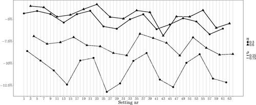
Figure 2. Relative bias in estimating η. The labels on the horizontal axis correspond to the simulation settings as defined in Table 1, the line types distinguish the values of ρ and the symbols denote the value of η. Clear dependence on ρ and on η in the cases with $\rho =0.75.$

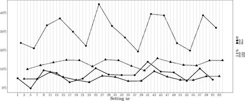
A strong dependence on the autoregressive coefficient ρ is apparent, while ρ itself is always estimated with good accuracy. In particular, higher values of ρ make the estimation of τ₀ and η more difficult. Moreover, when $\rho =0.75$ we can observe a difference in performance attributable to η, namely small η combined with big ρ causes the most biased estimates of the variance of the random intercept and its correlation with the random slope. When $\rho =0.25,$ the relative bias is not large.

Furthermore, we performed a bootstrap analysis on the first simulation setting. We chose a bootstrap sample of B = 350 as this is shown to provide stability in the estimates on the case study (see Supplemental material). In Table 6 we report the average estimate, the standard error as obtained analytically by exploiting the asymptotic properties of ML estimates, the standard error as obtained from the bootstrap analysis (average over the simulated datasets for the bootstrap standard deviation) and the coverage probabilities of the bootstrap confidence intervals. We observe that the direct derivation from the Fisher information matrix undervalues the standard error of the estimates, since the same values from the bootstrap analysis are overall larger and lead to coverage probabilities close to the nominal ones. Increasing the number of bootstrap samples can probably still improve the coverage for some of these parameters.

6. Case study

Understanding self-reported sleep quality and how it links with measurable data is currently of much interest in sleep medicine, since it has been proved to connect with mental and physical health problems (Åkerstedt et al. 1994; Augner 2011; Rahe et al. 2015). In particular, many references investigated the relationship between heart rate variability and sleep quality, possibly with other factors, such as working conditions and well-being. Although researchers do not agree on the direction of the influence, it is well agreed on the existence of a strong link between sleep and both autonomic and cardiovascular response (Kageyama et al. 1998; Burton et al. 2010; Michels et al. 2013).

Our goal is to assess the influence of physiological values, and in particular of derived heart rate measures on perceived sleep quality using the data from a study on sleep quality. Most of the studies apply traditional linear mixed models, but the observed values are often highly variable both within- and between-subjects, with outlying observations and outlying participants. We propose an alternative approach based on the tLMM to take into account the heterogeneity observed in the data. We estimate the influence of night-averaged heart rate (HR) quantities on perceived sleep quality (PSQ) fitting the same model we used in the simulations.

6.1. The data

The study design involved 50 healthy volunteers, of which 54% were females, aging from 40 to 65 years old, as this was considered the age category with the most stable routine and sleep rhythm. All the participants were chosen according to well defined exclusion criteria (diagnosed neurological, cardiovascular, psychiatric, pulmonary or endocrinological disorder; sleep disorder; using sleep, antidepressant or cardiovascular medications; consuming drugs or excessive alcohol; being pregnant; shift working; crossing more than two time zones in the last 2 months). The protocol involved two weeks of home monitoring plus two days in a sleep laboratory. During the first phase, participants were asked to wear an unobtrusive device and to fill in morning and evening questionnaires, where information of the preceding night and day were collected respectively. In the sleep laboratory, besides the collection of this information, other physiological measurements were taken. For more details on the study setup, refer to Goelema et al. (2017). Due to unreliability of the physiological measurements on 8 participants, and the missingness of all the baseline variables relative to one participant, we remained with a dataset consisting of 41 participants.

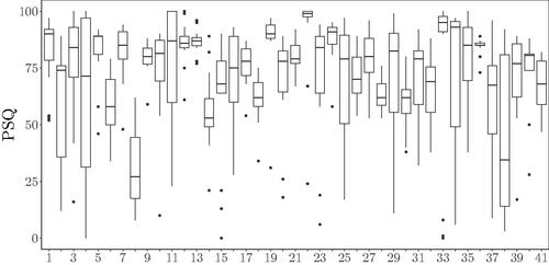
The PSQ, chosen as response variable, was assessed through the morning questionnaire via a visual analog scale ranging from 0 to 100. Being a subjective value, PSQ is highly variable within- and between-participants, with no clear relationship between the level and the variance (see Figure 3). Heterogeneity in this variable was checked via the Levene test (F = 3.05 with df = 40 and $p=6.13e-09$).

Figure 3. PSQ per volunteer. Boxplot of the perceived sleep quality reported by each participant across the whole duration of the study.

The heart beats were extracted from the signal measured by the unobtrusive device and then the average heart rate over 30 s-windows was computed. For the aim of this study, we considered only the aggregated values over nights, namely the night average (HRmean) and the night standard deviation (HRsd) of the 30 s window-averages.

6.2. Preprocessing and data imputation

The data collected during the two nights in laboratory settings were excluded as the change in sleeping conditions might have affected sleep quality, resulting in 14 time points per participant. Furthermore, the rate of missingness in the response variable was 11.13%, while it was 11.74% in HR mean and standard deviation. Since the proposed estimation method requires complete datasets, we performed multiple imputation (R package mice, Zhang 2016) generating 20 complete datasets using some of the baseline and longitudinal variables.

6.3. The fitted model

We fitted a tLMM with random intercept and slope for time as continuous variable and included age, sex, mean HR, standard deviation HR as covariates for the fixed effects, analogous to the one described in Sec. 4.1. We also fitted a linear mixed model with the same fixed and random effects (MIXED procedure of SAS with maximum likelihood estimation, Littell et al. 2007). Note that we used the LMM estimates as starting values for the parameters in the tLMM, together with various initial values for α. Both models were fitted on each imputed dataset separately, and the standard error of the estimates was computed via the bootstrap approach (see Sec. 4.2). Then the final estimates were derived as the mean of the estimates from the analysis of each imputed dataset, and the final standard error of the estimates (combining within- and between-imputed dataset variability) was derived via Rubin’s rule (Rubin 2004). For the LMM we used the MIANALYZE procedure of SAS and for the tLMM we implemented the Rubin’s rule in R. After fitting the model, we sampled 1000 values from the posterior distribution of γ_i (Eq. 23(23) $${\widehat{\gamma }}_i|{\mathbf{Y}}_i\sim \text{Gamma}\left(\frac{\widehat{\alpha }+T_i}{2},\frac{\widehat{\alpha }+{\widehat{\Delta }}_i^2}{2}\right),$$(23) ), and showed their values per subject by means of a boxplot. Analogously to Lin and Lee (2007), we define as outlying the subjects that show extremely small sample values ${\widehat{\gamma }}_i$’s. In fact, a small value of the latent variable indicates that the influence of the corresponding subject (outlier with respect to normality) is downweighted in the estimation of model parameters. To understand better at which level these subjects are outlying (namely in the ${\mathbf{u}}_i$ or in the ${\mathbf{e}}_i$ term), we decomposed the Mahalanobis distance following Eq. (26)(26) $${\widehat{\Delta }}_i^2={\widehat{\Delta }}_{u_i}^2+{\widehat{\Delta }}_{e_i}^2,$$(26) , and checked the value of each component divided by its own expected value under the Gaussian model (Pinheiro, Liu, and Wu 2001).

6.4. Results

After a first analysis of the tLMM, the initially included random slope was left out based on the information criteria (average ${\text{AIC}}_{\text{RIS}}=5142.98$ vs. average ${\text{AIC}}_{\text{RI}}=5138.83$), suggesting that the heterogeneity in the slope was not sufficiently large, and confirmed by the estimate of the variance of the random slope ${\tau }_1=0.000198.$ We thus reduced the model to random intercept only. The estimates for the linear mixed model are shown in Table 7, with the corresponding standard errors between brackets.

Table 6. Results of the bootstrap analysis on the datasets from the first setting.

Parameter	Estimate	Asymptotic er	Bootstrap er	Coverage pr
ζ0	65.00	0.165	0.262	0.935
ζt	1.999	0.037	0.039	0.942
ζa	0.497	0.172	0.183	0.944
ζg	2.506	0.235	0.362	0.955
α	1.699	0.376	0.409	0.980
τ0	0.914	0.145	0.157	0.885
τ1	0.243	0.030	0.031	0.918
η	0.337	0.174	0.192	0.920
${\sigma }^2$	0.771	0.091	0.112	0.954
ρ	0.247	0.045	0.047	0.955

Results of the bootstrap analysis with 350 samples from each of the 1000 simulated datasets from setting 1. The asymptotic error is the one obtained via the Fisher information matrix and is compared to the one obtained via the bootstrap method. In the last column is shown the coverage probability as obtained with the bootstrap standard deviation.

As for the LMM, also for the tLMM the random slope did not improve the fit and thus in Table 8 we report the estimates of the model with random intercept only, with their standard deviations obtained via the bootstrap approach. The results shown in the table correspond to the starting value ${\alpha }_0=1.5.$

Table 7. Coefficients of the LMM.

Fixed Effects
ζ0	ζg	ζa	ζHRm	ζHRs	ζt
86.69 (18.24)	5.86 (3.86)	−0.21 (0.30)	−0.22 (0.18)	0.52 (0.75)	0.61 (0.23)
Variance–covariance components
${\tilde{\tau }}_0^2$	${\tilde{\sigma }}_0^2$	ρ
114.08 (32.69)	444.31 (29.65)	−0.06 (0.05)

Estimates of the coefficients of the LMM and corresponding standard error between brackets. Fitted with the MIXED procedure in SAS software choosing the maximum likelihood estimation method. The estimates and standard errors are pooled with the procedure MIANALYZE. Some parameters have a tilde in the notation as they cannot be directly compared with the corresponding parameter in the tLMM Pinheiro, Liu, and Wu (2001).

The average perceived sleep quality corrected by the mentioned factors is 84.84 ± 6.63, and is negatively affected by an increased mean heart rate over the night (${\zeta }_{\mathit{HRm}}=-0.18\pm 0.16$), while it is on average higher for females (${\zeta }_g=6.93\pm 4.41$). At the same time, differences in age seem to play no role in the perception of a good night sleep, as well as the fixed effect of the night standard deviation of the heart rate. There is a positive effect of time and a significant difference between participants in overall mean. The residuals have a variance of ${\sigma }^2=440.55\pm 13.28,$ with no significant autoregressive structure. Note that both parameters of the gamma distribution are equal to $\alpha =\beta =1.51\pm 0.85,$ which justifies the choice of tLMM over traditional LMMs, and this is confirmed by the information criteria (average ${\text{AIC}}_{t\text{LMM}}=5138.83$ against average ${\text{AIC}}_{\text{LMM}}=5210.18$). Furthermore, while the estimates do not show extreme differences, the tLMM significantly reduces the standard deviation compared to the LMM. This might be explained by the fact that the heterogeneity affects more the confidence with which we can estimate the parameters than the estimates themselves, and is another observation in favor of the t model over the traditional one.

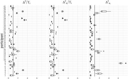
Finally, we used the tLMM fit to identify outlying participants with respect to normality (as discussed in Sec. 4.3), and applied the rule suggested by Lin and Lee (2007). Values ${\widehat{\gamma }}_i$’s substantially lower than 1 indicate a possibly outlying subject. In Figure 4 we show the values sampled from the posterior distribution for each participant via a boxplot. In total each boxplot refers to 1000 values sampled from each of the 20 posterior distributions (20 imputed datasets and relative estimated parameters). We chose to pool the values across imputations because there was no large deviation across imputations. Looking at the plot, we conclude that participants 2, 3, 4, 11, 15, 16, 25, 29, 33, 34, 37 and 38 should be regarded as potential outliers for the LMM fit. It is also interesting to understand at which level the participants are outlying, because even in case their overall behavior is in line with the sample, they may still have outlying behavior at the level of random effects or residuals separately. Following the method of Pinheiro, Liu, and Wu (2001), we plotted the values of the two components of the Mahalanobis distance and the distance itself divided by their own expected value under normality. Cases in which these values are larger than one can be regarded as outliers. In Figure 5 we show these values corresponding to the 20 imputations in our case study: each boxplot collects the values of one of these quantities across the 20 imputed datasets for one single participant. The three plots are for ${\Delta }^2/T_i,$ ${\Delta }_{e_i}^2/T_i$ and ${\Delta }_{u_i}^2$ respectively. We can observe that participants 2, 4, 8, 14, 15, 22, 37, 38 are outlying at the ${\mathbf{u}}_i$ level, while subjects 2, 3, 4, 11, 15, 16, 25, 29, 33, 34, 37, 38 are outlying at the ${\mathbf{e}}_i$ level. It is worth noticing that participants 8, 14 and 22 are flagged as potential outliers when looking at the components of the Mahalanobis distance, while they would not be detected when looking at the total residuals or at the posterior conditional distribution of the γ_i’s. The analysis of outlying observations clearly demonstrates the potential of the tLMM over the more common LMM approach.

Figure 4. γ_i. Boxplot of 1000 sampled γ_i values per participant. The horizontal line at value 1 separates the bulk of observations from the outlying participants boxplots that are significantly below 1 indicate outlying participants.

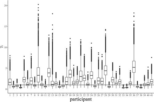
Figure 5. Decomposition of the Mahalanobis distance. (a) ${\widehat{\Delta }}_i^2/T_i$ (b) ${\widehat{\Delta }}_{e_i}^2/T_i$ (c) ${\widehat{\Delta }}_{u_i}^2.$

7. Discussion

In this paper, we presented a thorough analysis of the tLMM, with particular focus on model definition and parameter estimation. For the first part, we provided the mathematical formulation of non-identifiability for tLMMs and gave explanation to the common choice of equal parameters of the gamma distribution, normally not justified. It is worth noticing how different gamma distributions actually end up in the same marginal distribution of the response variable ${\mathbf{Y}}_i.$ Thus, the same t can have different interpretations.

Identifiability issues that arise in the variance-covariance structure are theoretically shown by comparing the covariance matrix corresponding to two different sets of parameters, illustrating the procedure under some popular assumptions on the variance-covariance structure of random effects and residuals. The effect of unidentifiability on estimation is illustrated via a small simulation study. As expected, the estimates of the fixed effects are still reliable, their standard deviation is slightly higher, but this might be due to the lower number of settings compared with the identifiable case. The main effect of unidentifiability is reflected in the estimation of the variance-covariance parameters, and this is crucial when using the t mixed model for the analysis of variances (Chinchilli, Esinhart, and Miller 1995; Lin, Raz, and Harlow 1997; Welsh and Richardson 1997). Since the method convergences also in this case, identifiability issues are difficult to spot a posteriori and should be checked in the phase of model definition and formulation.

Then we investigated the reliability of an existing estimation method in case the model is identifiable. We extended the direct maximum likelihood approach of Lin and Lee (2006) to allow for two correlated random effects and an autoregressive correlation structure of first order. The method is direct, easy to understand, reasonably fast and fully reproducible.

We assessed its performance via an intensive simulation study under the traditional choice of $\alpha =\beta ,$ and showed that the fixed effects can be accurately estimated in all the considered settings, also with a relatively small amount of subjects and a large number of repeats. This analysis is quite unique, as previous work on the robustness of estimation methods is limited, and even when it exists, it simulates a small number of observations (Pinheiro, Liu, and Wu 2001) or a relatively simple correlation structure (Lin, Raz, and Harlow 1997). This is the component that is most difficult to estimate. In fact, we concluded that for some sets of true values the estimation of the variance-covariance parameters is less stable, in particular for η and τ₀ when the coefficient of autocorrelation ρ is large. This problem is normally overcome in the literature by employing Bayesian approaches (Lin and Lee 2007) or expectation-maximization algorithms (Lin 2008), or by avoiding the coupling of both random intercept and slope with autoregressive correlation structures. For example Lin and Lee (2006) explore random intercept with autoregressive correlation, but simplify the correlation structure when including also a random intercept. The choice might be due to their case study, concerning 17 observations on a maximum of 18 participants, which might be very critical for the estimation accuracy. In fact, we showed that thanks to the optimal properties of ML estimation the accuracy can be improved by increasing the number of subjects in the study, which is commonly even larger in panel studies than it was in our simulation study. Furthermore, our study demonstrates that relying on the asymptotic properties of the ML estimates in this case can lead to underestimation of the actual variability in the estimates. Therefore we proposed a bootstrap approach to estimate the standard error of the estimates.

The analysis of sleep data led to conclusions that slightly differ from the literature (Kageyama et al. 1998; Michels et al. 2013). This might be due to the HR variables that were taken into account, aggregated at night level, or to the novel approach accounting for additional heterogeneity. In fact, even choosing higher starting values for the parameters of the gamma distribution (e.g. ${\alpha }_0=10$), led to the same estimate of the hyper-parameter, supporting the choice of a model with underlying heavy-tailed distribution. The choice between these assumptions will require further investigation.

Note that the speed and rate of convergence of the estimation method could be increased by choosing an alternative optimization procedure and by providing the gradient of the likelihood function. Furthermore, more research is needed to overcome the limitation of the current method in handling missing values. Also the model could be extended by empowering different heterogeneity factors for the random effects and for the residuals, as already highlighted by Pinheiro, Liu, and Wu (2001). Another extension would involve replacing the gamma distribution with more general exponential probability distributions, and relaxing the hypothesis of conditional independence between random effects and residuals. Finally, future research should focus on deriving specific measures to assess the goodness of fit of the t distribution.

Acknowledgments

This research was performed within the framework of the strategic joint research program on Data Science between TU/e and Philips Electronics Nederland B.V. We thank the anonymous reviewers for carefully reading our manuscript and providing insightful feedback and suggestions, as this resulted in a significant improvement of the manuscript.

Data availability statement

The data that support the findings of this study are available from Philips Research. Restrictions apply to the availability of these data, which were used under license for this study. The codes are available from the corresponding author on request.

Disclosure statement

No potential conflict of interest was reported by the authors.

Table 8. Coefficients of the tLMM.

Fixed effects
ζ0	ζg	ζa	ζHRm	ζHRs	ζt
84.84 (6.63)	6.93 (4.41)	−0.12 (0.24)	−0.18 (0.16)	0.24 (0.54)	0.45 (0.20)
Variance–covariance components
τ0	${\sigma }^2$	Ρ	Α
12.75 (2.55)	440.55 (13.28)	−0.01 (0.07)	1.51 (0.85)

Estimates of the coefficients of the tLMM and corresponding standard deviations in the brackets. Fitted with the direct ML procedure described in Sec. 4, starting values the LMM estimates in Table 7 and ${\alpha }_0=1.5.$

References

- Åkerstedt, T., K. Hume, D. Minors, and J. Waterhouse. 1994. The meaning of good sleep: A longitudinal study of polysomnography and subjective sleep quality. Journal of Sleep Research 3 (3):152–8.
- Augner, C. 2011. Associations of subjective sleep quality with depression score, anxiety, physical symptoms and sleep onset latency in students. Central European Journal of Public Health 19 (2):115. doi:https://doi.org/10.21101/cejph.a3647.
- Burton, A., K. Rahman, Y. Kadota, A. Lloyd, and U. Vollmer-Conna. 2010. Reduced heart rate variability predicts poor sleep quality in a case–control study of chronic fatigue syndrome. Experimental Brain Research 204 (1):71–8. doi:https://doi.org/10.1007/s00221-010-2296-1.
- Chinchilli, V. M., J. D. Esinhart, and W. G. Miller. 1995. Partial likelihood analysis of within-unit variances in repeated measurement experiments. Biometrics 51 (1):205–16. doi:https://doi.org/10.2307/2533326.
- Efron, B., and R. J. Tibshirani. 1994. An introduction to the bootstrap. Boca Raton, Florida: CRC Press.
- Goelema, M. S., M. Regis, R. Haakma, E. R. Van Den Heuvel, P. Markopoulos, and S. Overeem. 2017. Determinants of perceived sleep quality in normal sleepers. Behavioral Sleep Medicine 17 (4):388–97. doi:https://doi.org/10.1080/15402002.2017.1376205.
- Ho, H. J., and T.-I. Lin. 2010. Robust linear mixed models using the skew t distribution with application to schizophrenia data. Biometrical Journal 52 (4):449–69. doi:https://doi.org/10.1002/bimj.200900184.
- Janzén, D. L. I., M. Jirstrand, M. J. Chappell, and N. D. Evans. 2019. Three novel approaches to structural identifiability analysis in mixed-effects models. Computer Methods and Programs in Biomedicine 171:141–52. doi:https://doi.org/10.1016/j.cmpb.2016.04.024.
- Johnson, S. G. 2014. The nlopt nonlinear-optimization package.
- Kageyama, T., N. Nishikido, T. Kobayashi, Y. Kurokawa, T. Kaneko, and M. Kabuto. 1998. Self-reported sleep quality, job stress, and daytime autonomic activities assessed in terms of short-term heart rate variability among male white-collar workers. Industrial Health 36 (3):263–72. doi:https://doi.org/10.2486/indhealth.36.263.
- Kotz, S., and S. Nadarajah. 2004. Multivariate t-distributions and their applications. Cambridge, England: Cambridge University Press.
- Laird, N. M., and J. H. Ware. 1982. Random-effects models for longitudinal data. Biometrics 38 (4):963–74. doi:https://doi.org/10.2307/2529876.
- Lange, K. L., R. J. Little, and J. M. Taylor. 1989. Robust statistical modeling using the t distribution. Journal of the American Statistical Association 84 (408):881–96. doi:https://doi.org/10.2307/2290063.
- Lavielle, M., and L. Aarons. 2016. What do we mean by identifiability in mixed effects models? Journal of Pharmacokinetics and Pharmacodynamics 43 (1):111–22. doi:https://doi.org/10.1007/s10928-015-9459-4.
- Lin, T.-I. 2008. Longitudinal data analysis using t linear mixed models with autoregressive dependence structures. Journal of Data Science 6:333–55.
- Lin, T. I., and J. C. Lee. 2006. A robust approach to t linear mixed models applied to multiple sclerosis data. Statistics in Medicine 25 (8):1397–412. doi:https://doi.org/10.1002/sim.2384.
- Lin, T. I., and J. C. Lee. 2007. Bayesian analysis of hierarchical linear mixed modeling using the multivariate t distribution. Journal of Statistical Planning and Inference 137 (2):484–95. doi:https://doi.org/10.1016/j.jspi.2005.12.010.
- Lin, T.-I., and W.-L. Wang. 2019. Multivariate-t linear mixed models with censored responses, intermittent missing values and heavy tails. Statistical Methods in Medical Research 0:1–17. doi:https://doi.org/10.1177/0962280219857103.
- Lin, X., J. Raz, and S. D. Harlow. 1997. Linear mixed models with heterogeneous within-cluster variances. Biometrics 53 (3):910–23. doi:https://doi.org/10.2307/2533552.
- Littell, R. C., G. A. Milliken, W. W. Stroup, R. D. Wolfinger, and O. Schabenberger. 2007. SAS for mixed models. Cary, North Carolina: SAS Institute.
- Matos, L. A., M. O. Prates, M.-H. Chen, and V. H. Lachos. 2013. Likelihood-based inference for mixed-effects models with censored response using the multivariate-t distribution. Statistica Sinica 23 (3):1323–45. doi:https://doi.org/10.5705/ss.2012.043.
- Michels, N., E. Clays, M. D. Buyzere, B. Vanaelst, S. D. Henauw, and I. Sioen. 2013. Children's sleep and autonomic function: low sleep quality has an impact on heart rate variability. Sleep 36 (12):1939–46. doi:https://doi.org/10.5665/sleep.3234.
- Pinheiro, J. C., C. Liu, and Y. N. Wu. 2001. Efficient algorithms for robust estimation in linear mixed-effects models using the multivariate t distribution. Journal of Computational and Graphical Statistics 10 (2):249–76. doi:https://doi.org/10.1198/10618600152628059.
- Powell, M. J. 2008. Developments of NEWUOA for minimization without derivatives. IMA Journal of Numerical Analysis 28 (4):649. doi:https://doi.org/10.1093/imanum/drm047.
- R Core Team. 2016. R: A language and environment for statistical computing. Vienna, Austria: R Foundation for Statistical Computing.
- Rahe, C., M. E. Czira, H. Teismann, and K. Berger. 2015. Associations between poor sleep quality and different measures of obesity. Sleep Medicine 16 (10):1225–8. doi:https://doi.org/10.1016/j.sleep.2015.05.023.
- Rubin, D. B. 2004. Multiple imputation for nonresponse in surveys, vol. 81. Hoboken, New Jersey: John Wiley & Sons.
- Samani, E. B. 2014. Sensitivity analysis for the identifiability with application to latent random effect model for the mixed data. Journal of Applied Statistics 41 (12):2761–76. doi:https://doi.org/10.1080/02664763.2014.929641.
- Upton, G., and I. Cook. 2014. A dictionary of statistics 3e. Oxford, UK: Oxford University Press.
- Van der Vaart, A. W. 1998. Asymptotic statistics, vol. 3. Cambridge, England: Cambridge University Press.
- Wang, W.-L. 2013. Multivariate t linear mixed models for irregularly observed multiple repeated measures with missing outcomes. Biometrical Journal 55 (4):554–71. doi:https://doi.org/10.1002/bimj.201200001.
- Wang, W.-L. 2019. Mixture of multivariate t nonlinear mixed models for multiple longitudinal data with heterogeneity and missing values. TEST 28 (1):196–222. doi:https://doi.org/10.1007/s11749-018-0612-4.
- Wang, W.-L., and T.-H. Fan. 2011. Estimation in multivariate t linear mixed models for multiple longitudinal data. Statistica Sinica 21 (4):1857–80. doi:https://doi.org/10.5705/ss.2009.306.
- Wang, W.-L., and T.-H. Fan. 2012. Bayesian analysis of multivariate t linear mixed models using a combination of IBF and Gibbs samplers. Journal of Multivariate Analysis 105 (1):300–10. doi:https://doi.org/10.1016/j.jmva.2011.10.006.
- Wang, W.-L., and T.-I. Lin. 2014. Multivariate t nonlinear mixed-effects models for multi-outcome longitudinal data with missing values. Statistics in Medicine 33 (17):3029–46. doi:https://doi.org/10.1002/sim.6144.
- Wang, W.-L., and T.-I. Lin. 2015. Bayesian analysis of multivariate t linear mixed models with missing responses at random. Journal of Statistical Computation and Simulation 85 (17):3594–612. doi:https://doi.org/10.1080/00949655.2014.989852.
- Wang, W.-L., T.-I. Lin, and V. H. Lachos. 2018. Extending multivariate-t linear mixed models for multiple longitudinal data with censored responses and heavy tails. Statistical Methods in Medical Research 27 (1):48–64. doi:https://doi.org/10.1177/0962280215620229.
- Wang, W. 2013. Identifiability of linear mixed effects models. Electronic Journal of Statistics 7 (0):244–63. doi:https://doi.org/10.1214/13-EJS770.
- Wang, W. 2017. Checking identifiability of covariance parameters in linear mixed effects models. Journal of Applied Statistics 44 (11):1938–46. doi:https://doi.org/10.1080/02664763.2016.1238050.
- Welsh, A., and A. Richardson. 1997. Approaches to the robust estimation of mixed models. Handbook of Statistics 15:343–84.
- Wolfram Research, Inc. 2019. Mathematica, version 12.0. Champaign, IL: Wolfram Research, Inc.
- Ypma, J. Introduction to nloptr: An R interface to NLopt. Technical report, Technical report. 2014.
- Zhang, Z. 2016. Multiple imputation with multivariate imputation by chained equation (MICE) package. Annals of Translational Medicine 4 (2):30. doi:https://doi.org/10.3978/j.issn.2305-5839.2015.12.63.