Discrimination with unidimensional and multidimensional item response theory models for educational data

Abstract

Achievement tests are used to characterize the proficiency of higher-education students. Item response theory (IRT) models are applied to these tests to estimate the ability of students (as latent variable in the model). In order for quality IRT parameters to be estimated, especially ability parameters, it is important that the appropriate number of dimensions is identified. Through a case study, based on a statistics exam for students in higher education, we show how dimensions and other model parameters can be chosen in a real situation. Our model choice is based both on empirical and on background knowledge of the test. We show that dimensionality influences the estimates of the item-parameters, especially the discrimination parameter which provides information about the quality of the item. We perform a simulation study to generalize our conclusions. Both the simulation study and the case study show that multidimensional models have the advantage to better discriminate between examinees. We conclude from the simulation study that it is safer to use a multidimensional model compared to a unidimensional if it is unknown which model is the correct one.

Keywords:

• Achievement tests
• Discrimination
• Multidimensional four parameter logistic model
• Multidimensional graded response model
• Multidimensional item response theory

1. Introduction

In different disciplines of studies like statistics, education, psychology, to mention a few, tests might be multidimensional. This means that these tests measure two or more dimensions of ability, also called constructs. The tests consist of several questions, called items. To model such items, a multidimensional item response theory (MIRT) is a widely used tool. The MIRT models are appropriate since these models explain the relationship between two or more latent (unobserved) variables and the probability to correctly answer the particular question by the examinee. The MIRT model has become a popular tool for the analysis of test content, computerized adaptive testing and equating of test calibrations noticed by Reckase (2007).

Generally, MIRT models can be categorized into compensatory and non-compensatory models. More often than not, MIRT models are compensatory allowing the dimensions to interact. As Yang (2007) points out, the literature of educational research is dominated by compensatory model applications (Reckase 1979; Drasgow and Parsons 1983; Yen 1984; Way, Ansley, and Forsyth 1988; Reckase and McKinley 1991; Kirisci, Hsu, and Yu 2001). Our focus remains on compensatory models for this article. For a compensatory model, the high ability, in terms of probability to correctly answer the question in one dimension can compensate for the low ability in another dimension. On the other hand, a non-compensatory model does not permit this. Therefore, one needs to be proficient in each ability to obtain the highest score.

In MIRT models the emphasis has not been to minimize the number of dimensions as is the case in factor analysis. Reckase (1997) analyzed item response data even with 25 or more dimensions. However, most of the recent applications of MIRT have used fewer dimensions either due to the limitations in estimation programs or because it is useful, on other hand, to plot the results but it is difficult to plot more than three dimensions. The usage of unidimensional item response theory (UIRT) models is not new to the disciplines of education and psychology. However, meeting the unidimensionality assumption for ability is difficult in some achievement tests (Reckase 1985; Hambleton, Swaminathan, and Rogers 1991).

Many researchers (Spencer 2004; De La Torre and Patz 2005; Yang 2007; Kose and Demirtasli 2012) have compared unidimensional and multidimensional models. They have demonstrated that the ability and item parameters have less estimation error and provide more precise measurements under MIRT due to the fact that the number of latent traits underlying item performance increase. Moreover, the model-data fit indexes are in the favor of MIRT models. Wiberg (2012) used multidimensional college admission test data to examine the consequences of applying the UIRT models. She discovered from a simulation study that MIRT gives better model fit result compared to UIRT. However, the result of a consecutive UIRT approach is proximate to MIRT. She concluded that if the test had between-item multidimensionality, the use of consecutive UIRT instead of MIRT models is not harmful and it may be easier to interpret logically.

Hooker, Finkelman, and Schwartzman (2009) have highlighted a paradox occuring with MIRT in contrast to UIRT: if the answer of an examinee to an item is changed from correct to wrong, it could happen that the estimated ability decreases in some dimension. Further insights to this potential issue have been given by Finkelman, Hooker, and Wang (2010), Hooker (2010), and Jordan and Spiess (2012, 2018). The mentioned references argue for the need to address this issue to avoid unfairness in the test. Other researchers have contrasting views. According to van Rijn and Rijmen (2012), preventing paradoxical results are less relevant as long as one has not a contest perspective on a test. According to van der Linden (2012), the convergence of ability estimates (e.g., the MLE) to the true ability is of main importance; additional information improves estimates even if paradoxical results occur (Reckase and Luo 2015). In contrast to this view, Jordan and Spiess (2012) point out that the concept of fairness is an individual concept and refers not to infinite fictitious repetitions like quality of estimates.

The discrimination parameter of the model is a measure of the differential capability of an item. An item is considered valuable if it well discriminates subjects with ability levels in a range of interest for the exam. A larger value of the discrimination parameter demonstrates that the probability to correctly answer a question rapidly increases with the increase in the ability. The high value of discrimination parameter yields a steeper slope of the item characteristic curve (ICC), and the item has then a better possibility to differentiate subjects around the difficulty level of the item. Items with higher discrimination power can therefore contribute more in assessment precision in comparison to items with a low discrimination power, provided that the item-difficulty is in the scope of the exam. So, a feature which is of importance for educationalists is the capability of an item to discriminate between examinees. In UIRT model, items can discriminate subjects on one direction, whereas items in MIRT model differentiate examinees on each dimension.

The objectives of this study are: (1) to show how the question of dimensionality can be explored for an achievement test in higher education, (2) to show how a good model for analysis can be chosen in a real situation and (3) to investigate the impact of the number of dimensions in the chosen model on the discrimination parameter’s estimate.

2. Data of case study

Data used in this paper are acquired from a statistics exam for higher education students. This exam was taken by 238 examinees in March 2015. There were in total 16 questions in this exam which had a mixed-format consisting of 15 multiple-choice items and one free-response item. The first 15 questions Q₁ to Q₁₅ offer 5 options and one of them is correct. The responses have been dichotomized with the values 0 (wrong answer) and 1 (correct answer). The last question Q₁₆ offers a maximum of 10 points. We have polychotomized response of this item with the values 0, 1, 2, 3, 4 and 5. The codification 0 represents if the student got 0 points and 1 for $0<\text{points}\le 2$ and 2 for $2<\text{points}\le 4$ in the question, and so on. The characteristics of the exam and the percentage of correct answers are summarized in Table 1. Question 1 was easiest and question 12 toughest in the exam for the students according to this percentage. Most of the students were able to get 10 points for the last question. The item questions target different areas of statistics according to the teacher’s intentions, e.g., basic statistics, testing of hypothesis, regression, see Table 1.

Table 1. Data description.

Question	Area	Percentage correct
Q1	Basic statistics	93.3
Q2	Basic statistics	92.9
Q3	Basic statistics	54.6
Q4	Basic statistics (graphical)	79.8
Q5	Contingency table	96.6
Q6	Contingency table	60.5
Q7	Contingency table	75.2
Q8	Binomial distribution	79.0
Q9	Normal distribution	77.3
Q10	Normal distribution	60.1
Q11	Testing of hypothesis	52.5
Q12	Testing of hypothesis	42.4
Q13	Testing of hypothesis	87.0
Q14	Regression	75.6
Q15	Regression	87.0
Question	Area	Percentage in each category
		0	1	2	3	4	5
Q16	Chi-square test	9.7	2.5	3.4	5.0	27.7	51.7

3. Materials and methods

3.1. Unidimensional item response theory models (UIRT)

Let U_ij be the dichotomous response of examinee j $(j=1,2,\dots ,N)$ to item i $(i=1,2,\dots ,n)$ and $P(U_{ij}=1|{\theta }_j;a_i,b_i,c_i,g_i)$ the probability of a correct response by examinee j to item i with ability ${\theta }_j.$ Commonly used IRT models for dichotomous responses are two- and three-parameter logistic models. However, the four-parameter logistic (4PL) model recently received more attention and some researchers highlighted its potential for practical purposes and from a methodological point of view (Magis 2013). The R package catR recently introduced the 4PL model as a baseline IRT model for computerized adaptive test (CAT) generation (Magis and Raîche 2012). The 4PL model can be expressed as (1) $$P\left(U_{ij}=1|{\theta }_j;a_i,b_i,c_i,g_i\right)=c_i+\frac{g_i-c_i}{1+e^{-a_i({\theta }_j-b_i))}}$$(1) where ${\theta }_j$ is the ability of examinee j, $b_i$ is the difficulty of item i (location of the item response function), $a_i>0$ is the discrimination of item i that determines the steepness of the item response function, $c_i$ is the lower asymptotic parameter for the $i^{th}$ item response function, $g_i$ is the upper asymptotic parameter for the $i^{th}$ item response function.

The three-parameter logistic (3PL) model is a special case of the 4PL model with $g_i=1.$ The two-parameter logistic (2PL) model is a special case with $g_i=1$ and $c_j=0.$

For the polychotomized free-response item we have used the graded-response (GR) model which was first introduced by Samejima (1969) for ordered categorical responses. This model is a generalization of the 2PL model. The probability of the $j$ th examinee to respond the $k$ th out of $r_i$ categories for the $i$ th item is expressed as (2) $$\begin{array}{c}{P}_{\mathit{ijk}}=P\left(U_{ij}=k|{\theta }_j;a_i,b_i\right)=P\left(U_{ij}\ge k|{\theta }_j;a_i,b_i\right)-P\left(U_{ij}\ge k+1|{\theta }_j;a_i,b_i\right),\\ P\left(U_{ij}\ge k|{\theta }_j;a_i,b_i\right)=\frac{1}{1+e^{-a_i({\theta }_j-b_{ik})}}, k=1,2,\dots ,r_i-1,\\ P\left(U_{ij}\ge 0|{\theta }_j;a_i,b_i\right)=1,\\ P\left(U_{ij}\ge r_i|{\theta }_j;a_i,b_i\right)=0,\end{array}$$(2) where $a_i$ and ${\theta }_j$ are again discrimination and ability parameter, respectively, and $b_i=(b_{i1},\dots ,b_{i(r_i-1)})$ is a vector of category intercepts for item i.

3.2. Multidimensional item response theory models (MIRT)

In MIRT models, the probability of success is modeled as a function of multiple ability dimensions. Each person has a vector ${\theta }_j=({\theta }_{j1},\dots ,{\theta }_{jm})$ of ability parameter values. Each item has vector of discrimination parameter values $a_{il}=(a_{i1},\dots ,a_{im}),$ one difficulty parameter $d_i=-a_i{b}_i,$ a guessing $c_i$ and an upper asymptote parameter $g_i$ (Reckase 2009). We can write a four-parameter logistic MIRT model (M4PL) as generalization of the UIRT model (1)(1) $$P\left(U_{ij}=1|{\theta }_j;a_i,b_i,c_i,g_i\right)=c_i+\frac{g_i-c_i}{1+e^{-a_i({\theta }_j-b_i))}}$$(1) by replacing $a_i{\theta }_j$ with ${\sum }_{l=1}^m{a}_{il}{\theta }_{jl}$ where m is the total number of dimensions. The M3PL (or M2PL) is again a special case of the M4PL model by setting $g_i=1$ (or $g_i=1$ and $c_i=0$). The multidimensional graded response (MGR) model generalizes formula (2)(2) $$\begin{array}{c}{P}_{\mathit{ijk}}=P\left(U_{ij}=k|{\theta }_j;a_i,b_i\right)=P\left(U_{ij}\ge k|{\theta }_j;a_i,b_i\right)-P\left(U_{ij}\ge k+1|{\theta }_j;a_i,b_i\right),\\ P\left(U_{ij}\ge k|{\theta }_j;a_i,b_i\right)=\frac{1}{1+e^{-a_i({\theta }_j-b_{ik})}}, k=1,2,\dots ,r_i-1,\\ P\left(U_{ij}\ge 0|{\theta }_j;a_i,b_i\right)=1,\\ P\left(U_{ij}\ge r_i|{\theta }_j;a_i,b_i\right)=0,\end{array}$$(2) by replacing $a_i{\theta }_j$ with ${\sum }_{l=1}^m{a}_{il}{\theta }_{jl}$ using the vector of category intercepts $d_i=(d_{i1},\dots ,d_{i(r_i-1)})$ for item i, where $d_{ik}=-a_i{b}_{ik}.$

3.3. Exploratory and confirmatory MIRT models

The MIRT models are either exploratory or confirmatory depending upon the available information at the model specification step. An exploratory MIRT model is useful to explore the possible structure of a set of test items without preconceived structure on the items, or even when unconstrained solution is seen as a strong test to verify the hypothesized structure of test items. After applying exploratory MIRT model one could identify underlying structure of a set of test items. The confirmatory MIRT models are useful when we have clear hypothesis about structure of set of items in an examination taken by students. In fact, the confirmatory MIRT model needs to have a specified number of latent abilities to explain the pattern of relationships between the items. In confirmatory MIRT the researcher postulates the relationship between items and specific number of latent variables a priori, based on knowledge of the theory, empirical research, or both. This hypothesized structure is statistically tested by the researcher. The confirmatory MIRT models are valuable to measure aspects such as different knowledge structure of examinees, multiple abilities, strategies, satisfaction level and attitudes on which persons differ quantitatively.

It is common that in exploratory analyses a model is used where all ability parameters can influence all items (Figure 1, middle) called within-item multidimensionality. A typical confirmatory analysis uses models where the different abilities influence disjoint sets of items (Figure 1, right) denoted as between-item multidimensionality, see Adams, Wilson, and Wang (1997) and Hartig and Höhler (2009). We use a model with between-item multidimensionality later for an exploratory analysis of our case study. The MIRT model with between-item multidimensionality has also been called MIRT model of simple structure or multiunidimensional IRT model; Sheng and Wikle (2007) compare this model with the UIRT model. It has been noted e.g., by Jordan and Spiess (2012) that the model with between-item multidimensionality and with ML estimation avoids the issue of paradoxical results mentioned in the introduction (however, if a Bayesian analysis is used and the dimension is at least 3, paradoxical results still are possible, see Finkelman, Hooker, and Wang (2010)).

Figure 1. The graphical representation of a unidimensional and a multidimensional model with within-item and with between-item multidimensionality. The left panel represents the univariate model. The middle panel depicts a multidimensional model with within-item multidimensionality, and the right panel indicates a multidimensional model with between-item multidimensionality.

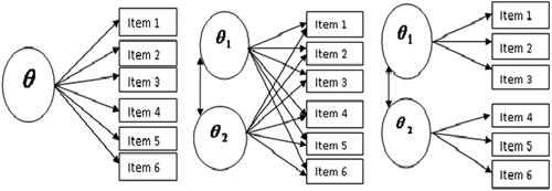
A variant of a MIRT model with between-item multidimensionality is the consecutive UIRT model where the items belonging to one ability are analyzed as separate models. In the right panel of Figure 1, we remove the arrow between θ₁ and θ₂ to illustrate the consecutive UIRT.

3.4. The ability parameters in the models

The ability of the examinees is characterized by a single ability parameter ${\theta }_j$ in the UIRT or by a multidimensional parameter vector ${\theta }_j={({\theta }_{j1},\dots ,{\theta }_{jm})}^T$ in the MIRT. We assume that the investigated population has normally distributed ability parameters with standardized variance 1, i.e., $${\theta }_j\sim N(0,1) \text{or} {\theta }_j\sim N(0,C)$$ with covariance matrix C having a diagonal of 1’s, see (Reckase 2007; Chalmers 2012) and specifically for m = 1, (Baker and Kim 2004; Rizopoulos 2006). The standardization is important to make the discrimination parameters $a_i$ in the model well-defined (identifiable) as otherwise dividing all abilities by a factor and multiplying all discrimination parameters by the same factor would lead to the same data fit. We think that this is even more important from an interpretation perspective than from a theoretical perspective: it is beneficial to make discrimination parameters comparable across different analysis models as well as across different examinations.

3.5. Model estimation

First, it is useful to define the response data in the form of an indicator function $$\chi (u_{ij},k)=\{\begin{array}{cc}1,\hfill & \text{if} u_{ij}=k,\hfill \\ 0,\hfill & \text{otherwise}.\hfill \end{array}$$ Let ψ be the set of all unknown item parameters. The conditional likelihood for the j_th $N\times 1$ response pattern vector, $U_j$ can be defined as $$L(u_j|\psi ,\theta )=\prod _{i=1}^n\prod _{k=0}^{r_i-1}p{(U_{ij}=k|\psi ,{\theta }_j)}^{\chi (U_{ij},k)},$$ where the number of categories r_i is set to 2 for dichotomous items ($k\in \{0,1\}$). Denoting the density of the ability parameter by $g(\theta )$ (recall that we assume them having a standardized multivariate normal distribution), we integrate them out of the likelihood function. This yields to the marginal likelihood equation of the observed data U (N × n data matrix) $$L(\psi |U)=\prod _{j=1}^N\left[{\int }_{-\infty }^{\infty }\dots {\int }_{-\infty }^{\infty }L(u_j|\psi ,\theta )g(\theta )d(\theta )\right].$$ For estimation of the IRT models, the recommended method in case of a small number of dimensions (less than 4) is the expectation maximization (EM) algorithm by using fixed Gauss-Hermite quadrature while the Metropolis-Hastings Robbins-Monro (MH-RM) algorithm and Quasi-Monte Carlo EM (QMCEM) estimation are recommended in case of higher dimensionality or when multidimensional confirmatory model is required (Chalmers 2012). For higher dimension, the EM algorithm solution becomes difficult as we require large number of numerical quadrature in the E-step to evaluate high-dimensional integrals in the likelihood function of the item parameters.

3.6. Models comparison criteria

To evaluate the goodness of fit of different competing models, we have used following statistical approaches: Akaike information criterion (AIC), bias corrected AIC (AICc), Bayesian information criterion (BIC) and sample size adjusted BIC (SABIC). These statistics are based on the log-likelihood of a fitted model, sample size and number of parameters estimated as follows: $\mathit{AIC}=-2LL+2p,\mathit{AICc}=-2LL+2p+\frac{2p(p+1)}{N-p-1},$ $\mathit{BIC}=-2LL+\hspace{0.17em}\text{log}\hspace{0.17em}(N)p,\mathit{SABIC}=-2LL+\hspace{0.17em}\text{log}\hspace{0.17em}\left(\frac{N+2}{24}\right)p.$ Here p is the number of item parameters being estimated (= number of item parameters $-\frac{m(m-1)}{2}$), LL is the log likelihood of the model, N indicates the number of examinees and m represents number of dimensions. Smaller AIC, AICc, BIC and SABIC values indicate better fit. Like BIC, SABIC places a penalty based on sample size for adding parameters, but the penalty is not as high as for BIC. We note that we use here the above mentioned form of AICc since it is the version implemented in the R package mirt which we use for analysis and since Burnham and Anderson (2002) suggested that this form could be used generally. However, AICc in general is model dependent, see Section 7.4 of Burnham and Anderson (2002).

The likelihood ratio tests were also conducted between the nested models to find out whether a more complicated model fits better than the simple one.

3.7. Determination of number of factors

Standard principal component analysis (PCA) and factor analysis (FA) assume that the analyzed variables are continuous and follow a multivariate normal distribution. With this assumption, the sample covariance matrix is a sufficient statistic and inference can be done based on this matrix. In particular, methods are developed to determine the number of factors for the model which we briefly summarize now.

One starts with computing eigenvalues and eigenvectors of the covariance matrix. We can retain only those factors that have eigenvalues greater than one which is applying the “eigenvalue >1-criterion” or Kaiser-Guttman rule (Guttman 1954; Kaiser 1960). These factors explain more than the average of the total variance. However, Conway and Huffcutt (2003) summarize ample research findings and say that the Kaiser-Guttman rule “tends to produce too many factors” and “probably should not be relied on”. Gorsuch (1983) proposes that the number of factors is expected to be between $[n/5]$ and $[n/3],$ here n is number of variables. This rule of thumb is even more appropriate when sample size is larger (recommended is at least 100) but when the data has fewer than 40 variables. Horn (1965) proposes another strategy known as parallel analysis which now emerges as one of the strongly recommended techniques for deciding how many factors to retain (Zwick and Velicer 1986; Fabrigar et al. 1999; Velicer, Eaton, and Fava 2000; Hayton, Allen, and Scarpello 2004; Peres-Neto, Jackson, and Somers 2005; Henson and Roberts 2006; Ruscio and Roche 2012; Garrido, Abad, and Ponsoda 2013). Parallel analysis compares the scree of eigenvalues of the observed data with that of a random data matrix of the same size as that of original. For the factor analysis, any adjusted eigenvalues greater than 0 is retained where the adjustment is given by: Observed ${\lambda }_p$ - mean simulated ${\lambda }_p.$ Here, ${\lambda }_p$ observed is the p-th ordered eigenvalue of the observed data (for p = 1 to n), and mean simulated ${\lambda }_p$ is the corresponding mean eigenvalue of the iterations number of simulated random data sets. Conway and Huffcutt (2003) have observed that different techniques suggest retaining different number of factors for exploratory factor model, as is reported frequently in literature.

In our MIRT situation with mixed format data consisting of dichotomous and polychotomous items, we cannot use these methods directly. However, these methods can be applied using the poly-choric correlation matrix of the MIRT data, see e.g., (Li, Jiao, and Lissitz 2012; Verma and Markey 2014). The poly-choric correlation matrix between the items is computed under the assumption that dichotomous and polychotomous items dissect continuous latent variables that follow bivariate normal distributions. In contrast to the situation when the data are multivariate normally distributed, the sample poly-choric correlation matrix is not a sufficient statistic of the data. Hence, some information is lost when principal component analysis is performed based on this correlation matrix and this method is therefore called limited information method. Nevertheless, it is useful in some situations to perform principal component analysis based on poly-choric correlation to obtain a first guidance how many dimensions to use in an MIRT model. Further, this limited information method can provide quite accurate starting values for parameters (Bock, Gibbons, and Muraki 1988; Lee and Terry 2005) in the algorithms mentioned in the section for model estimation.

Alternatively, we can determine the number of factors in MIRT models with a full information method as follows: we use the full response pattern (not only the sample poly-choric correlation) and compute maximized log likelihood and parameter estimates for several possible number of factors. We decide then about the preferred number of factors by using model comparison criteria or likelihood ratio tests applied to the models with the different number of factors.

In this paper we use the poly-choric correlation matrix and parallel analysis for principal component analysis as limited information method to obtain a prior indication for the dimension. Then, we analyze the IRT model with a full information method as described in the previous paragraph and by this we obtain a recommended number of factors by applying model comparison criteria and by using likelihood ratio tests.

4. Results for case study

4.1. Analysis with MIRT model

We start with investigating an appropriate number of dimensions (number of latent factors) based on the poly-choric correlation matrix (limited information matrix). This gives us a rough estimate for the dimensionality in our data set of students result in statistics examination. Figure 2 shows the poly-choric correlation between the pairs of items. We conduct principal component analysis and consider first the eigenvalue-greater-than-one-criterion to determine the appropriate number of factors. Table 2 depicts that five components meet the rule. The initial two components have eigenvalues (6.54, 1.42) far greater than one, which strongly suggests the multidimensionality in the data. When computing the adjusted eigenvalues greater than 0, the parallel analysis indicates here to retain 3 factors. Parallel analysis is performed using 1000 simulated data. According to Gorsuch’s rule of thumb, we expect our data set to have around 4 factors as we have 16/5$\approx$3 and 16/3$\approx$5. While these methods yield somewhat different recommendations for the factors number, our general conclusion is that the data lack unidimensionality and that at least 2 components exist.

Figure 2. Depicts the poly-choric correlations of 16 questions. Assuming that there are latent continuous variables underlying the categorical variables which are normally distributed, poly-choric correlation estimates the correlation between the assumed underlying continuous variables. Blue color squares indicate positive correlation: a darker color means a stronger correlation. Light-pink color squares indicate a weak negative correlation.

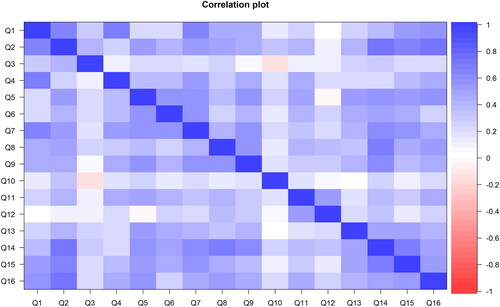
Table 2. Eigenvalue and explained variance for principal component analysis.

Component	Eigenvalue	Explained variance
		%	Cumulative%
1	6.54	40.90	40.90
2	1.42	8.87	49.77
3	1.32	8.24	58.01
4	1.21	7.59	65.60
5	1.07	6.72	72.32
6	0.89	5.60	77.92
…	…	…	…

Since we have a small number of items (16), we decided to investigate multidimensional item response theory (MIRT) models with up to 3 dimensions as recommended by parallel analysis. We will later choose the most appropriate model in an empirical way using the model comparison approaches described before. However, we simultaneously take a rationalist point of view and consider the content areas for the item (Table 1) to select the meaningful construct, and an appropriate model for that construct.

We compare three MIRT models, M2PL, M3PL, M4PL, each combined with the MGR model, with respect to their fit to the mixed-format data. The global fit statistics are reported in Table 3. Most of them support unidimensionality. They show that the M2PL + MGR model has small AIC, AICc, BIC and SABIC as compared to other models.

Table 3. Global fit statistic for each model up to 3 dimensions.

M2PL + MGR
Dimensions	p	AIC	AICc	BIC	SABIC
D1	36	3823.35	3836.60	3948.35	3834.25
D2	51	3830.24	3858.76	4007.33	3845.68
D3	65	3824.04	3873.92	4049.73	3843.71
M3PL + MGR
Dimensions	p	AIC	AICc	BIC	SABIC
D1	51	3825.61	3854.12	4002.69	3841.03
D2	66	3824.60	3876.32	4053.77	3844.57
D3	80	3824.97	3907.51	4102.75	3849.17
M4PL + MGR
Dimensions	p	AIC	AICc	BIC	SABIC
D1	66	3833.98	3885.71	4063.16	3853.95
D2	81	3824.78	3909.93	4106.03	3849.28
D3	95	3823.37	3951.81	4153.23	3852.11

$p=$ number of parameters to estimate, AIC: Akaike information criteria; AICc: Sample size corrected AIC; BIC: Bayesian information criteria; SABIC: Sample size corrected BIC. D1, D2 and D3 represent models with 1, 2 and 3 dimensions, respectively.

The likelihood ratio (LR) test is applied to compare nested models. The resulting p-values of the LR tests for nested models are presented in Table 4. The block on the left-hand side in the table compares two different models each having a specific dimension. The right-hand side block compares models with different dimensions within each of M2PL + MGR, M3PL + MGR and M4PL + MGR model. These results show that a better model fit is produced with increased dimensionality and complexity of the model. We conclude, therefore, that the unidimensionality assumption has not been met. Based on LR test results, we have observed in this study that the M4PL + MGR model fits better as compared to other models (M2PL + MGR and M3PL + MGR) because it is more complex when we fix the dimension at 2 or 3. In the case of unidimensionality, the LR test favors the 3PL + GR model as compared to other models.

Table 4. P-values for likelihood ratio tests.

	M3PL + MGR				M2PL + MGR
M2PL + MGR		D1	D2	D3		D1	D2	D3
	D1	0.0232	0.0013	0.0000	D1		0.0819	0.0013
	D2		0.0020	0.0002	D2	0.0819		0.0019
	D3			0.0157	D3	0.0013	0.0019
	M4PL + MGR				M3PL + MGR
M2PL + MGR		D1	D2	D3		D1	D2	D3
	D1	0.0144	0.0001	0.0000	D1		0.0088	0.0000
	D2		0.0002	0.0000	D2	0.0088		0.0159
	D3			0.0008	D3	0.0000	0.0159
	M4PL + MGR				M4PL + MGR
M3PL + MGR		D1	D2	D3		D1	D2	D3
	D1	0.1182	0.0007	0.0000	D1		0.0010	0.0000
	D2		0.0126	0.0008	D2	0.0010		0.0090
	D3			0.0073	D3	0.0000	0.0090

We now investigate which model (M2PL + MGR, M3PL + MGR and M4PL + MGR) is better to figure out the construct. Table 5 shows the structure of the construct for 2 and 3 factor solutions. The groups are made with the questions (items) having higher loading values in the same dimensions. Factor loading expresses the relationship of each item with underlying factor. The items with strongest association to the factor have high value of loading onto that factor. Here, we have observed that complex models with more dimensions are better to form a group of similar kind of questions as compare to other models. Moreover, the factors representing the group of items are more interpretable as compared to the factors representing the group of items in other models. So, the M4PL + MGR model is better in forming groups that are more interpretable and this result remains consistent in the comparison of models by using the LR test. The LR test supports the 3 dimensional, more complex model (M4PL + MGR) and this model is good to figure out the underlying construct of the exam. The Q₁, Q₃ and Q₄ lie in $1^{st}$ dimension. This dimension represents the students’ ability in basic statistics which include interpretation of a box plot or the definition of the term “range”. The $2^{nd}$ dimension represents Q₅, Q₆, Q₇, Q₁₁, Q₁₂ and Q₁₃. This dimension evaluates the students’ skill to solve the contingency table and hypothesis testing problem. The $3^{rd}$ construct is constituted with Q₈, Q₉, Q₁₀, Q₁₄, Q₁₅, Q₁₆ and Q₂. This dimension indicates the students’ ability in probability distribution, regression and chi-square test. The Q₂, which is a basic statistics question, is also included in the construct. Its inclusion in this dimension is debatable. One possible reason could be that students have to perform some manual calculations (e.g., calculation of standard deviation for a given sample) to answer the question, which is also required for question Q₁₄, Q₁₅ and Q₁₆.

Table 5. Two- and three-factor solution for each model.

Question	Area	M2PL + MGR		M3PL + MGR		M4PL + MGR
		D2	D3	D2	D3	D2	D3
Q 1	Basic statistics	1	3	2	2	1	1
Q 2	Basic statistics	1	1	1	3	2	3
Q 3	Basic statistics	1	1	1	3	1	1
Q4	Basic statistics (graphical)	1	3	2	2	1	1
Q5	Contingency table	1	1	1	1	1	2
Q6	Contingency table	1	1	1	1	1	2
Q7	Contingency table	1	1	2	1	1	2
Q8	Binomial distribution	1	1	1	3	2	3
Q9	Normal distribution	1	1	1	1	2	3
Q10	Normal distribution	1	1	1	1	2	3
Q11	Testing of hypothesis	2	2	2	1	1	2
Q12	Testing of hypothesis	2	2	1	1	1	2
Q13	Testing of hypothesis	1	1	1	1	1	2
Q14	Regression	1	1	1	3	2	3
Q15	Regression	1	1	1	3	2	3
Q16	Chi-square test	1	1	1	3	2	3

The questions in black color represent the $1^{st}$ factor, red the $2^{nd}$ factor and similarly green color questions represent the $3^{rd}$ factor.

4.2. Analysis using MIRT with between-item multidimensionality

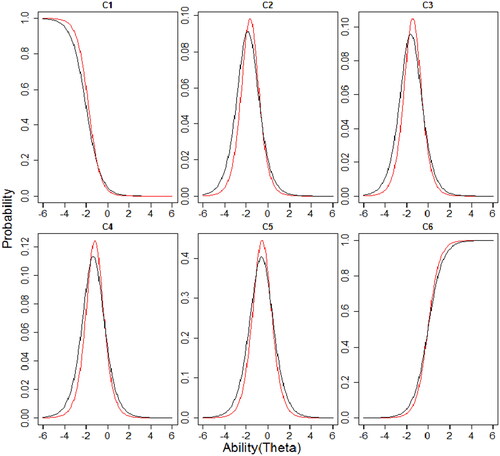
Lastly, using the dimension information from the analysis with the MIRT model before, we run now the M4PL + MGR model with 3 factors and between-item multidimensionality. This model offers the possibility for a simpler interpretation and avoids an issue of paradoxical results. Further, a possibility when using between-item multidimensionality is that we can examine how the M4PL + MGR model item response curve characterizes the items compared to unidimensional 3PL + GR model. The graphs of the item response curves of both models of each item are in Figure 3 to Figure 6. The item characteristic curve (ICC) of Q₁, Q₃ and Q₄ (factor 1; see Figure 3) in the multidimensional model with between-item multidimensionality are steeper as compared to the unidimensional model. The Q₃ and Q₄ have an upper asymptote parameter smaller than 1 in the M4PL + MGR, while Q₁ has an upper asymptote parameter close to 1 in the M4PL + MGR corresponding to the 3PL + GR. Questions Q₅, Q₆, Q₇, Q₁₁, Q₁₂ and Q₁₃ (factor 2; see Figure 4) have approximately the same ICC for both models especially if we look at ability level between -2 and 2. Slight differences in guessing parameters are visible in Q₅, Q₆, Q₁₁ and Q₁₃. While for factor 3 (see Figure 5), some ICC differ somewhat due to an upper asymptote estimate < 1 for the M4PL + MGR (Q₈, Q₉, Q₁₀ and Q₁₄), the most striking difference between the ICCs is also for this factor that the discrimination parameter is higher in the multidimensional model. Also for the graded response item Q₁₆ (see Figure 6), all categories show steeper curves for the multidimensional model. As a whole, ICCs from the between-item multidimensionality model has steeper slopes as compare to unidimensional model. This shows that items in the MIRT model with between-item multidimensionality have more discrimination power. The difficulty level of all questions are almost similar in both models except Q₁, Q₃, Q₅, Q₆ and Q₁₃ which have a slightly different difficulty level if we look at ICCs of the MIRT model and the UIRT model.

Figure 3. Item characteristic curves (ICCs) for factor 1. The black line represents the item curve of unidimensional 3PL + GR and red line represents the M4PL + MGR model.

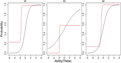
Figure 4. Item characteristic curves (ICCs) for factor 2. The black line represents the item curve of unidimensional 3PL + GR and red line represents the M4PL + MGR model.

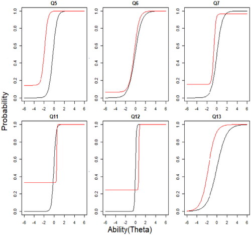
Figure 5. Item characteristic curves (ICCs) for dichotomous items in factor 3. The black line represents the item curve of unidimensional 3PL + GR and red line represents the M4PL + MGR model.

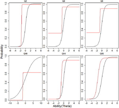
Figure 6. Item characteristic curves (ICCs) for graded response item Q₁₆. The black line represents the item curve of unidimensional 3PL + GR and red line represents the M4PL + MGR model.

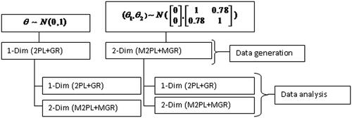
5. Simulation study

As observed in the case study in Sec. 4, the estimates for the items’ discrimination parameters are larger for the MIRT compared to the UIRT. We investigate whether this observation is generally valid and carry out a simulation study using a Monte Carlo approach. Motivated by the situation in the case study, a mixed-format data of 16 items have been generated through 300, 500 and 1000 examinees using a unidimensional and a multidimensional model. To avoid the complexity of degree of multidimensionality and to make the simulation study simpler, we have opted to investigate here a two-dimensional model with between-item multidimensionality as representant of the multidimensional models. Further, we considered 2PL models in all cases as we are here not interested in the guessing and upper asymptote parameter. In the multidimensional case we have assumed the situation in the first column of Table 5, i.e., the $2^{nd}$ dimension constitutes of items Q₁₁ and Q₁₂ and the $1^{st}$ of the other 14 items. In the two-dimensional model, we used the estimated covariance matrix (1, 0.78; 0.78, 1) from the original data as covariance for the simulation. This means that the two latent abilities ${\theta }_1$ and ${\theta }_2$ are correlated with a correlation of 0.78. As true parameter values for the simulation, we used the estimated values we got in the respective models, the 2PL + GR and the M2PL + MGR, in our case study. For data generation we had the described two models and used for data analysis both the 2PL + GR and the M2PL + MGR model for both cases, i.e., we analyzed in each case both with the correct model and the wrong model. The design of simulation study, including data generation process and data analysis method, is illustrated in Figure 7.

Figure 7. Data generation (simulation model, the true model) and data analysis (fitted model).

Data were generated and analyzed with R package mirt. For each data generation model and each considered sample size (300, 500, and 1000 students), 1000 simulation runs (repetitions) were done.

The estimated discrimination parameter was compared with the true parameter used in data generation. Root mean square error (RMSE), absolute bias (AB) and bias have then been computed for each item in each simulation run. The mean and the standard deviation of RMSE, AB and bias of the 16 items in the 1000 simulation runs was computed and is shown in Table 6.

Table 6. Simulation results for discrimination parameter (mean RMSE, AB and bias over 16 items and 1000 simulation runs) and AIC (mean over 1000 simulation runs).

		Analysis model	Discrimination parameter
True model	N		RMSE		AB		Bias		AIC
			Mean	SD	Mean	SD	Mean	SD	Mean
2PL+	300	2PL + GR	0.341	0.199	0.256	0.130	0.051	0.058	4773
GR		M2PL + MGR	0.363	0.192	0.271	0.127	0.075	0.089	4776
	500	2PL + GR	0.242	0.117	0.188	0.086	0.026	0.026	7942
		M2PL + MGR	0.260	0.115	0.203	0.086	0.047	0.073	7946
	1000	2PL + GR	0.165	0.075	0.130	0.056	0.013	0.012	15830
		M2PL + MGR	0.182	0.079	0.144	0.062	0.033	0.069	15836
M2PL+	300	2PL + GR	0.415	0.285	0.310	0.205	−0.079	0.258	4740
MGR		M2PL + MGR	0.410	0.278	0.295	0.171	0.073	0.103	4734
	500	2PL + GR	0.305	0.213	0.252	0.206	−0.061	0.254	7872
		M2PL + MGR	0.285	0.167	0.217	0.116	0.043	0.064	7860
	1000	2PL + GR	0.233	0.215	0.199	0.217	−0.075	0.252	15479
		M2PL + MGR	0.191	0.104	0.149	0.078	0.023	0.040	15468

In the $1^{st}$ block of Table 6, data were generated from the unidimensional 2PL + GR model and analyzed with 2PL + GR and confirmatory M2PL + MGR. The estimated discrimination parameters of all items are positively biased and bias reduces as the sample size increases. For each sample size the values of RMSE, AB and Bias values for M2PL + MGR model are higher compared to 2PL + GR, i.e., we obtain as expected, better values when estimating with the correct model compared to the overspecified two-dimensional model.

In the $2^{nd}$ block of Table 6, data were generated from the two-dimensional confirmatory M2PL + MGR model and analyzed with 2PL + GR and confirmatory M2PL + MGR. When analyzed with the wrong unidimensional model, the estimated discrimination parameters for the items are negatively biased. Their absolute value decreases with the increase in sample size. When analyzed with the correct two-dimensional model, the estimated discrimination parameters for the items are positively biased, decreasing with the increase in sample size. For each sample size the values of RMSE, AB and the absolute value of the mean bias are higher for the 2PL + GR model compared to M2PL + MGR, i.e., we have again better values when estimating with the correct model compared to the wrong unidimensional model.

In both the $1^{st}$ and $2^{nd}$ block of Table 6, the bias for each sample size is lower for the unidimensional model as compared to the multidimensional model. This highlights that we get higher estimated discrimination parameter in the multidimensional case as compared to unidimensional. Hence, this simulation study supports the finding of our case study that items have a higher discrimination capability in multidimensional model as compared to unidimensional model. Why is this case? When using the MIRT and considering a specific item, we obtain first a discrimination parameter estimate for each dimension. We focus then on the dimension which has the highest discrimination capacity. This means that the discrimination estimate we consider in the MIRT case is a maximum out of several estimates. It is the value which seems to belong to the ability-dimension connected to this item. Therefore, the estimate based on MIRT is larger compared to the UIRT no matter which of the models is the true one.

We have focused so far on the discrimination parameter. Looking at the results for the difficulty parameter, the results of RMSE, AB and Bias (Table 7) show only small difference between unidimensional and multidimensional. This indicates that the degree of multidimensionality seems to have no greater effect on the estimation of difficulty parameters. This result confirms the findings of Childs and Oppler (1999) and Yang (2007).

Table 7. Simulation results for difficulty parameter (mean RMSE, AB and bias over 16 items and 1000 simulation runs).

True model		Analysis model	Difficulty parameter
	N		RMSE		AB		Bias
			Mean	SD	Mean	SD	Mean	SD
2PL+	300	2PL + GR	0.336	0.299	0.244	0.182	0.063	0.096
GR		M2PL + MGR	0.343	0.302	0.248	0.184	0.078	0.100
	500	2PL + GR	0.238	0.176	0.183	0.124	0.027	0.042
		M2PL + MGR	0.242	0.178	0.185	0.125	0.041	0.046
	1000	2PL + GR	0.161	0.110	0.125	0.081	0.016	0.023
		M2PL + MGR	0.164	0.112	0.127	0.082	0.029	0.027
M2PL+	300	2PL + GR	0.332	0.279	0.243	0.175	0.049	0.087
MGR		M2PL + MGR	0.341	0.275	0.250	0.174	0.067	0.088
	500	2PL + GR	0.239	0.179	0.182	0.122	0.021	0.050
		M2PL + MGR	0.245	0.181	0.186	0.122	0.038	0.049
	1000	2PL + GR	0.161	0.103	0.127	0.079	0.017	0.022
		M2PL + MGR	0.165	0.104	0.129	0.079	0.024	0.023

In an actual study in contrast to this simulation study, we do not know if the true model is unidimensional or multidimensional. Applying the multidimensional model, even though the true is unidimensional, is safer since items can discriminate the students better and model estimated discrimination parameter are close to actual parameter, especially for large sample size as suggested by the simulation study result. Furthermore, model fit criterion AIC is only a little higher when analyzing the wrong multidimensional model when the true is unidimensional ($1^{st}$ block in Table 6). On the other hand, if we apply the wrong unidimensional model in the multidimensional case ($2^{nd}$ block in Table 6), the AIC is increased with a larger amount. The negative bias of estimated discrimination parameters is not reduced when sample size is increased to 1000. We observe, based on these results, that the violation of unidimensionality assumption may seriously bias ability and estimated item parameters which is in accordance with statements by Reckase (1979) and Harrison (1986).

6. Discussion and conclusion

In some situations, it is possible to build the model by first conducting an exploratory factor analysis and then – with new data – confirm this model. While an approach to confirm with new data would lead to strong certainty about the proposed model, we have not this possibility here: the data are too small to be split into subgroups for exploration and confirmation and due to the nature of examination in higher education, the exam will not be repeated with the same questions for new students such that no new data with the same items will be obtained in the future. In order to obtain a meaningful model in a situation like ours, we recommend to choose the model using purely data driven criteria in combination with knowledge about groups of items suspected to belong to the same factor. Models with factor structure corresponding to the areas in Table 1 are preferable. Nevertheless, it is important to carefully consider unexpected results and reflect possible explanations; in our case study, the placement of item Q₂ within another factor than it’s group Q₁ to Q₄ could be explained. This approach aims to facilitate a meaningful interpretation of our model but we point out that the resulting model still needs to be seen as exploratory.

Instead of performing a confirmatory analysis which here is difficult or impossible, we propose to conduct analyses similar to ours for several exams from different occasions (i.e., with different questions) and to look out for results which are supported from several different analyses. Based on interpretation supported by independent analyses, exams from higher education can be improved. For example, low discriminating items or items which discriminate in an ability range which is not of interest for the exam can be avoided.

The sample size in the case study appears low in the context of the applied models (e.g., 4PL) where recommendations usually require higher numbers. However, the sample size is common in higher education. Our approach described before tries to gain insights from the analysis in this challenging situation while acknowledging that results needs to be taken with care.

As we have seen in the case and simulation study, the estimates for the discrimination parameter were higher when an MIRT was used as compared to an UIRT. This effect which we explained in Sec. 5 has not found much attention in the literature yet. The estimate based on MIRT is larger compared to the UIRT no matter which of the models is the true one. This effect is important to keep in mind when working with both types of models: when one is used to a certain range of discrimination parameter estimates from UIRT analyses, one can expect a higher range when the analysis model is switched to MIRT.

An implicit assumption we made in this article is that high discriminating items are preferable. In a situation like considered here, an achievement test in higher education, it is intuitively reasonable to strive for a set of several well discriminating items with difficulties spread over a range of interest. However, in general it is not clear if high discrimination is preferable. Buyske (2005) mentions reasons to use low discriminating items in the beginning of a computerized adaptive test. To investigate a general situation in detail, we need explicitly define the objective. Then optimal design methods can formally determine the optimal item parameters, see e.g., Berger and Wong (2005).

We demonstrated in our simulation study that if it is unknown whether the UIRT or the MIRT is the underlying model it is safer to use the MIRT. We found there that if the MIRT model is used for analysis, estimated discrimination parameters are quite close to the true parameters especially for large sample size.

Based on our analysis of real data and on simulations with realistic parameter choices, we pointed out advantages of MIRT compared to UIRT. How our conclusions depend on parameter values, e.g., on the correlation between the abilities, was not in our focus here and should be investigated in future research.

Data availability

The data that support the findings of this study are available from the corresponding author (Ul Hassan) upon reasonable request.

References

- Adams, R. J., M. Wilson, and W.-C. Wang. 1997. The multidimensional random coefficients multinomial logit model. Applied Psychological Measurement 21 (1):1–23. doi:10.1177/0146621697211001.
- Baker, F. B., and S.-H. Kim. 2004. Item response theory: Parameter estimation techniques. CRC Press.
- Berger, M. P. F., and W.-K. Wong. 2005. Applied optimal designs. West Sussex: John Wiley & Sons.
- Bock, R. D., R. Gibbons, and E. Muraki. 1988. Full-information item factor analysis. Applied psychological measurement 12 (3):261–80. doi:10.1177/014662168801200305.
- Burnham, K. P., and D. R. Anderson. 2002. Model selection and multimodel inference – a practical information-theoretic approach. New York: Springer.
- Buyske, S. 2005. Optimal designs in educational testing. In Applied optimal designs, eds. M. P. F. Berger and W. K. Wong. Chichester, UK: John Wiley & Sons, Ltd.
- Chalmers, R. P. 2012. mirt: A multidimensional item response theory package for the R environment. Journal of Statistical Software 48 (6):1–29. doi:10.18637/jss.v048.i06.
- Childs, R. A., and S. H. Oppler. 1999. Practical implications of test dimensionality for item response theory calibration of the medical college admission test. MCAT Monograph. Washington, DC: ERIC.
- Conway, J. M., and A. I. Huffcutt. 2003. A review and evaluation of exploratory factor analysis practices in organizational research. Organizational Research Methods 6 (2):147–68. doi:10.1177/1094428103251541.
- De La Torre, J., and R. J. Patz. 2005. Making the most of what we have: A practical application of multidimensional item response theory in test scoring. Journal of Educational and Behavioral Statistics 30 (3):295–311. doi:10.3102/10769986030003295.
- Drasgow, F., and C. K. Parsons. 1983. Application of unidimensional item response theory models to multidimensional data. Applied Psychological Measurement 7 (2):189–99. doi:10.1177/014662168300700207.
- Fabrigar, L. R., D. T. Wegener, R. C. MacCallum, and E. J. Strahan. 1999. Evaluating the use of exploratory factor analysis in psychological research. Psychological Methods 4 (3):272–99. doi:10.1037//1082-989X.4.3.272.
- Finkelman, M., G. Hooker, and Z. Wang. 2010. Prevalence and magnitude of paradoxical results in multidimensional item response theory. Journal of Educational and Behavioral Statistics 35 (6):744–61. doi:10.3102/1076998610381402.
- Garrido, L. E., F. J. Abad, and V. Ponsoda. 2013. A new look at Horn’s parallel analysis with ordinal variables. Psychological Methods 18 (4):454–74. doi:10.1037/a0030005.
- Gorsuch, R. L. 1983. Factor analysis. 2nd ed. London: Lawrence Erlbaum Associates.
- Guttman, L. 1954. Some necessary conditions for common-factor analysis. Psychometrika 19 (2):149–61. doi:10.1007/BF02289162.
- Hambleton, R. K., H. Swaminathan, and H. J. Rogers. 1991. Fundamentals of item response theory. Newbury Park, CA: Sage Publications.
- Harrison, D. A. 1986. Robustness of IRT parameter estimation to violations of the unidimensionality assumption. Journal of Educational Statistics 11 (2):91–115. doi:10.3102/10769986011002091.
- Hartig, J., and J. Höhler. 2009. Multidimensional IRT models for the assessment of competencies. Studies in Educational Evaluation 35 (2/3):57–63. doi:10.1016/j.stueduc.2009.10.002.
- Hayton, J. C., D. G. Allen, and V. Scarpello. 2004. Factor retention decisions in exploratory factor analysis: A tutorial on parallel analysis. Organizational Research Methods 7 (2):191–205. doi:10.1177/1094428104263675.
- Henson, R. K., and J. K. Roberts. 2006. Use of exploratory factor analysis in published research common errors and some comment on improved practice. Educational and Psychological Measurement 66 (3):393–416. doi:10.1177/0013164405282485.
- Hooker, G. 2010. On separable test, correlated priors, and paradoxical results in multidimensional item response theory. Psychometrika 75 (4):694–707. doi:10.1007/s11336-010-9181-5.
- Hooker, G., M. Finkelman, and A. Schwartzman. 2009. Paradoxical results in multidimensional item response theory. Psychometrika 74 (3):419–42. doi:10.1007/s11336-009-9111-6.
- Horn, J. L. 1965. A rationale and test for the number of factors in factor analysis. Psychometrika 30 (2):179–85. doi:10.1007/BF02289447.
- Jordan, P., and M. Spiess. 2012. Generalization of paradoxical results in multidimensional item response theory. Psychometrika 77 (1):127–52. doi:10.1007/s11336-011-9243-3.
- Jordan, P., and M. Spiess. 2018. A new explanation and proof of the paradoxical scoring results in multidimensional item response models. Psychometrika 83 (4):831–46. doi:10.1007/s11336-017-9588-3.
- Kaiser, H. F. 1960. The application of electronic computers to factor analysis. Educational and Psychological Measurement 20 (1):141–51. doi:10.1177/001316446002000116.
- Kirisci, L., T.-C. Hsu, and L. Yu. 2001. Robustness of item parameter estimation programs to assumptions of unidimensionality and normality. Applied Psychological Measurement 25 (2):146–62. doi:10.1177/01466210122031975.
- Kose, I. A., and N. C. Demirtasli. 2012. Comparison of unidimensional and multidimensional models based on item response theory in terms of both variables of test length and sample size. Procedia - Social and Behavioral Sciences 46:135–40. doi:10.1016/j.sbspro.2012.05.082.
- Lee, S., and R. Terry. 2005. MDIRT-FIT: SAS macros for fitting multidimensional item response. Paper presented at the SUGI 31st Conference, Cary.
- Li, Y., H. Jiao, and R. W. Lissitz. 2012. Applying multidimensional item response theory models in validating test dimensionality: An example of k–12 large-scale science assessment. Journal of Applied Testing Technology 13 (2):1–27.
- Magis, D. 2013. A note on the item information function of the four-parameter logistic model. Applied Psychological Measurement 37 (4):304–15. doi:10.1177/0146621613475471.
- Magis, D., and G. Raîche. 2012. Random generation of response patterns under computerized adaptive testing with the r package catr. Journal of Statistical Software 48 (8):1–31. doi:10.18637/jss.v048.i08.
- Peres-Neto, P. R., D. A. Jackson, and K. M. Somers. 2005. How many principal components? Stopping rules for determining the number of non-trivial axes revisited. Computational Statistics & Data Analysis 49 (4):974–97. doi:10.1016/j.csda.2004.06.015.
- Reckase, M. D. 1979. Unifactor latent trait models applied to multifactor tests: Results and implications. Journal of Educational Statistics 4 (3):207–30. doi:10.3102/10769986004003207.
- Reckase, M. D. 1997. High dimensional analysis of the contents of an achievement test battery: Are 50 dimensions too many? Paper presented at the meeting of the Society for Multivariate Experimental Psychology, Scottsdale, AZ.
- Reckase, M. D. 2007. Multidimensional item response theory. In: Handbook of statistics 26: Psychometrics, ed. C. R. Rao and S. Sinharay, 607–42. Amsterdam, Netherlands: Elsevier.
- Reckase, M. D. 2009. Multidimensional item response theory. Springer, New York.
- Reckase, M., and X. Luo. 2015. A paradox by another name is good estimation. In Quantitative psychology research. Springer proceedings in mathematics & statistics, R. Millsap, D. Bolt, L. van der Ark, and W. C. Wang, vol. 89, 465–86. Cham: Springer.
- Reckase, M. D., and R. L. McKinley. 1991. The discriminating power of items that measure more than one dimension. Applied Psychological Measurement 15 (4):361–73. doi:10.1177/014662169101500407.
- Reckase, M. D. 1985. Models for multidimensional tests and hierarchically structured training materials. Technical report, American Coll Testing Program IOWA city IA test development div.
- Rizopoulos, D. 2006. ltm: An R package for latent variable modeling and item response theory analyses. Journal of Statistical Software 17 (5):1–25. doi:10.18637/jss.v017.i05.
- Ruscio, J., and B. Roche. 2012. Determining the number of factors to retain in an exploratory factor analysis using comparison data of known factorial structure. Psychological Assessment 24 (2):282–92. doi:10.1037/a0025697.
- Samejima, F. 1969. Estimation of latent ability using a response pattern of graded scores. Psychometrika Monograph Psychometrika 34 (4):100. doi:10.1007/BF03372160.
- Sheng, Y., and C. K. Wikle. 2007. Comparing multiunidimensional and unidimensional item response theory models. Educational and Psychological Measurement 67 (6):899–919. doi:10.1177/0013164406296977.
- Spencer, S. G. 2004. The strength of multidimensional item response theory in exploring construct space that is multidimensional and correlated. Ph. D. thesis., Doctoral Dissertation, Brigham Young University-Provo.
- van der Linden, W. J. 2012. On compensation in multidimensional response modeling. Psychometrika 77 (1):21–30. doi:10.1007/s11336-011-9237-1.
- van Rijn, P. W., and F. Rijmen. 2012. A note on explaining away and paradoxical results in multidimensional item response theory. Technical report, Princeton, New Jersey: Educational Testing Service. doi:10.1002/j.2333-8504.2012.tb02295.x.
- Velicer, W. F., C. A. Eaton, and J. L. Fava. 2000. Construct explication through factor or component analysis: A review and evaluation of alternative procedures for determining the number of factors or components. In Problems and solutions in human assessment, 41–71. Boston: Springer.
- Verma, N., and M. K. Markey. 2014. Item response analysis of Alzheimer’s disease assessment scale. In Engineering in medicine and biology society (EMBC), 2014 36th annual international conference of the IEEE, 2476–2479. Chicago: IEEE.
- Way, W. D., T. N. Ansley, and R. A. Forsyth. 1988. The comparative effects of compensatory and noncompensatory two-dimensional data on unidimensional IRT estimates. Applied Psychological Measurement 12 (3):239–52. doi:10.1177/014662168801200303.
- Wiberg, M. 2012. Can a multidimensional test be evaluated with unidimensional item response theory? Educational Research and Evaluation 18 (4):307–20. doi:10.1080/13803611.2012.670416.
- Yang, S. 2007. A comparison of unidimensional and multidimensional RASCH models using parameter estimates and fit indices when assumption of unidimensionality is violated. Ph. D. thesis, doctoral dissertation, The Ohio State University.
- Yen, W. M. 1984. Effects of local item dependence on the fit and equating performance of the three-parameter logistic model. Applied Psychological Measurement 8 (2):125–45. doi:10.1177/014662168400800201.
- Zwick, W. R., and W. F. Velicer. 1986. Comparison of five rules for determining the number of components to retain. Psychological Bulletin 99 (3):432–42. doi:10.1037//0033-2909.99.3.432.