An evaluation of a novel approach for clustering genes with dissimilar replicates

Abstract

Clustering the genes is a step in microarray studies which demands several considerations. First, the expression levels can be collected as time-series which should be accounted for appropriately. Furthermore, genes may behave differently in different biological replicates due to their genetic backgrounds. Highlighting such genes may deepen the study; however, it introduces further complexities for clustering. The third concern stems from the existence of a large amount of constant genes which demands a heavy computational burden. Finally, the number of clusters is not known in advance; therefore, a clustering algorithm should be able to recommend meaningful number of clusters. In this study, we evaluate a recently proposed clustering algorithm that promises to address these issues with a simulation study. The methodology accepts each gene as a combination of its replications and accounts for the time dependency. Furthermore, it computes cluster validation scores to suggest possible numbers of clusters. Results show that the methodology is able to find the clusters and highlight the genes with differences among the replications, separate the constant genes to reduce the computational burden, and suggest meaningful number of clusters. Furthermore, our results show that traditional distance metrics are not efficient in clustering the short time-series correctly.

Keywords:

• Clustering
• cluster validation
• microarray gene expression
• replication
• short time-series

1. Introduction

Microarrays provide information about tens of thousands of genes simultaneously through their expression levels (Schena et al. 1995) and can be used to detect the genes that contribute to the development of a disease of interest such as cancer (Richter et al., 2000; Bremnes et al. 2002; Greenman et al. 2010). It has been suggested in the literature to compare gene expression levels in a case/control study since differences in expression levels in different groups of samples indicate that such genes have an association with the disease of interest (Lewohl et al. 2000). Furthermore, it is known that genetic material may collectively contribute to the development of a disease (Peyrot et al. 2014). Therefore, investigating the co-expressed genes with microarrays may improve our knowledge on such a collective contribution. In this respect, an important step in microarray studies is grouping the genes on the basis of similarities in their expression levels (Bar-Joseph 2004). Although clustering methods have been employed to this goal (Khan et al. 1998; Sand et al. 2013; Wockner et al. 2014), there are several issues that need to be addressed carefully.

Studies such as Cho et al. (1998) and Spellman et al. (1998) followed the expression levels through time introducing the concept of time-series in microarray studies. With the introduction of time-series, researchers became able to obtain dynamic information about the genes, that has been argued to be more informative than the stable expression levels that were collected at a single time point (Bar-Joseph 2004). Then, the problem evolved into clustering the genes with respect to their similarities in their expression level profiles through time for which several well-known clustering methods, such as hierarchical clustering and self-organizing maps, have been applied (Eisen et al. 1998; Tamayo et al. 1999). These clustering methods, however, were inappropriate for clustering time-series since they ignored the dependencies between successive time points by relying on traditional distance metrics such as Euclidean distance (Irigoien, Vives, and Arenas 2011). In order to account for time dependency, numerous studies have proposed a variety of model-based methods that assume different probability distributions underlying the patterns in different clusters (Gan, Ma, and Wu 2007), for example using; autoregressive models (Ramoni, Sebastiani, and Kohane 2002); a curve-based method (Luan and Li 2004; Storey et al. 2005); a Bayesian curve-based model (Heard et al. 2005); cubic B splines (Bar-Joseph et al. 2003); methods depending on correlation coefficients (Chu et al. 1998; Heyer, Kruglyak, and Yooseph 1999); Hidden Markov Models (Schliep, Schönhuth, and Steinhoff 2003); a mixture of linear mixed models (Celeux, Martin, and Lavergne 2005; Ng et al. 2006); mathematical model based clustering (Hakamada, Okamoto, and Hanai 2006); and a parametric approach (Kim et al. 2008). However, model-based clustering methods still suffer from several drawbacks in the context of time-series microarray data. First, model-based methods may need to estimate a high number of parameters and follow distributional assumptions which might be violated in microarray data. Moreover, such methods may require prior information or reference genes to create the clusters. Last but not least, model-based methods demand a sufficient number of time points to fit the models. However, Ernst, Nau, and Bar-Joseph (2005) stated that more than 80% of the time-series microarray experiments featured less than 8 time points, which may be insufficient for model-based methods to capture the information in the data. In this respect, Ernst, Nau, and Bar-Joseph (2005) proposed a non-parametric method to cluster time-series gene expression data sets. Furthermore, Déjean et al. (2007) proposed a method that decreased the complexity of the time-series with smoothing techniques and then clustered them with hierarchical and k-means clustering, although the requirement for an appropriate distance metric still existed.

Apart from the time dependency, there are further issues to be addressed carefully in clustering short time-course gene expression data sets. First, it is common to use biological replicates in microarrays, i.e., the data collection step is reproduced on other organisms from the same species for all genes. Depending on the biological background of an organism, the genes may show different behaviors in different replicates. Such differences can improve our knowledge on the associations between the genes and the biological backgrounds of the organisms (Liang et al. 2003). Therefore, highlighting the genes which show different behaviors in different replicates is an essential part of such studies. The method proposed in Ernst, Nau, and Bar-Joseph (2005) did not address this issue; however, Irigoien, Vives, and Arenas (2011) introduced a method for clustering the gene replicates which also highlighted the genes with dissimilar replicates with a pre-filtering process. Furthermore, Cooke et al. (2011) proposed a Bayesian-based hierarchical clustering method for time-series with replicates. Another issue arises due to the large amount of constant genes that maintain their baseline expression levels throughout the study. Such genes are irrelevant to the aim of the study and usually filtered out in pre-processing to circumvent the computational burden. A variety of filtering methods for constant genes have been proposed (see Heard et al. 2005; Hackstadt and Hess 2009; Love, Huber, and Anders 2014, for examples). However, such methods have been criticized due to their subjectivity and tendency to favor unbalanced clusters (Ma et al. 2006). Finally, a common problem with the clustering methods is finding the number of clusters which is not known in advance in real data sets (Handl, Knowles, and Kell 2005; Tibshirani and Walther 2005). Although the number of clusters should be high enough to display all the patterns, very large numbers should be avoided in order to prevent redundancy. Therefore, in an optimal set of clusters the within-cluster variances should be as small as possible, whereas the between-cluster variances should be high. There are numerous cluster validation techniques that can measure the within- and between-cluster variances simultaneously and suggest an optimal number of clusters based on these similarity measures (see Bolshakova and Azuaje 2003, for a review and application of such methods on genome data).

Cinar, Ilk, and Iyigun (2018) proposed an algorithm for clustering time-series of gene expression values with potential differences between the biological replicates and compared it with several other methods. This algorithm joined the replicates of each gene consecutively and measured the distances between the genes through these joint profiles. With this approach, the algorithm aimed to project the dissimilarities between the replicates onto the gene itself. The distances between the genes were measured by considering both the magnitude and slope differences which considered the time dependencies. Furthermore, two distinct methods were implemented into the algorithm to highlight a reasonable number of clusters. In Cinar, Ilk, and Iyigun (2018), an application of this algorithm on a real data set was represented. In the present study, the proposed algorithm is evaluated on simulated data sets, where we use several factors such as sample size, the proportion of the constant genes or the genes with dissimilar replicates, and different time space patterns (evenly and unevenly separated time points). The aim of this present study is examining the effects of such factors on the algorithm while comparing the proposed method with conventional distance metrics in the literature.

2. Methodology

Let ${\mathbf{x}}_i^r$ be a row vector containing the expression values of the r^th replication $(r\in \overline{1:R})$ of gene i $(i\in \overline{1:G})$ at several time points. Another notation, ${\mathbf{x}}_{i,T(k)}^r$ represents each expression value of the r^th replication of gene i at the k^th follow up $(k\in \overline{1:K});$ thus ${\mathbf{x}}_i^r=[{\mathbf{x}}_{i,T(1)}^r,{\mathbf{x}}_{i,T(2)}^r,\dots ,{\mathbf{x}}_{i,T(K)}^r].$ Expression levels of the genes can be evenly or unevenly sampled in time in microarray experiments. T(k) denotes the time of the k^th follow up, and as the gene expressions from all the genes are measured simultaneously, the set of $[T_{(1)},T_{(2)},\dots ,T_{(k)}]$ is the same for all genes. Furthermore, we assume linear expression level changes between the successive time points. Our algorithm accepts each gene as a combination of its replicates joined successively in order to project the possible dissimilarities between the replicates of a gene onto itself which is expected to force such genes to be assigned to separate clusters. Therefore, ${\mathbf{X}}_i$ represents the combined status of the genes where ${\mathbf{X}}_i={\cup }_{r=1}^R{\mathbf{x}}_i^r.$

The distance between a pair of genes is measured with two metrics. The first metric calculates the squared Euclidean distance between the genes as follows. (1) $$d({\mathbf{X}}_i,{\mathbf{X}}_j)=\sum _{r=1}^R\sum _{k=1}^K{(x_{i,T(k)}^r-x_{j,T(k)}^r)}^2.$$(1)

As aforementioned, the methodology binds the replication of each gene consecutively by summing the squared Euclidean distances over all replications in Eq. 1(1) $$d({\mathbf{X}}_i,{\mathbf{X}}_j)=\sum _{r=1}^R\sum _{k=1}^K{(x_{i,T(k)}^r-x_{j,T(k)}^r)}^2.$$(1) and prevents an erroneous measurement to appear at the combination points of the replications. In addition to the squared Euclidean metric, Short Time Series (STS) Möller-Levet et al. (2005) measures the square of slope differences at each time interval as follows. (2) $$s({\mathbf{X}}_i,{\mathbf{X}}_j)=\sum _{r=1}^R\sum _{k=1}^{K-1}{\left[\frac{x_{i,T(k+1)}^r-x_{i,T(k)}^r}{T(k+1)-T(k)}-\frac{x_{j,T(k+1)}^r-x_{j,T(k)}^r}{T(k+1)-T(k)}\right]}^2.$$(2)

Similar to the metric described in Eq. 1(1) $$d({\mathbf{X}}_i,{\mathbf{X}}_j)=\sum _{r=1}^R\sum _{k=1}^K{(x_{i,T(k)}^r-x_{j,T(k)}^r)}^2.$$(1) , the slope differences over all replicates are summed in order to handle the replications. Eq. 2(2) $$s({\mathbf{X}}_i,{\mathbf{X}}_j)=\sum _{r=1}^R\sum _{k=1}^{K-1}{\left[\frac{x_{i,T(k+1)}^r-x_{i,T(k)}^r}{T(k+1)-T(k)}-\frac{x_{j,T(k+1)}^r-x_{j,T(k)}^r}{T(k+1)-T(k)}\right]}^2.$$(2) shows that STS distance uses the information of successive time points and relates each consecutive time point to each other; thus, it accounts for both the time dependency and time lengths.

Eqs. 1(1) $$d({\mathbf{X}}_i,{\mathbf{X}}_j)=\sum _{r=1}^R\sum _{k=1}^K{(x_{i,T(k)}^r-x_{j,T(k)}^r)}^2.$$(1) and 2(2) $$s({\mathbf{X}}_i,{\mathbf{X}}_j)=\sum _{r=1}^R\sum _{k=1}^{K-1}{\left[\frac{x_{i,T(k+1)}^r-x_{i,T(k)}^r}{T(k+1)-T(k)}-\frac{x_{j,T(k+1)}^r-x_{j,T(k)}^r}{T(k+1)-T(k)}\right]}^2.$$(2) derive two distance matrices with dimensions of G × G. Both matrices contain the distances between each pair of genes in different means. The first matrix, denoted by D, stores the distances with respect to the magnitude dissimilarities by using Eq. 1(1) $$d({\mathbf{X}}_i,{\mathbf{X}}_j)=\sum _{r=1}^R\sum _{k=1}^K{(x_{i,T(k)}^r-x_{j,T(k)}^r)}^2.$$(1) , whereas the second matrix, denoted by S, consists of the dissimilarities with respect to the shape differences by using Eq. 2(2) $$s({\mathbf{X}}_i,{\mathbf{X}}_j)=\sum _{r=1}^R\sum _{k=1}^{K-1}{\left[\frac{x_{i,T(k+1)}^r-x_{i,T(k)}^r}{T(k+1)-T(k)}-\frac{x_{j,T(k+1)}^r-x_{j,T(k)}^r}{T(k+1)-T(k)}\right]}^2.$$(2) . Then, a convex combination of these matrices is derived for a general distance matrix between each pair of genes. (3) $$\overline{\mathbf{D}}=w*\mathbf{D}+(1-w)*\mathbf{S}$$(3) where w is the user-defined parameter that can be used to assign different weights to two metrics. If w is set to a value close to 1, the algorithm emphasizes the magnitude dissimilarities, whereas values close to 0 gives more emphasis to the shape differences. In order to give equal weight to both dissimilarity characteristics, w can be set to 0.5. Finally, the values in both distance matrices are divided by the range of the measures they include before the convex combination. Therefore, the values in each matrix are standardized in the the interval of $[0,1]$ in order to prevent a possible dominance of one of the metrics over the other one.

Once the general distance matrix is derived with Eq. 3(3) $$\overline{\mathbf{D}}=w*\mathbf{D}+(1-w)*\mathbf{S}$$(3) , it is utilized as the distance matrix in the clustering. The methodology uses an agglomerative hierarchical clustering with the Ward’s distance linkage method (Szekely and Rizzo 2005). The methodology has been implemented in R programming language (R Core Team 2019) as the cgr package. The package can be found at: https://github.com/ozancinar/cgr.

Algorithm CGR creates a dendrogram tree of the genes which can be cut at any level in order to reach the desired number of clusters. As aforementioned, the set of clusters should be able to show different patterns among the genes without any redundancy. Thus, the optimal set of clusters features low within cluster variances while retaining high between cluster variances. Therefore, the optimal number of clusters can be sought via the ratio of within variance to the between variance of cluster sets with different number of clusters, where the optimal number of clusters can be obtained when this ratio is small (Yeung, Haynor, and Ruzzo 2001; Tibshirani and Walther 2005). Two cluster validation techniques have been implemented into Algorithm CGR, both of which use the same method to calculate the within cluster variances. That is, it calculates the total distance between every pair of genes for each cluster, and assigns the maximum total distance as the within cluster variance for a given number of cluster (see Eq. 4(4) $$\mathit{sum}{(\mathit{within})}_N{}_C=ma{x}_{n=1,\dots ,N_C}\left\{\sum _{i=1}^{\left|{\mathbb{C}}_n\right|}\sum _{j=1}^{\left|{\mathbb{C}}_n\right|}\overline{\mathbf{D}}({\mathbf{X}}_i,{\mathbf{X}}_j)\right\}$$(4) for sum(within)). (4) $$\mathit{sum}{(\mathit{within})}_N{}_C=ma{x}_{n=1,\dots ,N_C}\left\{\sum _{i=1}^{\left|{\mathbb{C}}_n\right|}\sum _{j=1}^{\left|{\mathbb{C}}_n\right|}\overline{\mathbf{D}}({\mathbf{X}}_i,{\mathbf{X}}_j)\right\}$$(4) where $N_C$ is the number of clusters; n is the given cluster; ${\mathbf{X}}_i$ and ${\mathbf{X}}_jϵn(i\ne j);$ $\left|{\mathbb{C}}_n\right|$ is the number of genes in cluster n.

On the other hand, the algorithm employs two methods to measure the between cluster variances. The first method extracts the smallest distance between the pair of genes from different clusters (see Eq. 5(5) $$\mathit{min}{(\mathit{between})}_N{}_C\mathrm{}=mi{n}_{n_I=1,\dots ,N_C}\left\{mi{n}_{n_J=1,\dots ,N_C}(\mathit{min}(\overline{\mathbf{D}}({\mathbf{X}}_i,{\mathbf{X}}_j)))\right\}$$(5) for min(between)). The second method calculates the average distances between every pair of genes from all pair of clusters and takes the minimum average distance (see Eq. 5(5) $$\mathit{min}{(\mathit{between})}_N{}_C\mathrm{}=mi{n}_{n_I=1,\dots ,N_C}\left\{mi{n}_{n_J=1,\dots ,N_C}(\mathit{min}(\overline{\mathbf{D}}({\mathbf{X}}_i,{\mathbf{X}}_j)))\right\}$$(5) for mean(between)). (5) $$\mathit{min}{(\mathit{between})}_N{}_C\mathrm{}=mi{n}_{n_I=1,\dots ,N_C}\left\{mi{n}_{n_J=1,\dots ,N_C}(\mathit{min}(\overline{\mathbf{D}}({\mathbf{X}}_i,{\mathbf{X}}_j)))\right\}$$(5) where N_C is the number of clusters; n_I and n_J are the given clusters $(n_I\ne n_J);$ ${\mathbf{X}}_iϵn_I$ and ${\mathbf{X}}_jϵn_J.$ (6) $$\mathit{mean}{(\mathit{between})}_N{}_C=mi{n}_{n_I=1,\dots ,N_C}\{mi{n}_{n_J=1,\dots ,N_C}(\frac{\sum _{i=1}^{\left|{\mathbb{C}}_n{}_I\right|}\sum _{j=1}^{\left|{\mathbb{C}}_n{}_J\right|}\overline{\mathbf{D}}({\mathbf{X}}_i,{\mathbf{X}}_J)}{\left|C_n{}_I\right|*\left|C_n{}_J\right|})\}$$(6) where N_C is the number of clusters; n_I and n_J are the given clusters $(n_I\ne n_J);$ ${\mathbf{X}}_iϵn_I$ and ${\mathbf{X}}_jϵn_J;$ $\left|{\mathbb{C}}_n{}_I\right|$ is the number of genes in cluster n_I and $\left|{\mathbb{C}}_n{}_J\right|$ is the number of genes in cluster n_J.

Then, the aim is searching for the set of clusters with appropriate within and between cluster variances for which the cluster validation techniques can be applied. The optimal set of clusters can be sought by observing the ratio of $\frac{\text{within}\mathrm{}\text{cluster}\mathrm{}\text{variance}}{\text{between}\mathrm{}\text{cluster}\mathrm{}\text{variance}},$ where the ratio reaches its minimum value or experiences a significant decrease between two consecutive numbers of clusters. Two validity scores can be obtained through two between cluster variances. These scores are called as VD1 and VD2 which use min(between) and mean(between), respectively.

3. Simulation setup

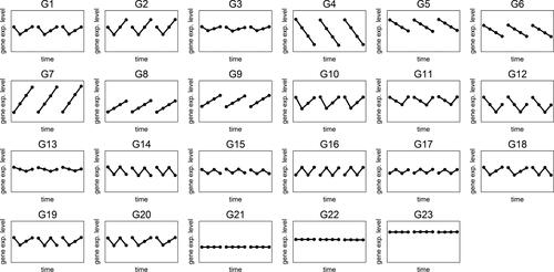
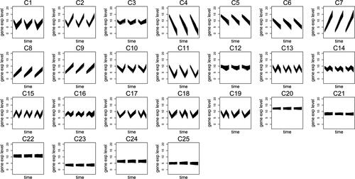
The goal in our simulations is evaluating Algorithm CGR on several issues. First, we evaluate the algorithm with regards to its performance on finding the correct clusters. Furthermore, it is also expected to separate the constant genes and the genes with dissimilar replicates into isolated clusters. Finally, it should be able to recommend meaningful number of clusters when this information is not known in advance. To this purpose, we perform a simulation study where each time-series involves 4 time points. We generate three replications for each time-series. Twenty three profiles are created which are displayed in Figure 1. We would like to direct the readers’ attention to the differences in some of the groups that are introduced to challenge the two distance metrics in our algorithm. First, we aim to challenge the Euclidean metric by adding groups with small differences, such as the patterns in G1 and G3, which has a small difference due to narrow magnitude difference at the second time point. On the other hand, we aim to challenge the slope distance metric by including similar profiles at different magnitude levels (such as the profiles in G8 and G9).

Figure 1. Twenty three profiles generated during the simulation. Each panel represents the behavior of the replications of the genes in that group. Different replications are shown with a small space between them in the panels.

In order to check the performance of the algorithm on different cases, a variety of scenarios are created by adjusting five features (each of which had two levels) shown in Table 1 in the simulation sets. With the first feature we control whether the number of genes in each group is the same or not. The second feature controls the number of genes in each group (therefore the total number of genes). With the third feature we decrease the number of genes with dissimilar replicates as such genes are not common in the real data sets and it is still important to detect them even if there are few such genes. Next, the fourth feature expands the number of constant genes in order to make the simulation set similar to a real case, since the number of constant genes may be high in real life data sets. Finally, the last feature is used to generate data sets where the time points are equally or unequally spaced.

Table 1. Five features that are used to generate different conditions in the simulation. i) The first feature controls whether the number of genes in each group is the same; ii) The second feature sets the number of genes in the group to either around or exactly 20 or 50; iii) The third feature indicates that the number of genes with dissimilar replicates is decreased to 10% of the sample sizes if it is small; iv) The fourth feature indicates that the number of constant genes is set to the total number of genes in other groups if it is set to large; v) The last feature indicates whether the time points are equally spaced; if they are, the time points are from 1 to 4 with increments of 1, whereas time points are set to 1, 4, 16 and 48 otherwise.

Feature	Levels	Abbreviations
group size	equal	ES
	unequal	US
number of genes per group	20	L
	50	H
rate of genes with different replications	large	VL
	small	VS
rate of constant genes	small	CS
	large	CL
time space	equal	ET
	unequal	UT

We use all the possible combinations of two levels of each of the five features that resulted in 32 different scenarios. In order to explain these scenarios the abbreviations shown in Table 1 are used. These scenarios are also shown with another notation, S#, where # is replaced with the order of the scenario. The orders and the explanation of the scenarios are given in Table 2.

Table 2. Scenario orders and explanations of abbreviations of the scenarios. For details see Table 1.

Scenario Order	Scenario Abbreviations	Group Size	Number of Genes	Rate of Genes with Variation in Replicates	Rate of Constant Genes	Time Spaces
S1	ES_L_VL_CS_ET	Equal	20	Large	Small	Equally Spaced
S2	ES_L_VL_CL_ET	Equal	20	Large	Large	Equally Spaced
S3	ES_L_VS_CS_ET	Equal	20	Small	Small	Equally Spaced
S4	ES_L_VS_CL_ET	Equal	20	Small	Large	Equally Spaced
S5	US_L_VL_CS_ET	Unequal	D. Unif. (10, 30)	Large	Small	Equally Spaced
S6	US_L_VL_CL_ET	Unequal	D. Unif. (10, 30)	Large	Large	Equally Spaced
S7	US_L_VS_CS_ET	Unequal	D. Unif. (10, 30)	Small	Small	Equally Spaced
S8	US_L_VS_CL_ET	Unequal	D. Unif. (10, 30)	Small	Large	Equally Spaced
S9	ES_L_VL_CS_UT	Equal	20	Large	Small	Unequally Spaced
S10	ES_L_VL_CL_UT	Equal	20	Large	Large	Unequally Spaced
S11	ES_L_VS_CS_UT	Equal	20	Small	Small	Unequally Spaced
S12	ES_L_VS_CL_UT	Equal	20	Small	Large	Unequally Spaced
S13	US_L_VL_CS_UT	Unequal	D. Unif. (10, 30)	Large	Small	Unequally Spaced
S14	US_L_VL_CL_UT	Unequal	D. Unif. (10, 30)	Large	Large	Unequally Spaced
S15	US_L_VS_CS_UT	Unequal	D. Unif. (10, 30)	Small	Small	Unequally Spaced
S16	US_L_VS_CL_UT	Unequal	D. Unif. (10, 30)	Small	Large	Unequally Spaced
S17	ES_H_VL_CS_ET	Equal	50	Large	Small	Equally Spaced
S18	ES_H_VL_CL_ET	Equal	50	Large	Large	Equally Spaced
S19	ES_H_VS_CS_ET	Equal	50	Small	Small	Equally Spaced
S20	ES_H_VS_CL_ET	Equal	50	Small	Large	Equally Spaced
S21	US_H_VL_CS_ET	Unequal	D. Unif. (40, 60)	Large	Small	Equally Spaced
S22	US_H_VL_CL_ET	Unequal	D. Unif. (40, 60)	Large	Large	Equally Spaced
S23	US_H_VS_CS_ET	Unequal	D. Unif. (40, 60)	Small	Small	Equally Spaced
S24	US_H_VS_CL_ET	Unequal	D. Unif. (40, 60)	Small	Large	Equally Spaced
S25	ES_H_VL_CS_UT	Equal	50	Large	Small	Unequally Spaced
S26	ES_H_VL_CL_UT	Equal	50	Large	Large	Unequally Spaced
S27	ES_H_VS_CS_UT	Equal	50	Small	Small	Unequally Spaced
S28	ES_H_VS_CL_UT	Equal	50	Small	Large	Unequally Spaced
S29	US_H_VL_CS_UT	Unequal	D. Unif. (40, 60)	Large	Small	Unequally Spaced
S30	US_H_VL_CL_UT	Unequal	D. Unif. (40, 60)	Large	Large	Unequally Spaced
S31	US_H_VS_CS_UT	Unequal	D. Unif. (40, 60)	Small	Small	Unequally Spaced
S32	US_H_VS_CL_UT	Unequal	D. Unif. (40, 60)	Small	Large	Unequally Spaced

One thousand simulation sets for each of the 32 scenarios are generated and average misclustered gene rate in each scenario is calculated in order to evaluate Algorithm CGR. Misclustered genes are defined by the following procedure: First, the majority of the groups are detected in each cluster which is decided by the group with the most frequent genes in a cluster. Next, the genes which are not from the group that is majority in a cluster are counted as misclustered genes. Finally, we use five different w selections which are 0, 0.25, 0.5, 0.75 and 1, to see the effect of various weight selections. These five selections are denoted as $S\#.1,S\#.2,S\#.3,S\#.4,$ and $S\#.5,$ respectively in Table 3.

Table 3. Average misclustering rates.

	* = 1	* = 2	* = 3	* = 4	* = 5		* = 1	* = 2	* = 3	* = 4	* = 5
S1.*	0.17	0.00	0.00	0.03	0.06	S17.*	0.17	0.00	0.00	0.02	0.05
S2.*	0.38	0.00	0.00	0.00	0.03	S18.*	0.38	0.00	0.00	0.00	0.02
S3.*	0.18	0.00	0.00	0.04	0.07	S19.*	0.18	0.00	0.00	0.02	0.06
S4.*	0.39	0.00	0.00	0.00	0.03	S20.*	0.39	0.00	0.00	0.00	0.03
S5.*	0.17	0.00	0.00	0.03	0.06	S21.*	0.17	0.00	0.00	0.02	0.05
S6.*	0.38	0.00	0.00	0.00	0.05	S22.*	0.38	0.00	0.00	0.00	0.03
S7.*	0.18	0.00	0.00	0.04	0.07	S23.*	0.18	0.00	0.00	0.02	0.05
S8.*	0.39	0.00	0.00	0.00	0.05	S24.*	0.39	0.00	0.00	0.00	0.03
S9.*	0.21	0.00	0.01	0.04	0.06	S25.*	0.22	0.00	0.00	0.03	0.05
S10.*	0.41	0.00	0.00	0.01	0.03	S26.*	0.41	0.00	0.00	0.00	0.02
S11.*	0.23	0.01	0.01	0.04	0.07	S27.*	0.24	0.00	0.00	0.04	0.06
S12.*	0.41	0.01	0.00	0.01	0.03	S28.*	0.42	0.00	0.00	0.00	0.03
S13.*	0.22	0.02	0.01	0.04	0.06	S29.*	0.22	0.00	0.00	0.03	0.05
S14.*	0.41	0.01	0.00	0.01	0.05	S30.*	0.41	0.00	0.00	0.00	0.03
S15.*	0.24	0.03	0.02	0.04	0.07	S31.*	0.24	0.01	0.00	0.03	0.05
S16.*	0.42	0.02	0.01	0.01	0.05	S32.*	0.42	0.01	0.00	0.00	0.03

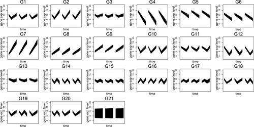
In order to evaluate the performance of cluster validation techniques described in Sec. 2, we generate another data set based on the scenarios described above. As aforementioned, genes rarely show dissimilar replicates in a real life case; thus, their proportion are generally smaller compared to the number of genes which feature similar replicates. Moreover, the constant genes can appear at any magnitude level and their number is expected to be large compared to the other genes assuming that a filtering process has not been performed prior to clustering. In order to achieve a data set to examine the performance of our algorithm, we let the constant genes in S24 to scatter over the range of data set. The time-series that are generated in this examination are displayed in Figure 2.

Figure 2. Time-series generated for the simulation data set which is used for evaluating the cluster validation techniques.

Finally, in order to compare the distance metric used in Algorithm CGR with conventional distance metrics, we cluster the data sets generated in our simulations with the distance metrics provided in the R programming language. The hclust() function provides the hierarchical clustering in R utilizing a distance matrix which can be derived by the dist() function. The dist() function provides Euclidean, Maximum, Manhattan, Canberra and Minkowski metrics (Deza and Deza 2009); therefore, we derive the dendograms using these distance metrics and compare the performance of Algorithm CGR with the performances of other distance metrics using the correct number of clusters in the simulation.

4. Results

4.1. Evaluation of algorithm CGR

Table 3 presents the overall misclustering rates for each scenario with five weight selections. The highest misclustering rates are observed when only the shape metric is used, due to the fact that the constant genes are not separated successfully from each other by this metric alone. This leads to even higher misclustering rates in even numbered scenarios since the number of constant genes is expanded in these scenarios. Furthermore, paired comparison analyses with respect to the sample size show that Algorithm CGR results in lower misclustering rates for large samples except for the cases where only the shape metric is used.

In any weight selection except for cases where $*=5,$ unequally spaced time points result in significantly higher misclustering rates. The misclustering rates change between 0.17 and 0.42 in cases where the shape metric is ignored. However, when the shape metric is incorporated, the misclustering rates decrease dramatically where the highest misclustering rates are 0.03, 0.02, and 0.04 for w = 0.25, 0.50, and 0.75, respectively. Moreover, there are no differences between equally and unequally spaced scenarios for the cases where only distance metric is used, since the time pattern is ignored when the shape metric is not included. On the other hand, the highest average misclustering rates are 0.07 for both equally and unequally spaced time points when only the shape metric is used, which is slightly higher than the weight selections of 0.25, 0.50, and 0.75.

The performance of Algorithm CGR in separating the constant genes is evaluated with several measures. Correct classification rates for detecting the constant genes vary between 95.4% and 100% among all scenarios. The lowest correct classification rate is obtained in S19 and S27 when only the distance metric is utilized. The average correct classification rates for each weight selection are 100%, 100%, 99.9%, 98.4% and 96.5% for five weight selections, respectively. Furthermore, sensitivity of detecting the constant genes varies in 71% and 100% while specificity is between 94% and 100%. Paired comparisons show that the algorithm performs better with regards to sensitivity with large sample sizes where the average sensitivity scores are 92.2% and 99.9% for small and large samples, respectively. With regards to specificity, however, the algorithm performs better with small samples. However, the difference here is negligible; the specificity for small samples is 99.5%, whereas it is 98.8% for the big samples.

Algorithm CGR is successful in separating the genes with dissimilar replicates in 46.25% of the scenarios. The lowest correct classification rate is observed in S26 where both the proportion of the genes with dissimilar replicates and the constant genes are large. When only the shape metric is used in this scenario, the algorithm results in 98.1% correct classification rate. Similarly, sensitivity scores change between 99.6% and 100%. A pairwise t-test between the VS and VL sets shows that there is a significant difference in sensitivity of detecting the genes with dissimilar replicates. Sensitivity is slightly higher when the proportion of the genes with dissimilar replicates is small. Furthermore, a statistically significant difference is found with a pairwise t-test between the average specificity scores in VL and VS sets. Specificity decreases to 96.5% from 99.3% when the VS cases are compared to their respective VL sets.

Since the Algorithm CGR is based on hierarchical clustering approach, its behavior in terms of time complexity is similar to hierarchical clustering. Computation time is not dependent on the distance metric used but it depends on the number of genes to be clustered.

4.2. Evaluation of cluster validation techniques

Algorithm CGR is employed on the data set displayed in Figure 2 with equal weights for both metrics. Following the clustering, the validation techniques explained in Sec. 2 are then utilized on the clustering results. The validation scores are displayed in Figure 3.

Figure 3. Validation score graphs for the data set shown in Figure 2.

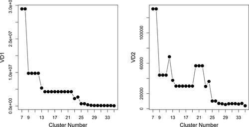
Both validation scores highlight noticeable decreases up to the set of 13 clusters. Furthermore, both methods indicate a convergence in the validation scores after 23 clusters. Second validation score demonstrates an increase between 25 and 26 clusters which is probably due to a separation of a correct cluster into redundant clusters which leads to a decrease in the between cluster variation. Therefore, the interpretation is that both validation scores indicate that the number of clusters in the data might be between 23 and 25. Figure 4 displays the partition of the data into 23 clusters.

Figure 4. 23 clusters obtained from the data set in Figure 2.

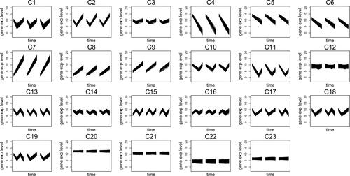
Algorithm CGR is able to separate the three groups including the genes with dissimilar replicates (from C17 to C19) by separating the data into 23 clusters (Figure 4). Furthermore, it also divides the constant genes into four clusters between C20 and C23 separately from the non-constant genes. Unlikely to the scenarios in the previous simulation, the constant genes do not have any specific magnitude level; thus, the number of clusters that should be assigned to the constant genes is not known in advance. However, Algorithm CGR successfully separates them from the non-constant genes. However, the algorithm fails to detect all individual patterns in the first 17 groups shown in Figure 2 with 23 clusters. For instance, G1 and G10 (which show a slight difference in their expression levels at the second time point) are clustered together in C1. Furthermore, C3 includes the genes from G3 and G13 where the algorithm misses their minimum levels at different time points. Due to these problems and that the validation scores suggest cluster numbers between 23 and 25, we increase the number of clusters to 24 (see Figure 5).

Figure 5. 24 clusters obtained from the data set in Figure 2.

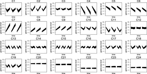
One of the problems we face with 23 clusters is avoided when the data is separated into 24 clusters. Specifically, G1 and G10 are separated from each other and clustered in C1 and C10, respectively. On the other hand, C3 still involves patterns from G3 and G13. Therefore, the number of clusters is increased to 25, the last number suggested by the validation scores (Figure 6). Then, Algorithm CGR successfully detects all the patterns in the simulation set into clusters from C1 to C16 while separating the genes with dissimilar replicates (C17 - C19) and the constant genes (C20 - C25).

Figure 6. 25 clusters obtained from the data set in Figure 2.

4.3. Comparison with other distance metrics

Finally, we compare Algorithm CGR with conventional distance metrics provided in R. Figure 7 displays the misclustering rates of Algorithm CGR along with other distance metrics with box-plots derived from all the scenarios. Our results show that Algorithm CGR have lower misclustering rates than the conventional distance metrics in general. Specifically, when both metrics described in eqs. 1(1) $$d({\mathbf{X}}_i,{\mathbf{X}}_j)=\sum _{r=1}^R\sum _{k=1}^K{(x_{i,T(k)}^r-x_{j,T(k)}^r)}^2.$$(1) and 2(2) $$s({\mathbf{X}}_i,{\mathbf{X}}_j)=\sum _{r=1}^R\sum _{k=1}^{K-1}{\left[\frac{x_{i,T(k+1)}^r-x_{i,T(k)}^r}{T(k+1)-T(k)}-\frac{x_{j,T(k+1)}^r-x_{j,T(k)}^r}{T(k+1)-T(k)}\right]}^2.$$(2) are incorporated together with different weights such that w is set to 0.25, 0.50 or 0.75, Algorithm CGR results in substantially lower misclustering rates than other selections.

Figure 7. Misclustering rate comparison between different distance metrics over all the scenarios. The first three box-plots represent Algorithm CGR with different weight selections. The remaining box-plots represent the misclustering rates of conventional distance metrics provided in the R programming language.

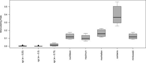
Similar to the results with misclustering rates, the conventional distance metrics do not perform as well as the distance metric provided in Algorithm CGR. The false positive rates for detecting the constant genes show that Algorithm CGR produce false positive rates below 0.026 when both distance metrics are incorporated with different weights, whereas the conventional distance metrics result in false positive rates between 0.097 and 0.251. The differences between methods are lower with regards to detecting the genes with dissimilar replicates. Algorithm CGR has a false positive rate of below 0.002 in detecting the genes with dissimilar replicates regardless of the weight selection. Among the conventional methods, maximum distance is able to detect such genes with a negligible amount (i.e., almost 0) of false positive rate. Among the rest of the metrics, Euclidean and Minkowski metrics receive a false positive rate of 0.032, while Manhattan and Canberra metrics have a false positive rate above 0.157.

5. Discussion

Clustering gene expression values that have been collected in the form of short time-series requires careful consideration of several issues. Namely, the dependencies among the measurements taken at different time points are ignored by most of the conventional distance metrics. Furthermore, possible differences between replicates may occur due to their biological differences. Finally, the existence of high number of constant genes inflates the computation time.

Cinar, Ilk, and Iyigun (2018) proposed an algorithm, Algorithm CGR, to cluster short time-series gene expression data sets which accounts for aforementioned issues by incorporating two well-known distance metrics on different replicates separately. In this study, we evaluate the performance of this algorithm on simulated data sets and compare it with conventional methods. Our results show that incorporating multiple distance metrics can provide clustering results with lower misclustering rates. Specifically, when the two distance metrics are used with equal weights, Algorithm CGR provides clusters with substantially lower misclustering rates than the conventional methods. We also observe that using only one of the distance metrics may fail to detect different clusters (Table 3). For example, when only the shape metric is used, genes with similar patterns at different magnitudes are not separated correctly, which in turn inflates the misclustering rate. Therefore, the combination of two metrics, even with different weights, is very beneficial for getting the results with low misclustering rates, and Algorithm CGR is successful in clustering the time-series when both metrics are included. Furthermore, our comparisons with the conventional distance metrics, such as Euclidean and Minkowski, also emphasize the importance of mixing different types of distance metrics as implemented in Algorithm CGR, since conventional distance metrics result in higher misclustering rates compared to Algorithm CGR. Moreover, the conventional distance metrics are usually not able to detect the genes with dissimilar replicates or the constant genes.

Furthermore, Algorithm CGR is able to highlight the genes which display different patterns in their biological replicates by clustering them in separate clusters even when the number of such genes is decreased during the simulation. Similarly, Algorithm CGR successfully detects and separates the constant genes into different clusters which suggests that Algorithm CGR could be useful when the constant genes are not filtered completely. Finally, the clustering validation scores that are provided in the same algorithm are able to highlight meaningful number of clusters which can provide aid to the researchers when this information is not known in advance.

6. Conclusion

In this paper, the performance of a novel clustering algorithm, Algorithm CGR, is evaluated for the time-series microarray data. The algorithm is evaluated under several simulation studies with different conditions. We observe that the algorithm can find the correct clusters especially as the number of genes increases for both equally and unequally spaced time points. Additionally, accuracy measures indicate that the algorithm could highlight the genes with dissimilar replicates and isolate the constant genes. Finally, evaluation of the cluster validation scores proposed in this study shows that the algorithm is also successful in finding the patterns, detecting the genes with dissimilar replicates and isolating the constant genes in a data set where the number of clusters is not known in advance.

References

- Bar-Joseph, Z. 2004. Analyzing time series gene expression data. Bioinformatics (Oxford, England) 20 (16):2493–503. doi:10.1093/bioinformatics/bth283.
- Bar-Joseph, Z., G. K. Gerber, D. K. Gifford, T. S. Jaakkola, and I. Simon. 2003. Continuous representations of time-series gene expression data. Journal of Computational Biology : A Journal of Computational Molecular Cell Biology 10 (3-4):341–56. doi:10.1089/10665270360688057.
- Bolshakova, N., and F. Azuaje. 2003. Cluster validation techniques for genome expression data. Signal Processing 83 (4):825–33.
- Bremnes, R., R. Veve, E. Gabrielson, F. R. Hirsch, A. Baron, L. Bemis, R. M. Gemmill, H. A. Drabkin, and W. A. Franklin. 2002. High-throughput tissue microarray analysis used to evaluate biology and prognostic significance of the e-cadherin pathway in non-small-cell lung cancer. Journal of Clinical Oncology: Official Journal of the American Society of Clinical Oncology 20 (10):2417–28. doi:10.1200/JCO.2002.08.159.
- Celeux, G., O. Martin, and C. Lavergne. 2005. Mixture of linear mixed models for clustering gene expression profiles from repeated microarray experiments. Statistical Modelling: An International Journal 5 (3):243–67.
- Cho, R. J., M. J. Campbell, E. A. Winzeler, L. Steinmetz, A. Conway, L. Wodicka, T. G. Wolfsberg, A. E. Gabrielian, D. Landsman, D. J. Lockhart, et al. 1998. A genome-wide transcriptional analysis of the mitotic cell cycle. Molecular Cell 2 (1):65–73.
- Chu, S., J. DeRisi, M. Eisen, J. Mulholland, D. Botstein, P. O. Brown, and I. Herskowitz. 1998. The transcriptional program of sporulation in budding yeast. Science (New York, N.Y.) 282 (5389):699–705. doi:10.1126/science.282.5389.699.
- Cinar, O., O. Ilk, and C. Iyigun. 2018. Clustering of short time-course gene expression data with dissimilar replicates. Annals of Operations Research 263 (1-2):405–28.
- Cooke, E. J., R. S. Savage, P. D. Kirk, R. Darkins, and D. L. Wild. 2011. Bayesian hierarchical clustering for microarray time series data with replicates and outlier measurements. BMC Bioinformatics 12 (1):399 doi:10.1186/1471-2105-12-399.
- Core Team, R. 2019. R: A Language and Environment for Statistical Computing. Vienna, Austria: R Foundation for Statistical Computing.
- Déjean, S., P. G. Martin, A. Baccini, and P. Besse. 2007. Clustering time-series gene expression data using smoothing spline derivatives. EURASIP Journal on Bioinformatics and Systems Biology 2007 (1):1–10.
- Deza, M. M., and E. Deza. 2009. Encyclopedia of distances. In Encyclopedia of distances, 1–583. Berlin, Heidelberg: Springer.
- Eisen, M. B., P. T. Spellman, P. O. Brown, and D. Botstein. 1998. Cluster analysis and display of genome-wide expression patterns. Proceedings of the National Academy of Sciences of the United States of America 95 (25):14863–8. doi:10.1073/pnas.95.25.14863.
- Ernst, J., G. J. Nau, and Z. Bar-Joseph. 2005. Clustering short time series gene expression data. Bioinformatics 21 (Suppl 1):i159–i168.
- Gan, G., C. Ma, and J. Wu. 2007. Data clustering: Theory, algorithms, and applications. Philadelphia, PA: SIAM; Alexandria, VA: ASA.
- Greenman, C. D., G. Bignell, A. Butler, S. Edkins, J. Hinton, D. Beare, S. Swamy, T. Santarius, L. Chen, S. Widaa, et al. 2010. Picnic: an algorithm to predict absolute allelic copy number variation with microarray cancer data. Biostatistics (Oxford, England) 11 (1):164–75. doi:10.1093/biostatistics/kxp045.
- Hackstadt, A. J., and A. M. Hess. 2009. Filtering for increased power for microarray data analysis. BMC Bioinformatics 10 (1):11. doi:10.1186/1471-2105-10-11.
- Hakamada, K., M. Okamoto, and T. Hanai. 2006. Novel technique for preprocessing high dimensional time-course data from dna microarray: Mathematical model-based clustering. Bioinformatics (Oxford, England) 22 (7):843–8. doi:10.1093/bioinformatics/btl016.
- Handl, J., J. Knowles, and D. B. Kell. 2005. Computational cluster validation in post-genomic data analysis. Bioinformatics (Oxford, England) 21 (15):3201–12. doi:10.1093/bioinformatics/bti517.
- Heard, N. A., C. C. Holmes, D. A. Stephens, D. J. Hand, and G. Dimopoulos. 2005. Bayesian coclustering of anopheles gene expression time series: Study of immune defense response to multiple experimental challenges. Proceedings of the National Academy of Sciences of the United States of America 102 (47):16939–44. doi:10.1073/pnas.0408393102.
- Heyer, L. J., S. Kruglyak, and S. Yooseph. 1999. Exploring expression data: Identification and analysis of coexpressed genes. Genome Research 9 (11):1106–15. doi:10.1101/gr.9.11.1106.
- Irigoien, I.,. S. Vives, and C. Arenas. 2011. Microarray time course experiments: Finding profiles. IEEE/ACM Transactions on Computational Biology and Bioinformatics 8 (2):464–75. doi:10.1109/TCBB.2009.79.
- Khan, J., R. Simon, M. Bittner, Y. Chen, S. B. Leighon, T. Pohida, P. D. Smith, Y. Jiang, G. C. Gooden, J. M. Trent, et al. 1998. Gene expression profiling of alveolar rhabdomyosarcoma with cdna microarrays. Genetics 180 (2):821–34.
- Kim, B. R., L. Zhang, A. Berg, J. Fan, and R. Wu. 2008. A computational approach to the functional clustering of periodic gene-expression profiles. Genetics 180 (2):821–34. doi:10.1534/genetics.108.093690.
- Lewohl, J. M., L. Wang, M. F. Miles, L. Zhang, P. R. Dodd, and R. A. Harris. 2000. Gene expression in human alcoholism: Microarray analysis of frontal cortex. Alcoholism: Clinical and Experimental Research 24 (12):1873–82. doi:10.1111/j.1530-0277.2000.tb01993.x.
- Liang, M., A. G. Briggs, E. Rute, A. S. Greene, and A. W. Cowley. 2003. Quantitative assessment of the importance of dye switching and biological replication in cdna microarray studies. Physiological Genomics 14 (3):199–207. doi:10.1152/physiolgenomics.00143.2002.
- Love, M. I., W. Huber, and S. Anders. 2014. Moderated estimation of fold change and dispersion for rna-seq data with DESeq2. Genome Biology 15 (12):550 doi:10.1186/s13059-014-0550-8.
- Luan, Y., and H. Li. 2004. Model-based methods for identifying periodically expressed genes based on time course microarray gene expression data. Bioinformatics (Oxford, England) 20 (3):332–9. doi:10.1093/bioinformatics/btg413.
- Ma, P., C. I. Castillo-Davis, W. Zhong, and J. S. Liu. 2006. A data-driven clustering method for time course gene expression data. Nucleic Acids Res 34 (4):1261–9. doi:10.1093/nar/gkl013.
- Möller-Levet, C. S., F. Klawonn, K.-H. Cho, H. Yin, and O. Wolkenhauer. 2005. Clustering of unevenly sampled gene expression time-series data. Fuzzy Sets and Systems 152 (1):49–66.
- Ng, S. K., G. J. McLachlan, K. Wang, L. B. T. Jones, and S. Ng. 2006. A mixture model with random-effects components for clustering correlated gene-expression profiles. Bioinformatics (Oxford, England) 22 (14):1745–52. doi:10.1093/bioinformatics/btl165.
- Peyrot, W. J., Y. Milaneschi, A. Abdellaoui, P. F. Sullivan, J. J. Hottenga, D. I. Boomsma, and B. W. Penninx. 2014. Effect of polygenic risk scores on depression in childhood trauma. The British Journal of Psychiatry : The Journal of Mental Science 205 (2):113–9. doi:10.1192/bjp.bp.113.143081.
- Ramoni, M. F., P. Sebastiani, and I. S. Kohane. 2002. Cluster analysis of gene expression dynamics. Proceedings of the National Academy of Sciences of the United States of America 99 (14):9121–6. doi:10.1073/pnas.132656399.
- Richter, J., U. Wagner, J. Kononen, A. Fijan, J. Bruderer, U. Schmid, D. Ackerman, R. Maurer, G. Alund, H. Knönagel, et al. 2000. High-throughput tissue microarray analysis of cyclin e gene amplification and overexpression in urinary bladder cancer. The American Journal of Pathology 157 (3):787–94.
- Sand, M., M. Skrygan, D. Sand, D. Georgas, T. Gambichler, S. A. Hahn, P. Altmeyer, and F. G. Bechara. 2013. Comparative microarray analysis of microrna expression profiles in primary cutaneous malignant melanoma, cutaneous malignant melanoma metastases, and benign melanocytic nevi. Cell and Tissue Research 351 (1):85–98. doi:10.1007/s00441-012-1514-5.
- Schena, M., D. Shalon, R. W. Davis, and P. O. Brown. 1995. Quantitative monitoring of gene expression patterns with a complementary dna microarray. Science (New York, N.Y.) 270 (5235):467–70. doi:10.1126/science.270.5235.467.
- Schliep, A., A. Schönhuth, and C. Steinhoff. 2003. Using hidden markov models to analyze gene expression time course data. Bioinformatics 19 (Suppl 1):i255–i263.
- Spellman, P. T., G. Sherlock, M. Q. Zhang, V. R. Iyer, K. Anders, M. B. Eisen, P. O. Brown, D. Botstein, and B. Futcher. 1998. Comprehensive identification of cell cycle-regulated genes of the yeast saccharomyces cerevisiae by microarray hybridization. Molecular Biology of the Cell 9 (12):3273–97. doi:10.1091/mbc.9.12.3273.
- Storey, J. D., W. Xiao, J. T. Leek, R. G. Tompkins, and R. W. Davis. 2005. Significance analysis of time course microarray experiments. Proceedings of the National Academy of Sciences of the United States of America 102 (36):12837–42. doi:10.1073/pnas.0504609102.
- Szekely, G. J., and M. L. Rizzo. 2005. Hierarchical clustering via joint between-within distances: Extending ward’s minimum variance method. Journal of Classification 22 (2):151–83.
- Tamayo, P., D. Slonim, J. Mesirov, Q. Zhu, S. Kitareewan, E. Dmitrovsky, E. S. Lander, and T. R. Golub. 1999. Interpreting patterns of gene expression with self-organizing maps: Methods and application to hematopoietic differentiation. Proceedings of the National Academy of Sciences of the United States of America 96 (6):2907–12. doi:10.1073/pnas.96.6.2907.
- Tibshirani, R., and G. Walther. 2005. Cluster validation by prediction strength. Journal of Computational and Graphical Statistics 14 (3):511–28.
- Wockner, L. F., E. P. Noble, B. R. Lawford, R. M. Young, C. P. Morris, V. L. J. Whitehall, and J. Voisey. 2014. Genome-wide dna methylation analysis of human brain tissue from schizophrenia patients. Translational Psychiatry 4 (1):e339 doi:10.1038/tp.2013.111.
- Yeung, K. Y., D. R. Haynor, and W. L. Ruzzo. 2001. Validating clustering for gene expression data. Bioinformatics (Oxford, England) 17 (4):309–18. doi:10.1093/bioinformatics/17.4.309.