A comparison of statistical methods for age-specific reference values of discrete scales

Abstract

Age-specific reference values are important in medical science to evaluate the normal ranges of subjects and to help physicians signal potential disorders as early as possible. They are applied to many types of measurements, including discrete measures obtained from questionnaires and clinical tests. These discrete measures are typically skewed to the left and bounded by a maximum score of one (or 100%). This article investigates the performances of various statistical methods, including quantile regression, the Lambda-Mu-Sigma (LMS) method and its extensions, and the generalized additive models for location, scale, and shape with zero and one-inflated distributions implemented with either fractional polynomials or splines, for age-specific reference values on discrete measures. Their large-sample performances were investigated using Monte-Carlo simulations, and the consistency of splines and fractional polynomials age profiles with quantile regression had been demonstrated as well. The advantages and disadvantages of these methods were illustrated with data on the Infant Motor Profile, a test score on motor behavior in children of 3–18 months. We concluded that quantile regression with fractional polynomials approach is a robust and computationally efficient method for setting age-specific reference values for discrete measures.

Keywords:

• Fractional polynomial
• LMS method
• Quantile regression
• GAMLSS

1. Introduction

Age-specific reference values (also known as (per)centile or quantile curves) are broadly used in medical sciences, in particular in research fields such as obstetrics and pediatrics, where development over time is of particular importance. As the curves describe expected “normal” development (growth, or any other measured quantity showing development over time), they serve a special purpose in the early detection of deviation from typical development, indicating possible problems at an early stage and hence enabling extra monitoring or early intervention where necessary.

In the construction of such curves, the statistical challenge lies in creating best fitting continuous reference centiles that change smoothly over time by using the most appropriate statistical method available on the one hand, while simultaneously keeping the models used as simple to apply and interpret as possible, and losing as little as possible in terms of quality and reliability of results on the other hand (Silverwood and Cole 2007). The most basic approach is known as the “mean and standard deviation (SD) model,” applicable in the case where data are normally distributed and where the variance is independent of the time-metric (Cole 2012). As this assumption is hardly ever valid, the last decades showed the development of numerous more advanced statistical approaches, based on both cross-sectional and longitudinal data.

Ideally, growth charts used for detecting atypical patterns from multiple measurements over time should take the past into account and should, therefore, be based on longitudinal data (Wei and He 2006). An example of a growth curve model that accounts for within-subject dependence in longitudinal data is the conditional quantile regression model for continuous responses (Geraci and Bottai 2014). Although more methodological advances have been recently made in this area, applications of these methods are not often encountered, nor easily done (see Thompson’s comments of Wei and He (2006)). Moreover, in practice and especially in the case of less commonly used outcome variables, cross-sectional data are generally more often available than appropriate longitudinal data. Therefore, in this article, we will focus on the construction of centile curves for cross-sectional and non-normally (discrete, skewed, and with ceiling effect) distributed data only.

In 2006, a group of statisticians in the commission of the World Health Organization presented a thorough overview and review of all available (at that time 30) statistical methods for constructing growth curves (Borghi et al. 2006). In this extensive review, eventually, five methods were proposed for the construction of children’s growth curves. Three were extensions or variations of the LMS Box-Cox approach (Cole and Green 1992), using both non-parametric and parametric functions of age, and including fractional polynomials (FPs) (Royston and Wright 1998). In the footsteps of this WHO review, identical statistical models were recommended and adopted for the development of fetal and newborn growth standards in a more recent study (Altman et al. 2013; Papageorghiou et al. 2014).

Nowadays, two general relatively simple approaches can be distinguished in the estimation of quantiles of unknown skewed distributions: variations of quantile regression (Koenker and Hallock 2001), which may accommodate specific ceiling effects and skewness very easily, and variations of the LMS method, which might offer – when correctly specified – better estimation precision than quantile regression (Wei and He 2006). Quantile regression is a non-parametric approach capable of modeling quantiles of a dependent outcome variable as a function of independent explanatory variables or covariates from a cross-sectional data set. It is especially useful in the case where it is difficult to find an appropriate transformation for data after which normality could be assumed. The LMS method is a semi-parametric approach that has been developed for the estimation of age-related quantiles of skewed distributions. It essentially standardizes and transforms the outcome variable using a Box-Cox transformation, such that its distribution would resemble the normal distribution more closely. Recent developments have further extended the LMS Box-Cox approach to consider the generalization of the normal distribution to other distributions to incorporate skewness and kurtosis. In the present study, in addition to the original LMS, we also considered the Student t distribution (LMST) (Rigby and Stasinopoulos 2006) and the power exponential distribution (LMSP) (Rigby and Stasinopoulos 2004) which includes normal, Laplace, and uniform distributions as special cases.¹ Nevertheless, the LMS Box-Cox approach with different distributional assumptions (namely, the LMS, LMST, and LMSP) can be viewed as special cases of the more general class of Generalized Additive Models for Location, Scale and Shape (GAMLSS, Rigby and Stasinopoulos (2005)) models.

In the original LMS method proposed by Cole and Green, the mean (M), standard deviation (S), and Box-Cox transformation power (L) are all modeled as functions of age with these functions approximated by cubic splines (Cole and Green 1992). Penalties are imposed on the likelihood based on the squared second derivative of the L, M, S curves to strike the balance between “fidelity to the data” and “the smoothness of the curves.” These splines can adapt perfectly to data locally but may lead to local non-monotone parts of the curves at any point of the age period, whenever small artifacts in data would be present. These smoothing issues may be more pronounced for discrete outcome variables. Alternatively, the use of FPs in the context of growth curves has proven its usefulness already in applications by clinicians from various research fields, such as obstetrics and gynecology (Tilling et al. 2014), gene expression studies in clinical genetics (Tan et al. 2011) and cognitive function of children (Ryoo et al. 2017). Therefore, we also considered FP age profiles in combination with the LMS method and quantile regression. When responses are restricted to $[0,1]$ or any other finite interval, the appropriateness of the LMS method is questionable, since it does not restrict the range of the response. Alternatively, it has been suggested by other authors to consider zero and one inflated distributions such as the inflated logit skew Student t distribution (ILSST) and the inflated beta distribution (IB) in the GAMLSS class (Hossain et al. 2016).

Currently, it is unknown which of the three aforementioned methods (quantile regression, LMS, or the inflated distributions) would perform better in estimating age-specific reference values for item-based scores or similar types of discrete, skewed, and bounded data. Moreover, our case study, discussed in the next section, shows that the use of these methods applied on a relatively small empirical data set do not provide similar age-specific curves and a simulation study comparing the methods is warranted. The measure of comparison in the simulation study is the proportion of correctly estimated reference values and we will investigate the large sample properties using large cross-sectional data sets.

2. Motivating example on motor behavior in young children

2.1. Introduction of the infant motor profile

Assessment of motor behavior of infants older than 3 months is difficult, but it has become increasingly clear that the quality of motor behavior plays a quintessential role. In fact, until recently with the introduction of the Infant Motor Profile (IMP) by Heineman, Bos, and Hadders-Algra (2008) and Heineman et al. 2018), no good measure existed to measure the quality of motor behavior in infants older than 3 months. The IMP is a qualitative assessment, and it measures five different domains of motor behavior in children of 3–18 months old. The domains represent the size of motor repertoire (variation), ability to select motor strategies from the repertoire (adaptability), movement fluency, movement symmetry, and motor performance. To obtain IMP scores on each domain, an examiner assesses a video recording of approximately 15 min of self-produced motor behavior of a child – consisting of sitting, reaching, and grasping among other things. The examiner uses a list of K = 80 discrete items in total, which the examiner should score. At certain ages though, not all items may be applicable, since the children are not yet capable of performing this motor behavior. The items of one particular domain j of a subject i are then used in the following way to calculate the total IMP score for that domain: $S_{ij}=K_{ij}^{-1}{\sum }_{k=1}^{K_{ij}}{M}_{jk}^{-1}{X}_{\mathit{ijk}}$ with $X_{\mathit{ijk}}\in \{1,\dots ,M_{jk}\}$ the score of item k for subject i in domain j, K_ij the number of (non-missing) items applicable to subject i in domain j, M_jk the maximum attainable score of item k in domain j. The total IMP score, which represents the overall performance for motor behavior, is calculated as the average of the domain-specific scores, i.e., $y_i=5^{-1}{\sum }_{j=1}^5{S}_{ij}.$ Note that each domain-specific score S_ij and the total IMP score y_i are discrete measures with values in the interval $(0,1].$

The total IMP score would make it possible to detect and evaluate motor disorders at an early stage when age-specific normal or reference values for the general population of infants would exist since it would be expected that children with motor disorders would have deviating IMP scores on at least one domain. Reference values could be determined by sampling infants at random from the general population and assessing their IMP scores. Calculating age-specific quantiles for the IMP scores is not straightforward since the IMP scores would typically not behave according to a normal distribution or any other well-known continuous parametric distribution. Besides the fact that individual domain scores will be discrete, a substantial amount of children may score the maximum value of 1 for a few domains, while other children may typically provide relatively low scores. This results in a skewed discrete distribution function for the individual domain scores. Additionally, the number of (in)applicable items for a subject varies between subjects, which makes both X_ijk and K_ij random and the distribution of S_ij less tractable. Although several flexible statistical methods for estimating age-specific reference values exist, e.g., parametric and non-parametric quantile regression, the ILSST and the LMS method, it is not obvious which method would be most suitable for age-specific reference values on the IMP scores.

2.2. Data, resampling, and evaluation measure

Data consisted of two different studies. One study was a cross-sectional study of 115 young children from the infant welfare centers in the north of the Netherlands. These children were measured at one of the five predetermined time points (4, 6, 10, 12, or 18 months). The second study was a longitudinal study of 30 young children recruited from colleagues and acquaintances of researchers of the University Medical Center Groningen (UMCG) with follow-up times at 3, 4, 5, 6, 8, 10, 12, 15, and 18 months. Thus, the combined data set is a mixed data set with 145 children. Since we apply analysis techniques for cross-sectional data, we created cross-sectional data sets using random sampling (without replacement). For each subject from the longitudinal study, one observation of the existing follow-up times was selected at random. This sampling approach was performed 500 times and we fitted the quantile regression, the LMS method, and the ILSST method with splines and FP to all 500 sampled data sets. More details on the methods can be found in Sec. 3.

To determine the best polynomial form of the FPs, we chose the combination of power values that would minimize the average goodness-of-fit criterion over the 500 resampled data sets. For quantile regression, we used the objective function instead of the goodness-of-fit criterion (see Sec. 3). For both LMS and ILSST approaches, the Akaike information criterion (AIC) with a correction for small sample sizes was considered. Furthermore, we took a sequential approach to select the optimal FP for both LMS and ILSST methods. First, the optimal FP for the mean μ was selected (using no FP for standard deviation and skewness), then the optimal FP for standard deviation σ was selected (using the optimal powers for the FP of the mean μ and no FP for skewness) and finally, the optimal FP for skewness was selected (using the optimal powers for the FP of the mean μ and the standard deviation σ). In this sequential approach, the optimal powers are sequentially determined, but the parameter estimates of the FP for μ and σ change in each step. After the optimal FP has been determined, a model with this optimal FP was fitted to each of the 500 resampled data sets and the parameter estimates of the corresponding optimal FP were taken as the average over all of them.

To determine the best splines, we again used a goodness-of-fit criterion over the resampled data sets. For quantile regression, the value of the objective function was again used and for LMS and ILSST the generalized AIC (GAIC) was used, which is obtained by adding a fixed penalty (the effective degrees of freedom) to the global deviance (see Rigby and Stasinopoulos (2005) for more details). However, a different approach from what we used for FP was taken to determine the appropriate pooled quantiles for the splines. The quantiles were first calculated for each resampled data set given the best model selected for that particular data set. Then, the final quantiles were taken as the averaged quantiles over all resampled data sets. Note that, for all spline approaches, a monotonicity constraint was enforced. For quantile regression, the monotonicity constraints were considered for each quantile separately. For both LMS and ILSST, the monotonicity constraints were restricted on the parameter μ only. This is because in theory children cannot degenerate in motor behavior.

For each resampled data, using the best model² of each distribution, we compared different distributions using the Bayesian information criterion (BIC). One single best distribution was selected using majority voting (i.e., more than half the times) over the 500 resampled data. Method-wise comparisons were made only considering the besting-fitting distribution for each method.

To find out how well the estimated models would fit the complete data set, we used the following performance measures. At each age of 3, 4, 5, 6, 8, 10, 12, 15, and 18 months we calculated the proportion of observations outside the estimated quantiles. We also calculated the percentage of children that had one or more observations outside the estimated quantiles at any of the ages. The estimated quantiles of interest were at 2.5%, 5.0%, 95.0%, and 97.5%. For the lower reference values, we expect to find proportions equal to the quantiles, and for the upper reference values, we expect a proportion equal to one minus the quantile. Finally, we also compared the estimated reference ranges between the methods.

2.3. Statistical analysis results

For the LMS, the normal distribution is the best fitting distribution according to the majority voting results (see Supplementary material) while the logit skewed Student t distribution is better compared to the beta distribution. Therefore, we focused on the discussions of LMS (with normal distribution) and the ILSST model below.

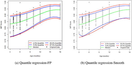
The best power values for the second-degree FP used in quantile regression were $p_1=p_2=3$ for all quantiles, except for the 5% quantile. For the quantile at 5% nominal level, the best power value $p_1=p_2=-2$ provided the lowest objective function value in quantile regression. However, this led to inconsistencies between the 5% quantile and the 2.5% quantile. To be more specific, when the optimal FP ($p_1=p_2=-2$) was selected for quantile at 5%, the estimated 5% quantiles at the age period 8–12 months would fall below the estimated quantile at 2.5%. This contradicts the ordering of quantiles. In principle, the optimal FP should not be selected for each quantile separately but should be selected in combination with other quantiles to obtain consistent results. Therefore, we chose the power values of $p_1=p_2=3$ for the 5% quantile in lieu of the optimal FP. Note that the FP with $p_1=p_2=3$ was still among the top five best power values for the 5% quantile. The resulting quantiles are provided in Figure 1(a). The estimated quantiles of quantile regression with spline functions are provided in Figure 1(b). The quantiles using splines were very similar to the ones obtained by the FP at the 2.5%, 50%, 95%, and 97.5% level. It had the same problem as the FP approach at the 5% quantiles. However, it lacks the flexibility of the FP for adjustment. With the aberrant behavior of the 5% quantile, it is unclear how to adjust using the information obtained from other quantiles.

Figure 1. The average 2.5%, 5%, 50%, 95%, and 97.5% quantile curve estimates over the 500 sampled data sets each fitted with a quantile regression overlay on the original data of the 145 children. (a) Quantile regression-FP. (b) Quantile regression-Smooth.

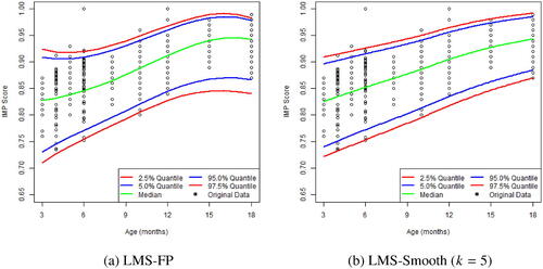
The best power values for the LMS method with FP were $p_1=p_2=3$ for μ, $p_1=0$ for σ, $p_1=3$ for λ. The corresponding quantiles estimated by the best FP are shown in Figure 2(a). For the splines, we fitted the model with the penalties k in the GAIC ranging from 2 to 5. Note that, when k = 5 GAIC is effectively BIC for the sampled data since the value is approximately the natural logarithm of the sample size 145. The resulting quantile estimates with different values of k can be found in the supplementary material. We discovered that the quantile curves were quite “wiggly” for small values of k. We believe that the smaller values of k demonstrate an overfitting (see Supplementary material). Therefore, we chose the most conservative penalty for smoothing. With the choice of k = 5, it produced close to linear smooth quantile curves as shown in Figure 2(b).

Figure 2. The average 2.5%, 5%, 50%, 95%, and 97.5% quantile curve estimates over the 500 sampled data sets each fitted with the LMS method overlay on the original data of the 145 children. (a) LMS-FP. (b) LMS-Smooth (k = 5) .

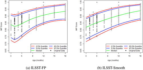
For the ILSST methods, the best power values for the FP were found to be $p_1=-2,p_2=0,p_1=3,p_1=1,$ and $p_1=-2$ for parameter μ, σ, ν, and p, respectively. We considered τ to be independent of the age a priori. The estimated quantiles were found to be highly influenced by data at the young age of 3 and 4 months (see Figure 3(a)). On the other hand, due to the monotonicity constraints, the spline approach was quite robust to these effects which had an approximately linear relationship between the quantiles and the age over the age range of 3 and 4 months (see Figure 3(b)).

Figure 3. The average 2.5%, 5%, 50%, 95%, and 97.5% quantile curve estimates over the 500 sampled data sets each fitted with the ILSST method overlay on the original data of the 145 children. (a) ILSST-FP. (b) ILSST-Smooth.

2.4. Evaluation of age-specific curves

To compare the different methods, Tables 1–3 show the percentages of observations from the original data set outside the estimated quantiles for each age separately and combined, respectively. Tables 1–3 also report the percentage of children that have one or more observations outside the reference values.

Table 1. Performance measurements for quantile regression (QR) (Subjects*: Percentage of children that had one or more observations outside the age-specific reference curves).

		QR-FP				QR-Smooth
Age	N	$<2.5\%$	$<5\%$	$>95\%$	$>97.5\%$	$<2.5\%$	$<5\%$	$>95\%$	$>97.5\%$
3	30	0.00%	0.00%	0.00%	0.00%	0.00%	0.00%	0.00%	0.00%
4	52	3.85%	5.77%	1.92%	1.92%	3.85%	3.85%	1.92%	1.92%
5	29	0.00%	0.00%	10.34%	6.90%	0.00%	0.00%	10.34%	6.90%
6	55	1.82%	3.64%	14.55%	7.27%	1.82%	3.64%	14.55%	7.27%
8	29	0.00%	0.00%	0.00%	0.00%	0.00%	0.00%	0.00%	0.00%
10	56	1.79%	3.57%	5.36%	1.79%	3.57%	3.57%	5.36%	1.79%
12	59	0.00%	1.69%	3.39%	3.39%	0.00%	1.69%	3.39%	3.39%
15	30	0.00%	0.00%	3.33%	0.00%	0.00%	0.00%	6.67%	0.00%
18	60	1.67%	6.67%	5.00%	3.33%	1.67%	1.67%	5.00%	3.33%
Total	400	1.25%	3.00%	5.25%	3.00%	1.50%	2.00%	5.50%	3.00%
Subjects*	145	3.42%	8.22%	10.96%	7.53%	4.11%	5.48%	11.64%	7.53%

Table 2. Performance measurements for the LMS method (Subjects*: Percentage of children that had one or more observations outside the age-specific reference curves).

		LMS-FP				LMS-Smooth
Age	N	< 2.5%	< 5%	> 95%	> 97.5%	< 2.5%	< 5%	> 95%	> 97.5%
3	30	0.00%	0.00%	0.00%	0.00%	0.00%	0.00%	0.00%	0.00%
4	52	0.00%	5.77%	1.92%	0.00%	0.00%	7.69%	1.92%	0.00%
5	29	0.00%	0.00%	6.90%	3.45%	0.00%	0.00%	6.90%	3.45%
6	55	1.82%	3.64%	7.27%	7.27%	1.82%	3.64%	7.27%	1.82%
8	29	0.00%	0.00%	0.00%	0.00%	0.00%	0.00%	0.00%	0.00%
10	56	1.79%	3.57%	1.79%	1.79%	0.00%	3.57%	1.79%	1.79%
12	59	0.00%	1.69%	3.39%	3.39%	0.00%	0.00%	3.39%	3.39%
15	30	0.00%	0.00%	0.00%	0.00%	0.00%	0.00%	3.33%	0.00%
18	60	0.00%	0.00%	5.00%	3.33%	1.67%	6.67%	3.33%	0.00%
Total	400	0.50%	2.00%	3.25%	2.50%	0.50%	3.00%	3.25%	1.25%
Subjects	145	1.37%	5.48%	8.22%	6.16%	1.37%	8.22%	8.22%	3.42%

Table 3. Performance measurements for the ILSST method (Subjects*: Percentage of children that had one or more observations outside the age-specific reference curves).

		ILSST-FP				ILSST-Smooth
Age	N	< 2.5%	< 5%	> 95%	> 97.5%	< 2.5%	< 5%	> 95%	> 97.5%
3	30	0.00%	0.00%	0.00%	0.00%	0.00%	0.00%	0.00%	0.00%
4	52	0.00%	0.00%	1.92%	1.92%	0.00%	7.69%	1.92%	1.92%
5	29	0.00%	0.00%	6.90%	3.45%	0.00%	0.00%	6.90%	3.45%
6	55	0.00%	3.64%	7.27%	1.82%	1.82%	3.64%	7.27%	1.82%
8	29	0.00%	0.00%	0.00%	0.00%	0.00%	0.00%	0.00%	0.00%
10	56	3.57%	5.36%	1.79%	1.79%	1.79%	3.57%	1.79%	1.79%
12	59	1.69%	3.39%	3.39%	3.39%	0.00%	1.69%	3.39%	3.39%
15	30	0.00%	0.00%	3.33%	3.33%	0.00%	0.00%	3.33%	3.33%
18	60	1.67%	1.67%	3.33%	3.33%	1.67%	6.67%	3.33%	3.33%
Total	400	1.00%	2.00%	3.25%	2.25%	0.75%	3.25%	3.25%	2.25%
Subjects	145	2.74%	5.48%	8.22%	6.16%	2.05%	8.90%	8.22%	6.16%

The two approaches with quantile regression provide almost identical performance measures, except for the quantiles at 2.5% for children at 10 months old and at 97.5% for children at 18 months old. It can be seen from Table 1 that quantile regression provides reasonable reference level values at the upper limits while the lower limits are conservative. The number of subjects with a value outside the reference range is liberal overall, especially at the higher part of the reference range. This is to be expected when individual observations at specific ages fall outside the curves with percentages close to nominal.

Both LMS with FP and splines perform similar overall but differ among specific age ranges. The LMS with FP is conservative at the lower limits of the reference ranges, while the upper limits have close to nominal values. Meanwhile, LMS with splines has conservative estimates of the quantiles overall reference levels. The percentages of children with a value outside the reference values are reasonably close to the nominal value, although they are mainly liberal except for the 2.5% quantiles. Comparing the LMS method with the quantile regression method shows that the latter performs better at all quantiles but similar at the 5% quantiles.

The ILSST approaches perform almost identical to the LMS approaches, but it has a better reference value at the 2.5% quantile, although still conservative. Overall, the ILSST methods have conservative reference values except for the 97.5% quantile which is close to the nominal values. Furthermore, the results from the FP approach and the spline approach are consistent. The percentages of subjects outside the reference range are also very similar to those from the LMS methods.

The quantile regression appears to perform slightly better than the other two alternatives, although all three methods have reference values close to nominal. No clear differences in terms of the performance measurements are observed between the FP approach and the spline approach. However, with quantile regression, FP seems to provide more reasonable quantiles at the lower age range than splines do, while with LMS and ILSST this is the other way around. Quantile regression with FP also provides opportunities to deal with the problem of crossing quantiles by using one unified best power value for FP across different quantiles. For quantile regression with splines, this is less straightforward to adjust in practice.

3. Statistical methods for age-specific reference curves

In this section, we will discuss the quantile regression, the LMS, and the ILSST approaches. We will explain how smooth age profiles can be constructed with these methods using FPs and splines. We will refer to the literature for more details when needed.

3.1. Quantile regression

Details on the method of quantile regression for cross-sectional data sets are described by Koenker and Hallock (2001). In essence, the optimization technique used for quantile regression looks a lot like the way that we would normally optimize a regression function with least squares. For least squares regression, we would solve the following expression: $$\underset{\mu \in \mathbb{R}}{\arg \min }\sum _{i=1}^n{\left(y_i-\mu \right)}^2,$$ to obtain an estimate of the unconditional mean μ (the sample mean), while for quantile regression we would solve the following (1) $$\underset{\xi \in \mathbb{R}}{\arg \min }\sum _{i=1}^n{\rho }_{\alpha }\left(y_i-\xi \right),$$(1) where y_i is the outcome measure (e.g., the total IMP score), ${\rho }_{\alpha }$ is the tilted absolute value function that yields the α^th sample quantile as its solution, ξ the α-quantile of the distribution of y_i, and n is the number of subjects or observations. The function ${\rho }_{\alpha }$ is defined by $${\rho }_{\alpha }(u)=\{\begin{array}{ll}\alpha u\hfill & \text{if }u\ge 0\hfill \\ (\alpha -1)u\hfill & \text{otherwise}.\hfill \end{array}$$

In this analysis, only one parameter or scalar was optimized (μ for the least squares approach and ξ for the quantile regression method), but we would also like these scalars to depend on one or several covariates, similar to multiple linear regression. For least squares regression, this can be simply implemented by replacing the scalar μ by a parametric function defined as $\mu (x_i,\beta ),$ with x_i a vector of covariates for subject i and β a vector of unknown parameters. The function $\mu (x,\beta )$ is typically linear in the parameters. There is no restriction to do the same for quantile regression, i.e., replace ξ by a function $\xi (x_i,\beta )$ in (1)(1) $$\underset{\xi \in \mathbb{R}}{\arg \min }\sum _{i=1}^n{\rho }_{\alpha }\left(y_i-\xi \right),$$(1) . This replaces (1)(1) $$\underset{\xi \in \mathbb{R}}{\arg \min }\sum _{i=1}^n{\rho }_{\alpha }\left(y_i-\xi \right),$$(1) by the following expression (the objective function) (2) $$\underset{\beta \in \mathbb{R}}{\arg \min }\sum _{i=1}^n{\rho }_{\alpha }\left(y_i-\xi \left(x_i,\beta \right)\right).$$(2)

For the scores of motor behavior, the response y_i for subject i in quantile regression is either the total IMP score S_i, or possibly the score S_ij of one of the domains j for a child i at age t_i and the vector of covariates x_i would at least contain the age t_i of child i.

3.2. The LMS method

For a particular response y_i of subject i, the LMS method uses three parameters in the Box-Cox transformation: the mean μ, the standard deviation σ, and a power parameter λ (Cole and Green 1992). The transformed observation z_i is now given by (3) $$z_i=\{\begin{array}{cc}\left[{(y_i/{\mu }_i)}^{{\lambda }_i}-1\right]/({\lambda }_i{\sigma }_i)\hfill & \text{if}\mathrm{ }{\lambda }_i\ne 0\hfill \\ \hspace{0.17em}\text{log}\hspace{0.17em}(y_i/{\mu }_i)/{\sigma }_i\hfill & \text{if}\mathrm{ }{\lambda }_i=0\hfill \end{array}$$(3) with μ_i, σ_i, and λ_i the subject-specific parameters. The LMS method was used to generate age-related reference values, by considering smoothed curves for the three parameters λ_i, μ_i, and σ_i, as function of age. This means that Cole and Green (1992) implemented ${\lambda }_i=\lambda (t_i),{\mu }_i=\mu (t_i),$ and ${\sigma }_i=\sigma (t_i)$ in (3)(3) $$z_i=\{\begin{array}{cc}\left[{(y_i/{\mu }_i)}^{{\lambda }_i}-1\right]/({\lambda }_i{\sigma }_i)\hfill & \text{if}\mathrm{ }{\lambda }_i\ne 0\hfill \\ \hspace{0.17em}\text{log}\hspace{0.17em}(y_i/{\mu }_i)/{\sigma }_i\hfill & \text{if}\mathrm{ }{\lambda }_i=0\hfill \end{array}$$(3) for subject i, with $\lambda (t),\mu (t),$ and $\sigma (t)$ smooth functions of age t.

To determine reference values, it is assumed that the transformed observation z_i has a particular distribution (e.g., normal distribution, Student t distribution, and power exponential distribution). Using the quantiles $Z_{\alpha }$ of this distribution and by taking the inverse of the transformation in (3)(3) $$z_i=\{\begin{array}{cc}\left[{(y_i/{\mu }_i)}^{{\lambda }_i}-1\right]/({\lambda }_i{\sigma }_i)\hfill & \text{if}\mathrm{ }{\lambda }_i\ne 0\hfill \\ \hspace{0.17em}\text{log}\hspace{0.17em}(y_i/{\mu }_i)/{\sigma }_i\hfill & \text{if}\mathrm{ }{\lambda }_i=0\hfill \end{array}$$(3) , we can find an equation for the αth quantile of the distribution of y_i at age t. The age-related quantiles are given by the next expression. (4) $$C_{100\alpha }(t)=\{\begin{array}{cc}\mu \left(t\right){\left(1+\lambda (t)\sigma (t)Z_{\alpha }\right)}^{1/\lambda (t)}\hfill & \text{if}\mathrm{ }\lambda \left(t\right)\ne 0\hfill \\ \mu \left(t\right)\hspace{0.17em}\text{exp}\hspace{0.17em}\left(\sigma (t)Z_{\alpha }\right)\hfill & \text{if}\mathrm{ }\lambda \left(t\right)=0\hfill \end{array}$$(4)

The LMS method can be considered as a particular case in a more general model specification employed in the GAMLSS framework. It assumes that the conditional distribution of the response variable y_i given x_i follows certain p-parameter distribution $F({\theta }_{i1},\dots ,{\theta }_{ip})$ with (5) $$g_k({\theta }_{ik})={\xi }_k(x_i,\beta ),$$(5) for $k=1,\dots ,p$ where g_k and ξ_k are the link function and smooth function, respectively. The LMS method can be equivalently written in such form with $g_1({\mu }_i)={\mu }_i$ (identity link), $g_2({\sigma }_i)=\hspace{0.17em}\text{log}\hspace{0.17em}{\sigma }_i,$ and $g_3({\lambda }_i)={\lambda }_i,$ and a resulting distribution that is named the Box-Cox Cole and Green (BCCG) distribution (Stasinopoulos et al. 2017).³

3.3. The ILSST and the IB method

The ILSST method incorporates support at 0 and 1 by assuming a different distribution with inflated 0 and 1 as following: (6) $$f_Y(y_i|{\mu }_i,{\sigma }_i,{\nu }_i,{\tau }_i,p_i,q_i)=\{\begin{array}{cc}(1-p_i-q_i)f_W(w_i|{\mu }_i,{\sigma }_i,{\nu }_i,{\tau }_i)\hfill & \text{if}\mathrm{ }0<y_i<1\hfill \\ p_i\hfill & \text{if}\mathrm{ }{y}_i=1\hfill \\ q_i\hfill & \text{if}\mathrm{ }{y}_i=0\hfill \end{array},$$(6) where $f_W(w|\mu ,\sigma ,\nu ,\tau )$ is a distribution of interests (skewed Student t distribution or beta distribution). More specifically, for the skewed Student t distribution, $f_W(w|\mu ,\sigma ,\nu ,\tau )$ is a logit transformed variable with probability density function (7) $$f_W(w|\mu ,\sigma ,\nu ,\tau )=\frac{c}{\sigma }\left\{1+\frac{{(w-\mu )}^2}{\tau {\sigma }^2}\left[{\nu }^2\mathrm{⊮}(w<\mu )+\frac{1}{{\nu }^2}\mathrm{⊮}(w\ge \mu )\right]\right\}$$(7) for $-\infty <w<\infty ,$ where $c=2\nu {\left[(1+{\nu }^2)B(1/2,\tau /2){\tau }^{1/2}\right]}^{-1}$ (B is the beta function). Note that here μ represents the mode of W (Fernández and Steel 1998). The link functions relate the parameters $({\mu }_i,{\sigma }_i,{\nu }_i,{\tau }_i,p_i,q_i)$ to the smooth functions of x_i given by (8) $$\begin{array}{cc}{\mu }_i\hfill & ={\xi }_1(x_i)\hfill \\ \hspace{0.17em}\text{log}\hspace{0.17em}({\sigma }_i)\hfill & ={\xi }_2(x_i)\hfill \\ \hspace{0.17em}\text{log}\hspace{0.17em}({\nu }_i)\hfill & ={\xi }_3(x_i)\hfill \\ \hspace{0.17em}\text{log}\hspace{0.17em}(\tau -2)\hfill & ={\xi }_4(x_i)\hfill \\ \hspace{0.17em}\text{log}\hspace{0.17em}\left(\frac{p_i}{1-p_i}\right)\hfill & ={\xi }_5(x_i)\hfill \\ \hspace{0.17em}\text{log}\hspace{0.17em}\left(\frac{q_i}{1-q_i}\right)\hfill & ={\xi }_6(x_i).\hfill \end{array}$$(8)

For the beta distribution, w = y with probability density function $$f_W(w_i|a_i,b_i)=\frac{1}{B(a_i,b_i)}{w}_i^{a_i-1}{(1-w_i)}^{b_i-1}$$ where ${\mu }_i=a_i/(a_i+b_i)$ and ${\sigma }_i={(1/(a_i+b_i+1))}^{1/2}.$ The link functions relate the parameters $({\mu }_i,{\sigma }_i,p_i,q_i)$ given by (8).

3.4. Smooth functions of the linear predictors

In the literature, both parametric (e.g., polynomials) and non-parametric (e.g., splines) approaches have been proposed for constructing smooth functions of the linear predictors (see, e.g., Andersen and Skovgaard 2010).

3.4.1. Penalized splines

Cole and Green (1992) originally used third-degree B-splines (cubic splines) with penalty defined in terms of the square of the second derivative (O’Sullivan 1986, 1988) for each of the $\lambda (t),\mu (t),$ and $\sigma (t)$ terms described in Sec. 3.2. That is, their objective function is given by $$\mathcal{\ell }-\frac{1}{2}{\alpha }_{\lambda }\int {\left[\lambda ″(t)\right]}^{2}dt-\frac{1}{2}{\alpha }_{\mu }\int {\left[\mu ″(t)\right]}^{2}dt-\frac{1}{2}{\alpha }_{\sigma }\int {\left[\sigma ″(t)\right]}^{2}dt,$$ where $\mathcal{\ell }$ is the log-likelihood function derived from (3)(3) $$z_i=\{\begin{array}{cc}\left[{(y_i/{\mu }_i)}^{{\lambda }_i}-1\right]/({\lambda }_i{\sigma }_i)\hfill & \text{if}\mathrm{ }{\lambda }_i\ne 0\hfill \\ \hspace{0.17em}\text{log}\hspace{0.17em}(y_i/{\mu }_i)/{\sigma }_i\hfill & \text{if}\mathrm{ }{\lambda }_i=0\hfill \end{array}$$(3) , and ${\alpha }_{\lambda },{\alpha }_{\mu },{\alpha }_{\sigma }$ are smoothing parameters. And the L, M, S curves are further specified as a linear combination of a set of n third-degree B-splines $B_j(t_i;3)$ as $$\lambda (t_i)=\sum _{j=1}^n{b}_{\lambda j}{B}_j(t_i;3);\hspace{1em}\mu (t_i)=\sum _{j=1}^n{b}_{\mu j}{B}_j(t_i;3);\hspace{1em}\sigma (t_i)=\sum _{j=1}^n{b}_{\sigma j}{B}_j(t_i;3).$$

Instead of using the second derivative of the L, M, and S curve as the penalty term, lower or higher order might be used as well. However, higher derivatives become too complex to formulate exactly. Eilers and Marx (1996) simplified and generalized O’Sullivan’s approach by using a difference penalty on the coefficients of adjacent B-splines. These are called P-splines. P-splines have useful properties such as preserving moments of data and their behavior with a strong penalty gives a connection to polynomial models. For quantile regression, Koenker, Ng, and Portnoy (1994) made a similar simplification to the original L²-norm of the second derivative but with the absolute value of the second derivatives (L¹-norm) for computational feasibility. This means that the original objective function in (2) for quantile regression is now penalized as $$\sum _i{\rho }_{\tau }\{y_i-\xi (x_i,\beta )\}+\kappa {\int }_0^1|\xi ″(x,\beta )|dx,$$ with $\xi (x,\beta )={\sum }_{j=1}^n{\beta }_j{B}_j(x;3)$ and κ the smoothing parameter.

In case of the IMP example, it is natural to consider the motor behavior (i.e., the IMP score) of a child to not decrease over time. To take such constraints into account, say in the M curve of the LMS method, we wish to impose monotonicity restrictions on the B-splines. This is achieved by adding an additional asymmetric penalty on the first-order differences according to Bollaerts, Eilers, and Aerts (2006). For instance, to ensure the positiveness of the first derivative of the linear predictor in the quantile regression with P-splines, an additional penalty term ${\sum }_{j=2}^n{w}_j{({\beta }_j-{\beta }_{j-1})}^2$ is added to the objective function, where $$w_j=\{\begin{array}{cc}0\hfill & \text{if}\mathrm{ }{\beta }_j-{\beta }_{j-1}\ge 0\hfill \\ 1\hfill & \text{otherwise}\hfill \end{array}$$ are weights that penalize the objective function for values of β_j that violates the monotonicity constraint.

3.4.2. Fractional polynomials

Conventional polynomials provide a simple parametric approach to approximate the curves but typically require a large number of terms to successfully capture the complexities that arise in experimental data. Besides, polynomials tend to produce artifacts such as “end effects” in higher-order fitted curves. Alternatively, Royston and Altman (1994) introduced an extended family of polynomial functions, which they termed “fractional polynomials” for modeling curved relationships. FPs offer a rich range of curvature and shapes and often provide a good fit allowing complicated curves to be encapsulated in a simple formula (Royston and Altman 1997). FPs require a positive continuous covariate. In our setting, this would be the child’s age t. The degree m of the FP must be selected first. The FP is then of the form (9) $$P_m\left(t\right)={\beta }_0+{\beta }_1{t}^{p_1}+\dots +{\beta }_m{t}^{p_m}$$(9) with p₁, p₂,….,p_m the powers for the continuous variable t taken from a special and limited set of values $\mathcal{P}=\{-2,-1,-\mathrm{0.5},0,\mathrm{0.5},1,2,\mathit{max}(\mathit{m},3)\},$ see Royston and Altman (1994). For a power equal to zero (p_r = 0), the part $t^{p_r}$ in (9)(9) $$P_m\left(t\right)={\beta }_0+{\beta }_1{t}^{p_1}+\dots +{\beta }_m{t}^{p_m}$$(9) is replaced by $\text{log}\hspace{0.17em}(t).$ Furthermore, when two powers would be equal in (9)(9) $$P_m\left(t\right)={\beta }_0+{\beta }_1{t}^{p_1}+\dots +{\beta }_m{t}^{p_m}$$(9) , i.e., $p_{r_1}=p_{r_2}$ with $r_1\ne r_2,$ the degree of the FP would be reduced to m − 1. To prevent this, the part ${\beta }_{r_1}{t}^{p_{r_1}}+{\beta }_{r_2}{t}^{p_{r_2}}$ of the FP for $p_{r_1}$ and $p_{r_2}$ in (9)(9) $$P_m\left(t\right)={\beta }_0+{\beta }_1{t}^{p_1}+\dots +{\beta }_m{t}^{p_m}$$(9) is then replaced by $${\beta }_{r_1}{t}^{p_{r_1}}+{\beta }_{r_2}{t}^{p_{r_1}}\hspace{0.17em}\text{log}\hspace{0.17em}(t).$$

On the other hand, when the degree would be larger than two (m > 2), loss in degree would or cannot be compensated, but for most practical settings a degree of at most m = 2 is satisfactory (Royston and Sauerbrei 2008). There exist 8 one-degree FPs and 36 two-degree FPs.

To fit the best possible FP, all FPs of a certain degree m are implemented using every possible combination of powers from the set $\mathcal{P}.$ These models are then compared based on a certain goodness-of-fit statistic. For quantile regression, we implemented a second degree (m = 2) polynomial for $\xi (t,\beta )$ and selected the best possible FP (p₁ and p₂) that would minimize the objective function in (2). For each specific quantile of interest, the two degrees p₁ and p₂ were selected separately, indicating that a FP can be different for an upper and a lower quantile.

4. Simulation study

We will first explain how we generated age-related cross-sectional data. Then, we will apply the different methods and investigate how well they approach the theoretically known age-specific reference curves.

4.1. Generating discrete and bounded data

To investigate large sample properties of the three methods with different smooth curve specifications, a simulation study using a generalized linear mixed model (GLMM) was conducted to mimic data of the motivating study. Discrete response $S_i\in \left\{0,1,2,\dots ,M\right\}$ for subject $i\in \left\{1,2,3,\dots ,N\right\}$ was drawn from a binomial distribution conditional on the ability Z_i and age T_i. The binomial proportion p_i was assumed to be equal to (10) $$p_i=\frac{\hspace{0.17em}\text{exp}\hspace{0.17em}\left\{Z_i+{\beta }_0+{\beta }_1{T}_i+{\beta }_2{T}_i^2\right\}}{1+\hspace{0.17em}\text{exp}\hspace{0.17em}\left\{Z_i+{\beta }_0+{\beta }_1{T}_i+{\beta }_2{T}_i^2\right\}}.$$(10)

We considered four different sample sizes $N\in \left\{250,500,1000,10000\right\},$ but we kept the number of items M = 25 fixed in all settings.

The age T_i was randomly drawn from a uniform distribution on interval $\left[3,18\right].$ Independently from age, the ability Z_i was drawn from a normal distribution with mean zero and variance ${\sigma }^2.$ The parameters in (10) were taken equal to $({\beta }_0,{\beta }_1,{\beta }_2,{\sigma }^2)=(-2,0.40,-0.01,0.4).$ The 5% and 95% true reference values (shown as cubic polynomials fitted through the discrete values) based on the hence created data are visualized in Figure 4. These true reference values were calculated according to the data-generating model with numerical integration.

Figure 4. The 5% and 95% true reference values of the simulated IMP Score (on the scale of $[0,1]$) for the GLMM used in the simulation.

We simulated 500 data sets for each sample size. In total six different models consisting of the LMS with FPs, LMS with P-splines, quantile regression with FPs, quantile regression with P-splines, ILSST with FPs, and ILSST with P-splines, were fitted to the simulated data, and the lower and upper 5% quantiles were estimated thereafter for each method. For both LMS and ILSST with P-splines, we used the default cubic B-splines functions with 20 interior knots and a second-order difference penalty provided in the gamlss R package (Rigby and Stasinopoulos 2005). The penalization coefficient associated with the second-order difference penalty was estimated locally using a local BIC. For quantile regression with P-splines, Koenker’s P-spline implementation described in Sec. 3.4.1 was used. The smoothing parameter κ was determined by maximizing the Schwarz information criterion. Data were simulated using SAS© (SAS Institute Inc. 2012) 9.4 statistical software, and all subsequent analysis was performed in R 3.4 (R Core Team 2019).

We rounded the estimated quantiles down to the nearest integer (since other rounding options performed worse). The rounded quantiles were compared with the two discrete true quantiles $q_{\alpha }$ and $q_{\alpha }+1$ that would contain probability α, i.e., $P(S_i\le q_{\alpha }+1)\ge \alpha$ and $P(S_i\le q_{\alpha })<\alpha$ (see Table 4 where each column provides information on the true reference limits and their probabilities for a particular age value). The true quantile $q_{\alpha }$ of the data-generating GLMM was determined with numerical integration. The percentage of simulations for which the rounded quantile estimates fell within the interval $\left[q_{\alpha },q_{\alpha }+1\right]$ was recorded for each month of age$\in \left\{3,4,5,\dots ,18\right\},$ since there is not one unique true value but all estimated values within the interval $\left[q_{\alpha },q_{\alpha }+1\right]$ would be considered unbiased.

Table 4. Theoretical 5% (q₅) and 95% quantiles (q₉₅) of the simulated IMP score (on the scale of $[0,25]$) at each ages $T_i=3,\dots ,18$ months according to the simulation model (9), respectively.

Ti	3	4	5	6	7	8	9	10	11	12	13	14	15	16	17	18
$P(S_i\le q_5)$	0.028	0.032	0.030	0.049	0.040	0.033	0.045	0.039	0.036	0.035	0.036	0.040	0.048	0.037	0.030	0.045
q5	1	2	3	5	6	7	9	10	11	12	13	14	15	15	15	16
$q_5+1$	2	3	4	6	7	8	10	11	12	13	14	15	16	16	16	17
$P(S_i\le q_5+1)$	0.072	0.068	0.059	0.081	0.065	0.053	0.069	0.061	0.056	0.055	0.057	0.064	0.077	0.061	0.051	0.074
$P(S_i\le q_{95})$	0.947	0.947	0.924	0.940	0.932	0.932	0.943	0.908	0.942	0.916	0.888	0.859	0.947	0.937	0.928	0.922
q95	14	16	17	19	20	21	22	22	23	23	23	23	24	24	24	24
$q_{95}+1$	15	17	18	20	21	22	23	23	24	24	24	24	25	25	25	25
$P(S_i\le q_{95}+1)$	0.967	0.967	0.953	0.967	0.964	0.968	0.978	0.963	0.985	0.978	0.968	0.958	1.000	1.000	1.000	1.000

4.2. Simulation results

Table 5 shows the results of the simulation study, comparing quantile regression with FP, quantile regression with P-splines, LMS with FP, LMS with P-splines, ILSST with FP, and ILSST with P-splines. It can be seen that with small sample sizes, LMS with P-splines had already converged to the true value with a sample size of 500 except for the 5% quantile at 6 months of age. With larger sample sizes this LMS reference value at 6 months remained a problem, with both P-splines and FPs. The ILSST did not show issues on any of the reference values when sample size increased and P-splines were used, but convergence was slower compared to LMS. Quantile regression with FP also converged to the true limits but convergence at the outer part of the age range was slower. On the other hand, ILSST with FP did not converge to the true value for the 5% quantile at 18 months of age. Furthermore, the FP-based approaches performed worse compared to their spline-based counterparts in general with small sample sizes for LMS and ILSST, but the performance was similar with increased sample sizes.

Table 5. Proportion of simulations for which the reference values are equal to the true reference values for different methods: Parameter setting $({\beta }_0,{\beta }_1,{\beta }_2,{\sigma }^2)=(-2,0.4,-0.01,0.4).$

5. Discussion

We investigated the performance of various statistical methods, including quantile regression, the LMS method, and the zero and one-inflated method, combined with both FPs and splines and using different distributions, for age-specific reference values of IMP in children of 3–18 months old. The IMP is a nonnegative integer-scaled measure with the maximum possible value of 25 and is subject to skewness. Indeed, results of the empirical data analysis of the IMP score demonstrated discrepancies in the reference limits among the aforementioned methods. Therefore, Monte-Carlo simulations were conducted to assess the performances of the different methods.

Quantile regression combined with FPs and P-splines provided similar age-related reference values for the case study, while the LMS method and the ILSST methods both had comparable performances with slightly more conservative reference values for both FP and spline approaches. On the other hand, in the simulation study, both LMS with P-splines and ILSST with P-splines showed superior large-sample performances, albeit LMS with splines had a convergence issue at one particular age point. Meanwhile, performances of quantile regression with either FPs or P-splines were similar for large sample sizes as well. Furthermore, the convergence rate was fastest for LMS with P-splines which already converged to the true limits with a sample size of 500 (although not all time points showed convergence). For small sample sizes, all methods performed similarly.

Our simulation results are also partly in line with the literature. In Binder, Sauerbrei, and Royston (2013), comparisons between splines and FPs for continuous outcomes demonstrated that the two smoothing approaches had similar performances for both small and large sample sizes while FPs are better at recovering simple functions and splines are better at recovering more complex functions when the sample size is moderate. In our simulation, we also observed that FPs and splines had comparable performance when the sample size is either small or large. However, for sample sizes of 500 and 1000, the performance of FPs and splines in quantile regression (where the true quantile curves are known and plotted in Figure 4) are quite similar. Since the quantile function is relatively simple, we ought to expect a better performance from the FP than the one we observed. However, this is not the case in the simulation study and is likely due to the discreteness of the outcome. Furthermore, our simulation results did not find LMS inadequate in terms of fitting discrete response variables as claimed by Hossain et al. (2016). Nevertheless, the better fit of the ILSST method for large sample sizes compared to the other two methods is in agreement with Hossain et al. (2016).

Overall, both LMS and ILSST assume specific distributions and corresponding link functions of the linear predictors. In our simulation study, these assumptions were consistent with the true model. However, they might not hold in the case study. On the other hand, quantile regression with its non-parametric approach provides a more robust fit of the quantile curves. Quantile regression does not make any distributional assumptions (but is consistent with distributional theory) and works well with both FPs and splines. For both choices, they have been shown to converge to the true limit. Therefore, there are additional benefits of using quantile regression when the distribution at specific age ranges changes. Furthermore, it is also computationally very fast and is easily implemented in standard software that has quantile regression programmed. One disadvantage of quantile regression is the possible inconsistency in optimal FPs for different quantiles. In principle, different FPs are allowed for each quantile separately, but only when the estimated age-related reference values remain ordered over the whole age range according to the selected quantiles. In the case study, the 5% quantile dropped below the 2.5% quantile at the age of 8 months. This problem was solved by incorporating information about optimal FPs for other quantiles and selecting the most consistent FPs.

Other methods exist which address the issue of crossing quantiles for quantile regression in general, see for example Bondell, Reich, and Wang (2010) and Schnabel and Eilers (2013). The issue of possibly conflicting order in percentiles would never occur with the LMS method and the ILSST method, since the quantiles are directly derived from a specific distribution. Another advantage of the LMS and ILSST methods is that they provide information on the parameters of the distributions at different ages which permits model checking using residual-based diagnostics for the mean, variances, skewness, and excess kurtosis separately.

In practice, ILSST with P-splines is best when data would follow the same type of distribution over the whole age range with age-dependent parameters but requires large data sets. For small data sets, LMS with P-splines works best when the age-related data come from the same type of distribution (although there is no guarantee that all age-related reference values are close to the truth for large sample sizes). From the perspective of robustness and computational efficiency, we would recommend quantile regression with FP for smoothing and the option to address quantile crossing (not possible with smoothing). Notwithstanding, further theoretical research and simulation are still needed to demonstrate their merits. Our current results, which used resampling methods and simulations to investigate the consistency of each method, do suggest that quantile regression with FP is a suitable approach in setting age-specific reference values on discrete measures.

Data availability statement

The data that support the findings of this study are available on request from the corresponding author, ERvH. The data are not publicly available due to restrictions: their containing information that could compromise the privacy of research participants.

Disclosure statement

No potential competing interest was reported by the authors.

Notes

1 We thank the anonymous reviewer for such suggestions

2 In case of a method using FP, the best model is the model for the resampled data set, not the overall best model after pooling the results of each resampled data set

3 The distribution is referred to as” BCCGo” (BCCG Original) when the link function g₂ for σ_i uses the identity function instead of the logarithm function.

References

- Altman, D., E. Ohuma, I. Fetal, and for the International Fetal and Newborn Growth Consortium for the 21st Century (INTERGROWTH-21st). 2013. Statistical considerations for the development of prescriptive fetal and newborn growth standards in the intergrowth-21st project. BJOG: An International Journal of Obstetrics & Gynaecology 120:71–6. doi:10.1111/1471-0528.12031.
- Andersen, P. K., and L. T. Skovgaard. 2010. Regression with linear predictors. New York: Springer-Verlag.
- Binder, H., W. Sauerbrei, and P. Royston. 2013. Comparison between splines and fractional polynomials for multivariable model building with continuous covariates: A simulation study with continuous response. Statistics in Medicine 32 (13):2262–77. doi:10.1002/sim.5639.
- Bollaerts, K., P. H. Eilers, and M. Aerts. 2006. Quantile regression with monotonicity restrictions using p-splines and the l1-norm. Statistical Modelling 6 (3):189–207. doi:10.1191/1471082X06st118oa.
- Bondell, H. D., B. J. Reich, and H. Wang. 2010. Noncrossing quantile regression curve estimation. Biometrika 97 (4):825–38. doi:10.1093/biomet/asq048.
- Borghi, E., M. de Onis, C. Garza, J. Van den Broeck, E. A. Frongillo, L. Grummer-Strawn, S. Van Buuren, H. Pan, L. Molinari, R. Martorell, WHO Multicentre Growth Reference Study Group, et al. 2006. Construction of the world health organization child growth standards: Selection of methods for attained growth curves. Statistics in Medicine 25 (2):247–65. doi:10.1002/sim.2227.
- Cole, T. J. 2012. The development of growth references and growth charts. Annals of Human Biology 39 (5):382–94. doi:10.3109/03014460.2012.694475.
- Cole, T. J., and P. J. Green. 1992. Smoothing reference centile curves: The lms method and penalized likelihood. Statistics in Medicine 11 (10):1305–19. doi:10.1002/sim.4780111005.
- Eilers, P. H. C., and B. D. Marx. 1996. Flexible smoothing with b -splines and penalties. Statistical Science 11 (2):89–121. doi:10.1214/ss/1038425655.
- Fernández, C., and M. F. J. Steel. 1998. On Bayesian modelling of fat tails and skewness. Journal of the American Statistical Association 93 (441):359–71. doi:10.1080/01621459.1998.10474117.
- Geraci, M., and M. Bottai. 2014. Linear quantile mixed models. Statistics and Computing 24 (3):461–79. doi:10.1007/s11222-013-9381-9.
- Heineman, K. R., A. F. Bos, and M. Hadders-Algra. 2008. The Infant Motor Profile: A standardized and qualitative method to assess motor behaviour in infancy. Developmental Medicine & Child Neurology 50 (4):275–82. doi:10.1111/j.1469-8749.2008.02035.x.
- Heineman, K. R., P. Schendelaar, E. R. Van den Heuvel, and M. Hadders-Algra. 2018. Motor development in infancy is related to cognitive function at 4 years of age. Developmental Medicine and Child Neurology 60 (11):1149–55. doi:10.1111/dmcn.13761.
- Hossain, A., R. Rigby, M. Stasinopoulos, and M. Enea. 2016. Centile estimation for a proportion response variable. Statistics in Medicine 35 (6):895–904. doi:10.1002/sim.6748.
- Koenker, R., and K. F. Hallock. 2001. Quantile regression. Journal of Economic Perspectives 15 (4):143–56. doi:10.1257/jep.15.4.143.
- Koenker, R., P. Ng, and S. Portnoy. 1994. Quantile smoothing splines. Biometrika 81 (4):673–80. doi:10.1093/biomet/81.4.673.
- O’Sullivan, F. 1986. A statistical perspective on ill-posed inverse problems. Statistical Science 1 (4):502–18.
- O’Sullivan, F. 1988. Fast computation of fully automated log-density and log-hazard estimators. SIAM Journal on Scientific and Statistical Computing 9 (2):363–79. doi:10.1137/0909024.
- Papageorghiou, A. T., E. O. Ohuma, D. G. Altman, T. Todros, L. Cheikh Ismail, A. Lambert, Y. A. Jaffer, E. Bertino, M. G. Gravett, M. Purwar, and for the 21st Century (INTERGROWTH-21st), N. G. C., et al. 2014. International standards for fetal growth based on serial ultrasound measurements: The fetal growth longitudinal study of the intergrowth-21st project. The Lancet 384 (9946):869–79. doi:10.1016/S0140-6736(14)61490-2.
- R Core Team. 2019. R: A Language and Environment for Statistical Computing. Vienna, Austria: R Foundation for Statistical Computing.
- Rigby, R. A., and D. M. Stasinopoulos. 2004. Smooth centile curves for skew and kurtotic data modelled using the Box-Cox power exponential distribution. Statistics in Medicine 23 (19):3053–76. doi:10.1002/sim.1861.
- Rigby, R. A., and D. M. Stasinopoulos. 2005. Generalized additive models for location, scale and shape. Journal of the Royal Statistical Society: Series C (Applied Statistics) 54 (3):507–54. doi:10.1111/j.1467-9876.2005.00510.x.
- Rigby, R. A., and D. M. Stasinopoulos. 2006. Using the Box-Cox t distribution in GAMLSS to model skewness and kurtosis. Statistical Modelling 6 (3):209–29. doi:10.1191/1471082X06st122oa.
- Royston, P., and D. G. Altman. 1994. Regression using fractional polynomials of continuous covariates: Parsimonious parametric modelling. Applied Statistics 43 (3):429. doi:10.2307/2986270.
- Royston, P., and D. G. Altman. 1997. Approximating statistical functions by using fractional polynomial regression. Journal of the Royal Statistical Society: Series D (the Statistician) 46 (3):411–22. doi:10.1111/1467-9884.00093.
- Royston, P., and W. Sauerbrei. 2008. Multivariable model-building: A pragmatic approach to regression anaylsis based on fractional polynomials for modelling continuous variables, Vol. 777. Chichester, UK: Wiley.
- Royston, P., and E. M. Wright. 1998. A method for estimating age-specific reference intervals (“normal ranges”) based on fractional polynomials and exponential transformation. Journal of the Royal Statistical Society: Series A (Statistics in Society) 161 (1):79–101. doi:10.1111/1467-985X.00091.
- Ryoo, J. H., T. R. Konold, J. D. Long, V. J. Molfese, and X. Zhou. 2017. Nonlinear growth mixture models with fractional polynomials: An illustration with early childhood mathematics ability. Structural Equation Modeling: A Multidisciplinary Journal 24 (6):897–910. doi:10.1080/10705511.2017.1335206.
- SAS Institute Inc. 2012. Copyright© 2002-2012 SAS and all other SAS Institute Inc. product or service names are registered trademarks or trademarks of SAS Institute Inc., Cary, NC, USA.
- Schnabel, S. K., and P. H. Eilers. 2013. Simultaneous estimation of quantile curves using quantile sheets. AStA Advances in Statistical Analysis 97 (1):77–87. doi:10.1007/s10182-012-0198-1.
- Silverwood, R. J., and T. J. Cole. 2007. Statistical methods for constructing gestational age-related reference intervals and centile charts for fetal size. Ultrasound in Obstetrics & Gynecology: The Official Journal of the International Society of Ultrasound in Obstetrics and Gynecology 29 (1):6–13. doi:10.1002/uog.3911.
- Stasinopoulos, M. D., R. A. Rigby, G. Z. Heller, V. Voudouris, and F. De Bastiani. 2017. Flexible regression and smoothing: Using GAMLSS in R. Boca Raton, FL: Chapman and Hall/CRC.
- Tan, Q., Thomassen, M. Hjelmborg, v B. J. Clemmensen, A. Andersen, K. E. Petersen, T. K. McGue, M. Christensen, K. Kruse. and T. A. 2011. A growth curve model with fractional polynomials for analysing incomplete time-course data in microarray gene expression studies. Advances in Bioinformatics 20112011:261514–6.
- Tilling, K., C. Macdonald-Wallis, D. A. Lawlor, R. A. Hughes, and L. D. Howe. 2014. Modelling childhood growth using fractional polynomials and linear splines. Annals of Nutrition & Metabolism 65 (2–3):129–38. doi:10.1159/000362695.
- Wei, Y., and X. He. 2006. Conditional growth charts. The Annals of Statistics 34 (5):2069–131. With discussions and a rejoinder by the authors. doi:10.1214/009053606000000623.