Applying multilevel regression weighting when only population margins are available

Abstract

Reliable survey data is needed to be able to infer survey findings to the general population. However, self-selection or panel attrition of the survey respondents may bias survey estimations. To tackle these challenges, weighting adjustments have been established to correct for different inclusion probabilities and to reduce bias in the survey. These strategies adjust the survey data to match known population statistics (e.g., means and proportions). The usefulness of weighting strategies depends on the benchmarks of the variables available from official statistics or other highly reliable sources, for instance, whether population information on the weighting variables is available as joint distributions of all variables or as margins only. While complex weighting strategies have been developed for poststratification using joint distributions (for example multilevel regression and poststratification), these methods are not applicable when only population margins are available. In this paper, we propose two practical approaches that combine the multilevel regression weighting method with weighting algorithms using marginal population distributions only. In a simulation study, we applied both approaches to volunteer samples.

Keywords:

• Complex estimation
• Marginal population distributions
• Multilevel regression
• Weighting

1. Introduction

A major goal of political and social research is to make statements about some population of interest, e.g., all voters in a country. This information is, for example, used to inform the political decision-making processes. Usually, it is not possible to survey an entire population and therefore population samples are drawn. Findings from the surveyed samples are then inferred to the population. Doing so, survey data are usually weighted to compensate for different probabilities of selection, nonresponse, noncoverage (see, for example, Kalton and Flores-Cervantes 2003) or stronger deviations between the sample and the population as a result of a systematic not random selection process (see, for example, Wang et al. 2015). The general idea of weighting (for a detailed overview of weighting procedures see for example Kalton and Flores-Cervantes 2003) is to make the survey sample more similar to known benchmark characteristics from official statistics for the target population. More specifically, the respondent sample is weighted on some weighting variables to match the target population’s distributions of the corresponding characteristics. Two kinds of weighting approaches can be distinguished, depending on the kind of population benchmarks: poststratification procedures (see for example Little 1993) that require joint distributions of the benchmark data or procedures like raking (Deming and Stephan 1940) that are based on population margins. Usually, population margins are easier to obtain than joint distributions, are available in a higher number and on a smaller aggregation level, and can be combined from different official data sources for the same target population. Data protection regulations usually put requirements on the delivery of joint distributions from official statistics. Such requirements are minimum case numbers in the distribution cells. As a consequence, the categories of the distributions need to be collapsed, or certain variables need to be dropped from joint distributions if the requirement is not fulfilled. When combining official data from different data sources, joint distributions of all variables cannot be obtained.

Weighting methods require an optimal data structure to achieve a reasonably large bias reduction. First, weighting variables need to be highly correlated to the survey variables of interest. Second, weighting variables need to be correlated to the inclusion mechanism as well to account for particular respondent groups that participate to a higher degree than others. Furthermore, the reduction of estimation bias and the reliability of the estimation may depend heavily on the sample size. In case of small sample sizes, weights and the subsequent estimation may be highly variable. Also, weighting cells must not be too sparse or even empty. Especially, traditional weighting procedures require at least one element in the respondent sample cells.

To deal with sparse or empty cells, Gelman and colleagues proposed a combination of poststratification with multilevel regression models (multilevel regression and poststratification (MRP), Gelman and Little 1997; Wang et al. 2015). However, like standard poststratification, the MRP approach needs joint distributions and cannot be applied when only population margins are available.

In this study, we adapt the multilevel regression weighting method to situations in which only marginal population distributions are available. We propose two practical approaches using multilevel regression weighting that do not need joint distributions, but can be applied to margins. Our approaches combine well established methods and algorithms guaranteeing high applicability. We specifically aim to develop approaches that can be used easily by any scientist working with survey data and therefore only use well established standard R functions for all our analysis.

We conduct a simulation study to evaluate how the proposed approaches perform compared to the established methods. In our simulation, we aim at giving a realistic example of data that is commonly used in social sciences. In absence of a sampling frame and with the increasing potential to survey a population online, volunteer panels became very attractive over the last decade (Callegaro, Manfreda, and Vehovar 2015). In our simulation, we mimic this kind of data collection because it may lead to a skewed inclusion process in practical application with many empty weighting cells and highly different distributions between the sample and population due to self-selection process. This allows us to evaluate different weighting and estimation procedures under complex circumstances.

The remainder of our paper is structured as follows. In Sec. 2, we provide an overview of the standard raking and poststratification approaches, and explain in more detail the multilevel regression and poststratification approach of Gelman and colleagues (Gelman and Little 1997; Wang et al. 2015). Next, we introduce two possibilities for extending the multilevel regression approach to situations when only marginal population information is available. In Sec. 4, we perform a Monte Carlo simulation study to compare our methods with traditional raking. Furthermore, to illustrate the loss of information when only marginal distributions are available, we compare our approaches to the multilevel regression and poststratification approach that uses the richer information from joint distributions. The results of this simulation study are presented in Sec. 5. Section 6 provides a summary and conclusion.

2. Traditional weighting procedures

Let us assume that we intend to make statements about the variable of interest y. In this study, the variable y is a binary variable taking values 1 and 0. In our research, we draw samples from a population U of size N by applying a volunteer sampling scheme. Let us assume that the final set of respondents that participate in the survey can be described by R of size n. The corresponding sample realization for variable y is $y_1\dots y_i\dots y_n.$ As mentioned in Sec. 1, some people are more likely to participate and more likely to be included in the final respondent sample than others. In practice, the aim is to model the inclusion mechanism as best as possible. To achieve this aim, it is necessary to include as many relevant auxiliary variables as possible that are highly connected to the inclusion mechanism in the weighting and complex estimation process. We indicate the auxiliary variables that are collected in the survey by ${\mathrm{x}}_1\dots {\mathrm{x}}_G,$ where G is the number of auxiliary variables.

In following sections, we assume that we have information on weighting variables ${\mathrm{x}}_1$ with categories $j=1\dots J,{\mathrm{x}}_2,$ with categories $k=1\dots K,{\mathrm{x}}_3$ with categories $l=1\dots L,$ and ${\mathrm{x}}_4$ with categories $v=1\dots V.$

2.1. Poststratification

Let us assume that the auxiliary variables ${\mathrm{x}}_1\dots {\mathrm{x}}_4$ are also measured in the survey. In this situation, the auxiliary variables can be used as weighting variables. Poststratification aims at weighting the survey sample on the basis of weighting cells to match the population quantities of these cells. Frequently, cells are defined to correct for differential inclusion propensities between cells (Gelman and Carlin 2000).

Cells are created from the cross-classifications (joint distributions) of the weighing variables for the population and for the survey. The cell sizes of the population are given by N_jklv, and the cell sizes of the survey by n_jklv, and the set of respondents who belong to cell jklv is described by R_jklv.

The estimated population proportion of y after poststratification ${\widehat{p}}_y^{\mathit{post}}$ and the application of the volunteer sampling scheme described above is given by (1) $${\widehat{p}}_y^{\mathit{post}}=\sum _{j=1}^J\sum _{k=1}^K\sum _{l=1}^L\sum _{v=1}^V\frac{N_{\mathit{jklv}}/n_{\mathit{jklv}}·\sum _{i\in R_{\mathit{jklv}}}{y}_i}{N}$$(1)

Poststratification to compensate for nonresponse is based on the assumption that respondents within each cell represent the nonrespondents of that cell as well (Kalton and Flores-Cervantes 2003, p. 86). Estimates may not be reliable in the case of a small number of units within the cells. Sparse cells can result in a large variability in the distribution of the weighting adjustments according to Kalton and Flores-Cervantes (2003) and large standard errors of the estimates according to Ghosh and Rao (1994) and Little and Vartivarian (2005).

2.2. Raking

Let us now assume that we only have the marginal population distributions $N_{•j},N_{•k},N_{•l},$ and $N_{•v}$ of the weighting variables ${\mathrm{x}}_1,\dots ,{\mathrm{x}}_4.$ Following Kalton and Flores-Cervantes (2003) as well as Ireland and Kullback (1968), raking can be used to compensate for inclusion bias. Weights are computed for the elements of the participation set in each cell by dividing the marginal population sizes $N_{•j},N_{•k},N_{•l},$ and $N_{•v}$ by their corresponding marginal sample participation set sizes $n_{•j},n_{•k},n_{•l},$ and $n_{•v}.$ These adjustments are executed in a row from variable to variable and the process includes readjustments are done until convergence is achieved. Usually convergence is achieved very fast, but in some exceptions, it cannot be achieved or requires a lot of time (Kalton and Flores-Cervantes 2003). The raking procedure results in the raking weights $w_{i,\mathit{rak}}$ for each element i. The corresponding estimator of the population proportion ${\widehat{p}}_y^{\mathit{rak}}$ using the raking weights is given by: (2) $${\widehat{p}}_y^{\mathit{rak}}=\frac{1}{N}·\sum _{i\in R}{w}_{i,\mathit{rak}}·y_i,$$(2) where $w_{i,\mathit{rak}}$ are the raking weights.

Raking is based on two main assumptions. First, the inclusion probabilities of all the elements within each cell jklv have to be equal. Second, the participation probabilities p_jklv in each cell jklv are of the form $p_{\mathit{jklv}}={\varphi }_j·{\varphi }_k·{\varphi }_l·{\varphi }_v,$ where ${\varphi }_j,{\varphi }_k,{\varphi }_l,$ and ${\varphi }_v$ are the effects of the several weighting variables (Kalton and Flores-Cervantes 2003). However, in a case of a violation of the assumptions, the estimate may be biased (Kalton and Flores-Cervantes 2003, p. 87).

2.3. Advantages and disadvantages of raking and poststratification weighting procedures

The main advantage of raking as compared to poststratification is that it only needs marginal population benchmark distributions instead of joint distributions. In practical applications, population joint distributions often are available for few socio-demographic variables such as age, gender, or education in combination with higher aggregated geographic areas. Moreover, in many countries, the availability of population joint distributions is restricted by data protection clauses. Data protection regulations often require anonymisation of population joint information in sparse cells. To gain anonymity, variable categories frequently are combined until cross-classified cells show a sufficiently large number of individuals. The more weighting variables that are included, the more likely sparse cells become. Moreover, joint distributions cannot include weighting variables from different data sources, which is specifically relevant when nonstandard variables are included from a particular data source. However, in a case where population joint distributions are available for the same weighting variables and on the same aggregation level as the population margins, poststratification is to be preferred over raking, since it can incorporate the more detailed information. In practice, deciding between raking and poststratification often depends on the available population information. In contrast to poststratification, raking has the advantage of a smaller variability of the weights. Kalton and Flores-Cervantes (2003) conclude that in a case of a large number of cells, raking may be preferable, whereas poststratification is more appropriate when the number of cells is small and consist of many elements.

Both procedures share a common characteristic that they are applied to the participation set R. In the case of a highly skewed inclusion process, samples in practice may show many sparse or even empty weighting cells in the respondent sample. Such cells may destabilize the overall estimation and standard weighting procedures as described previously may not perform very well or cannot be applied to cells without sample elements. Frequently, such cells are not considered in the estimation, or sparse and empty cells are combined with larger cells. However, such procedures lead to information loss, particularly when benchmark information for such small or empty cells is in principal available or can be reproduced. Thus, for situations with many sparse or empty cells, complex estimation and weighting procedures are needed.

3. Multilevel regression approaches for margins only

One approach that can deal with sparse or empty weighting cells is the multilevel regression and poststratification approach (MRP) proposed by Gelman and colleagues (Gelman and Little 1997; Wang et al. 2015; Gelman and Hill 2006; Gelman et al. 2013; Park, Gelman, and Bafumi 2004). Because our approaches are based on the idea of MRP, we will briefly discuss the benefits and challenges of the MRP approach. In the following, we use a very similar nomenclature as used in Wang et al. (2015). The MRP approach improves the poststratification weighting described in Sec. 2.1 by including a multilevel logistic regression model. This multilevel model includes the weighting variables ${\mathrm{x}}_1\dots {\mathrm{x}}_4$ and can include additional information on cell level. This information does not have to be measured in the survey. By using a multilevel logistic regression model, it is possible to estimate the propensity $P(y_i=1)$ for each cross-classified weighting cell jklv. Thus, estimations can also be received for sparse or empty weighting respondent sample cells by borrowing strength of cells with many elements. This procedure is commonly used in small area statistics (Ghosh and Rao 1994), and it also helps to stabilize the overall estimation. Recently, the MRP approach is discussed in terms of its application to nonprobability samples to reduce both bias from nonresponse and the sampling process (Wang et al. 2015).

According to Wang et al. (2015) an improvement of the estimation further depends strongly on the complexity of the multilevel logistic regression model building. The MRP approach has the advantage that the multilevel estimation model can include variables or information that cannot be included in the weighting model. For example, continuous variables including higher level information regarding the weighting cells, such as state level information or information of other superordinate regional areas, can be accounted for in the estimation model. Also, the interaction terms of included variables can be included in the model, as well as different functional forms of the predicting variables. The only requirement is that this kind of information can be assigned unambiguously to the weighting cells. As mentioned in Wang et al. (2015), in a practical application, it may be necessary to build complex multilevel models that include many variables to produce significant improvements in an estimation.

The multilevel regression estimation has great potential and can improve estimation as compared to standard poststratification. However, a key requirement of the MRP approach is that the population size in all poststratification cells N_jklv, and thus, the joint distributions of the weighting variables in the population are available. Therefore, the same restrictions on population benchmarks hold as for the standard poststratification. Joint distributions are rarely given for many variables on a small aggregation level in practical applications. To be able to utilize the advantages of the multilevel regression approach, methods are required that combine the multilevel regression approach with weighting procedures that only use marginal population distributions.

In the last years, only few methods for a multilevel regression approaches using margins only were proposed. For example Kastellec et al. (2015) use data from multiple surveys to construct synthetic joint distributions. This approach, however, is limited to the rare practical cases in which multiple surveys are available (Leemann and Wasserfallen 2017).

Leemann and Wasserfallen (2017) propose two methods applying the multilevel regression approach with population margins in the case when only one survey is available. In their first approach, the joint distribution of the weighting variables is estimated by a simple multiplication of the marginal distributions. This assumes independent weighting variables that in practical applications are rarely given. In their second approach, Leemann and Wasserfallen (2017) construct joint distributions utilizing survey correlations for the weighting variables. This approach is illustrated for a situation in which some variables are available as joint distributions and others as margins only. The authors state that this approach in general can be used when only population margins are available but do not show how to do so. Since no joint distributions are available in many applications, we propose a method that is specifically designed to make use of population margins only.

An application of the multilevel regression approach with marginal distributions can also be achieved by Bayesian Raking (Si and Zhou 2021). The procedure by Si and Zhou (2021) is based on a Bayesian framework, and population cell estimates are drawn together with the other relevant parameters from a posterior distribution. This certainly offers great advantages compared to non-Bayesian procedures. However, since non-Bayesian procedures are commonly used in social sciences, we propose two procedures to combine the MRP approach with marginal distributions that do not use any population joint distribution and that do not require multiple surveys. These procedures for applying the multilevel regression approach to situations in which only population margins of weighting variables are available are presented in the following sections.

3.1. Multilevel regression and raking

To apply the multilevel regression approach in situations in which only marginal population information of the weighting variables is available, one possibility is to combine the multilevel regression approach and the raking procedure described in Sec. 2.2. We call this approach multilevel regression and raking (MRR).

The MRR approach can be derived for a bivariate outcome variable y as follows: first, to combine the raking approach with the multilevel approach, the estimator in Eq. (2)(2) $${\widehat{p}}_y^{\mathit{rak}}=\frac{1}{N}·\sum _{i\in R}{w}_{i,\mathit{rak}}·y_i,$$(2) has to be rewritten in a form that includes the estimated cell probabilities ${\widehat{p}}_{\mathit{jklv}}.$

We do not consider individual weights, e.g., design or sampling weights, in the estimation (but briefly discuss the inclusion of sampling weights in Sec. 6). Thus, the raking weights $w_{i,\mathit{rak}}$ of each element in a weighting cell jklv in (2) are the same: (3) $$w_{i,\mathit{rak}}=w_{\mathit{jklv},\mathit{rak}}, \forall i\in R_{\mathit{jklv}},$$(3) where $w_{\mathit{jklv},\mathit{rak}}$ are the raking weights in cell jklv. Thus, the estimator (2) can be expressed as (4) $$\begin{array}{c}{\widehat{p}}_y^{\mathit{MRR}}=\frac{1}{N}·\sum _{j=1}^J\sum _{k=1}^K\sum _{l=1}^L\sum _{v=1}^V{w}_{\mathit{jklv},\mathit{rak}}·\sum _{i\in R_{\mathit{jklv}}}{y}_i\\ =\frac{1}{N}·\sum _{j=1}^J\sum _{k=1}^K\sum _{l=1}^L\sum _{v=1}^V{w}_{\mathit{jklv},\mathit{rak}}·n_{\mathit{jklv}}·\frac{\sum _{i\in R_{\mathit{jklv}}}{y}_i}{n_{\mathit{jklv}}}\\ =\frac{1}{N}·\sum _{j=1}^J\sum _{k=1}^K\sum _{l=1}^L\sum _{v=1}^V{w}_{\mathit{jklv},\mathit{rak}}·n_{\mathit{jklv}}·{\widehat{p}}_{\mathit{jklv}},\end{array}$$(4) where n_jklv is the number of sample units in cell jklv, and ${\widehat{p}}_{\mathit{jklv}}=\frac{\sum _{i\in R_{\mathit{jklv}}}{y}_i}{n_{\mathit{jklv}}}$ are the estimated cell probabilities in cell jklv. Thus, in contrast to Eq. (2)(2) $${\widehat{p}}_y^{\mathit{rak}}=\frac{1}{N}·\sum _{i\in R}{w}_{i,\mathit{rak}}·y_i,$$(2) , the estimator in Eq. (4)(4) $$\begin{array}{c}{\widehat{p}}_y^{\mathit{MRR}}=\frac{1}{N}·\sum _{j=1}^J\sum _{k=1}^K\sum _{l=1}^L\sum _{v=1}^V{w}_{\mathit{jklv},\mathit{rak}}·\sum _{i\in R_{\mathit{jklv}}}{y}_i\\ =\frac{1}{N}·\sum _{j=1}^J\sum _{k=1}^K\sum _{l=1}^L\sum _{v=1}^V{w}_{\mathit{jklv},\mathit{rak}}·n_{\mathit{jklv}}·\frac{\sum _{i\in R_{\mathit{jklv}}}{y}_i}{n_{\mathit{jklv}}}\\ =\frac{1}{N}·\sum _{j=1}^J\sum _{k=1}^K\sum _{l=1}^L\sum _{v=1}^V{w}_{\mathit{jklv},\mathit{rak}}·n_{\mathit{jklv}}·{\widehat{p}}_{\mathit{jklv}},\end{array}$$(4) describes the estimator that includes the raking weights in a form that directly includes the estimated cell probabilities. In detail, the procedure combining multilevel regression with raking can be described for a bivariate outcome variable y as follows:

1. First, the raking approach is applied to the cells formed by weighting variables using their marginal population distribution to obtain the raking weights $w_{\mathit{jklv},\mathit{rak}}.$

2. The second step corresponds to the multilevel and poststratification approach (see Wang et al. 2015; Gelman and Little 1997). A multilevel logistic regression model is used to regress y on the weighting variables ${\mathrm{x}}_1\dots {\mathrm{x}}_4,$ where respondents (indexed by i) are nested within a hierarchical structure, for example, geographical regions: $$p_{y,i}=P(y_i=1)=\mathit{logi}{t}^{-1}(\alpha +{\beta }_{j\left[i\right]}^{{\mathrm{x}}_1}+{\beta }_{k\left[i\right]}^{{\mathrm{x}}_2}+{\beta }_{l\left[i\right]}^{{\mathrm{x}}_3}+{\beta }_{v\left[i\right]}^{{\mathrm{x}}_4})$$

   where ${\beta }_{j[i]}^{{\mathrm{x}}_1}\sim N(0,{\sigma }_{{\mathrm{x}}_1}^2),{\beta }_{k[i]}^{{\mathrm{x}}_2}\sim N(0,{\sigma }_{{\mathrm{x}}_2}^2),{\beta }_{l[i]}^{{\mathrm{x}}_3}\sim N(0,{\sigma }_{{\mathrm{x}}_3}^2),$ and ${\beta }_{v[i]}^{{\mathrm{x}}_4}\sim N(0,{\sigma }_{{\mathrm{x}}_4}^2)$ are the varying coefficients relating to the weighting variables, and ${\sigma }_{{\mathrm{x}}_1}^2\sim {\Psi }_1(\dots ),{\sigma }_{{\mathrm{x}}_2}^2\sim {\Psi }_2(\dots ),{\sigma }_{{\mathrm{x}}_3}^2\sim {\Psi }_3(\dots ),$ and ${\sigma }_{{\mathrm{x}}_4}^2\sim {\Psi }_4(\dots )$ are their corresponding variance parameter.

   Originally, the MRP approach was developed in a Bayesian framework. However, Ghitza and Gelman (2013) use the approximate marginal maximum likelihood estimates from R’s lme4 package (Bates et al. 2015) (a further example of using the lme4 package for MRP is given in Gelman and Hill 2006). To be consistent with these authors, we use the same approach for the MRP approach and our modifications in our simulation study, which has the additional advantage of only using well established and easy-to-use R procedures.

3. The third step also corresponds to the multilevel and poststratification approach (see Wang et al. 2015; Gelman and Little 1997): The cell probabilities ${\widehat{p}}_{\mathit{jklv}}$ are estimated with a logistic model by using the estimated parameters $\widehat{\alpha },{\widehat{\beta }}_{j[i]}^{{\mathrm{x}}_1},{\widehat{\beta }}_{k[i]}^{{\mathrm{x}}_2},{\widehat{\beta }}_{l[i]}^{{\mathrm{x}}_3},{\widehat{\beta }}_{v[i]}^{{\mathrm{x}}_4}, {\widehat{\sigma }}_{{\mathrm{x}}_1}^2,{\widehat{\sigma }}_{{\mathrm{x}}_2}^2,{\widehat{\sigma }}_{{\mathrm{x}}_3}^2,$ and ${\widehat{\sigma }}_{{\mathrm{x}}_4}^2$ from the multilevel logistic regression model.

4. The overall proportion p_y is estimated according to Eq. (4)(4) $$\begin{array}{c}{\widehat{p}}_y^{\mathit{MRR}}=\frac{1}{N}·\sum _{j=1}^J\sum _{k=1}^K\sum _{l=1}^L\sum _{v=1}^V{w}_{\mathit{jklv},\mathit{rak}}·\sum _{i\in R_{\mathit{jklv}}}{y}_i\\ =\frac{1}{N}·\sum _{j=1}^J\sum _{k=1}^K\sum _{l=1}^L\sum _{v=1}^V{w}_{\mathit{jklv},\mathit{rak}}·n_{\mathit{jklv}}·\frac{\sum _{i\in R_{\mathit{jklv}}}{y}_i}{n_{\mathit{jklv}}}\\ =\frac{1}{N}·\sum _{j=1}^J\sum _{k=1}^K\sum _{l=1}^L\sum _{v=1}^V{w}_{\mathit{jklv},\mathit{rak}}·n_{\mathit{jklv}}·{\widehat{p}}_{\mathit{jklv}},\end{array}$$(4) : (5) $${\widehat{p}}_y^{\mathit{MRR}}=\frac{1}{N}·\sum _{j=1}^J\sum _{k=1}^K\sum _{l=1}^L\sum _{v=1}^V{w}_{\mathit{jklv},\mathit{rak}}·n_{\mathit{jklv}}·{\widehat{p}}_{\mathit{jklv}}$$(5)

In contrast to the standard raking procedure, the MRR approach may improve the estimation by stabilizing the estimation for sparse cells. Furthermore, improvements may be possible by using complex model building, particularly by including variables in the multilevel logistic regression model that cannot be used in the weighting model.

However, a disadvantage in comparison to the multilevel poststratification approach is that cells without sampling elements are not considered, which is indicated in formula (5). If a sample cell jklv does not contain elements, n_jklv takes the value zero, and the estimated propensity of this cell is not included. Also, many raking procedures do not consider weighting cells without elements in the sample. Thus, raking weights $w_{\mathit{jklv},\mathit{rak}}$ are, in most cases, not available for weighting cells without elements. Due to the non-consideration of weighting cells without elements, some larger information loss may occur compared to the multilevel regression and poststratification approach. Furthermore, the same strong assumption is made as for ordinary raking, namely that the inclusion probabilities of cell jklv are a multiplied combination of the effects ${\varphi }_j,{\varphi }_k,{\varphi }_l,$ and ${\varphi }_v$ (Kalton and Flores-Cervantes 2003).

3.2. Multilevel regression and population cell size estimation

The method described in the previous section uses a combination of the raking procedure and the multilevel logistic regression approach. To overcome the problem that cells without elements cannot be considered in the MRR approach, the aim of the following approach is to combine multilevel logistic regression and weighting using marginal information to include weighting cells without sampling elements. We propose a procedure that combines the multilevel logistic regression approach and the population cell size estimation (MRPCS). The starting point of the MRPCS procedure is the point estimator of the multilevel regression and poststratification approach (see Wang et al. 2015; Gelman and Little 1997): (6) $${\widehat{p}}_y^{\mathit{MRP}}=\sum _{j=1}^J\sum _{k=1}^K\sum _{l=1}^L\sum _{v=1}^V\frac{N_{\mathit{jklv}}·{\widehat{p}}_{\mathit{jklv}}}{N},$$(6) where N_jklv is the number of population elements in cell jklv.

This point estimator requires the population joint distributions of the weighting variables in the form of the cell population sizes N_jklv and the cell probabilities p_jklv estimated by the multilevel logistic regression. Thus, also in the MRPCS, the ${\widehat{p}}_{\mathit{jklv}}$ are estimated by using a multilevel logistic regression. However, in contrast to the MRP approach, the MRPCS approach needs to be applicable in situations in which the cell population sizes N_jklv are not available. Thus, the use of the MRPCS procedure is to estimate the cell population sizes ${\widehat{N}}_{\mathit{jklv}}$ by utilizing the marginal population information of the weighting variables. The purpose is to estimate the population size for all weighting cells, particularly, cells without elements. Next, these estimated population sizes are combined with the probabilities that are estimated for each cell by the multilevel logistic regression model. Since these probabilities also are estimated for cells without elements, these cells also are included in the estimation of the overall proportion.

To estimate the population sizes for each weighting cell, for example, the procedures described in Little and Wu (1991) can be used: weighted least squares, maximum likelihood method, or Minimum ${\chi }^2.$ All three procedures have a common characteristic in that they find estimates for N_jklv by adjusting the sample cell frequencies to the known marginal population sizes $N_{•j},N_{•k},N_{•l}$ and $N_{•v}$ that satisfy: $$\begin{array}{c}\sum _{k=1}^K\sum _{l=1}^L\sum _{v=1}^V{\widehat{N}}_{\mathit{jklv}}=N_{•j}\\ \sum _{j=1}^J\sum _{l=1}^L\sum _{v=1}^V{\widehat{N}}_{\mathit{jklv}}=N_{•k}\\ \sum _{j=1}^J\sum _{k=1}^K\sum _{v=1}^V{\widehat{N}}_{\mathit{jklv}}=N_{•l}\\ \sum _{j=1}^J\sum _{k=1}^K\sum _{l=1}^L{\widehat{N}}_{\mathit{jklv}}=N_{•v}\end{array}$$

The joint distributions are estimated under these restrictions and by minimizing or maximizing certain criteria (Little and Wu 1991). The procedures differ in their underlying model that relates the sampled and target population, as well as in their optimization criteria. For example, the weighted least squares method is based on the relative squared deviation of the estimated cell population sizes to their frequency in the sample. The underlying model relating the sample and target population of the procedures that estimates the cell population sizes assumes additive effects of the weighting variables on the inclusion in the participation set R (Little and Wu 1991). Thus, the procedures may not perform very well when the inclusion mechanism is dependent on strong interactions between the weighting variables. This assumption can be met by choosing the appropriate weighting variables.

The MRPCS procedure can be described as follows (step 2 and step 3 again correspond to the MRP approach as described in Wang et al. (2015) and Gelman and Little (1997)):

1. Weighted least squares, maximum likelihood method, or Minimum-${\chi }^2$ are applied to obtain estimates of the weighting cell population sizes ${\widehat{N}}_{\mathit{jklv}}$ for each cell by using the marginal population sizes $N_{•j},N_{•l},N_{•k},$ and $N_{•v}.$

2. A multilevel logistic model is defined by $$p_{y,i}=P(y_i=1)=\mathit{logi}{t}^{-1}(\alpha +{\beta }_{j\left[i\right]}^{{\mathrm{x}}_1}+{\beta }_{k\left[i\right]}^{{\mathrm{x}}_2}+{\beta }_{l\left[i\right]}^{{\mathrm{x}}_3}+{\beta }_{v\left[i\right]}^{{\mathrm{x}}_4})$$

   where ${\beta }_{j[i]}^{{\mathrm{x}}_1}\sim N(0,{\sigma }_{{\mathrm{x}}_1}^2),{\beta }_{k[i]}^{{\mathrm{x}}_2}\sim N(0,{\sigma }_{{\mathrm{x}}_2}^2),{\beta }_{l[i]}^{{\mathrm{x}}_3}\sim N(0,{\sigma }_{{\mathrm{x}}_3}^2),$ and ${\beta }_{v[i]}^{{\mathrm{x}}_4}\sim N(0,{\sigma }_{{\mathrm{x}}_4}^2)$ are the varying coefficients relating to the weighting variables and ${\sigma }_{{\mathrm{x}}_1}^2\sim {\Psi }_1(\dots ),{\sigma }_{{\mathrm{x}}_2}^2\sim {\Psi }_2(\dots ),{\sigma }_{{\mathrm{x}}_3}^2\sim {\Psi }_3(\dots ),$ and ${\sigma }_{{\mathrm{x}}_4}^2\sim {\Psi }_4(\dots )$ are their corresponding variance parameter. We apply again the same procedure that is used in Ghitza and Gelman (2013) for the MRP approach. The approximate marginal maximum likelihood estimates from R’s lme4 package are applied to estimate the parameters of the model.

3. The cell probabilities ${\widehat{p}}_{\mathit{jklv}}$ are estimated with a logistic model by using the estimated parameters $\widehat{\alpha },{\widehat{\beta }}_{j[i]}^{{\mathrm{x}}_1},{\widehat{\beta }}_{k[i]}^{{\mathrm{x}}_2},{\widehat{\beta }}_{l[i]}^{{\mathrm{x}}_3},{\widehat{\beta }}_{v[i]}^{{\mathrm{x}}_4}, {\widehat{\sigma }}_{{\mathrm{x}}_1}^2,{\widehat{\sigma }}_{{\mathrm{x}}_2}^2,{\widehat{\sigma }}_{{\mathrm{x}}_3}^2,$ and ${\widehat{\sigma }}_{{\mathrm{x}}_4}^2$ from the multilevel logistic regression model.

4. The overall proportion p_y is estimated by (7) $${\widehat{p}}_y^{\mathit{MRPCS}}=\sum _{j=1}^J\sum _{k=1}^K\sum _{l=1}^L\sum _{v=1}^V\frac{{\widehat{N}}_{\mathit{jklv}}·{\widehat{p}}_{\mathit{jklv}}}{N}.$$(7)

This is the same formula used for the multilevel regression and poststratification approach in Eq. (6)(6) $${\widehat{p}}_y^{\mathit{MRP}}=\sum _{j=1}^J\sum _{k=1}^K\sum _{l=1}^L\sum _{v=1}^V\frac{N_{\mathit{jklv}}·{\widehat{p}}_{\mathit{jklv}}}{N},$$(6) , with the exception that N_jklv is substituted by ${\widehat{N}}_{\mathit{jklv}},$ which is the cell population sizes estimated by weighted least squares, maximum likelihood method, or Minimum-${\chi }^2.$

In contrast to the MRR approach described in the previous section, the MRPCS approach has the advantage that it also can include cells without sample elements in the estimation of the population distribution of y. Since this procedure can include more information, it may improve the estimation.

In addition, the MRPCS approach shares the advantages of the MRR procedure. The estimation of sparse weighting cells can be improved by borrowing strength of richer cells. Thus, the overall estimation can be improved. The same advantages hold concerning the estimation using complex multilevel regression modeling.

The success of the procedure depends heavily on the estimation of the cell populations sizes and the reproduction of the population joint distributions. Thus, it is important that the assumptions that underlie the procedures for estimating the cell population sizes are met. Furthermore, unrealistic estimated cell population sizes, such as population sizes smaller than 1, are possible, for example, in the case of many empty cells in a survey.

4. Simulation study design

We evaluate the performance of the different weighting and complex estimation procedures by using a Monte-Carlo simulation study. The Monte-Carlo simulation study is based on a selection mechanism that simulates volunteer samples, a self-selection sampling procedure often applied in practice. This sampling procedure likely leads to a skewed inclusion process in practical applications, with many empty weighting cells and highly different distributions between the sample and population. Such a challenging setting is a good basis to compare the previously presented weighting and estimation procedures.

This simulation study is explained in the following sections.

4.1. Population and sample generation

We simulate four weighting variables ${\mathrm{x}}_1\dots {\mathrm{x}}_4,$ one variable ${\mathrm{x}}_5$ that is only available in the multilevel model, and one dependent variable of interest y.

4.1.1. Weighting variables

To generate the weighting variables, we create a synthetic population first by drawing four continuous latent variables ${\mathrm{x}}_{1_{\mathit{cont}}}^U,{\mathrm{x}}_{2_{\mathit{cont}}}^U,{\mathrm{x}}_{3_{\mathit{cont}}}^U$ and ${\mathrm{x}}_{4_{\mathit{cont}}}^U$ from a multivariate normal distribution with $\zeta =({\mathrm{x}}_{1_{\mathit{cont}}}^U,{\mathrm{x}}_{2_{\mathit{cont}}}^U,{\mathrm{x}}_{3_{\mathit{cont}}}^U,{\mathrm{x}}_{4_{\mathit{cont}}}^U)$ and parameters $$\zeta \sim N(\mu ,\Sigma ),$$ where the vector of expectations μ and the covariance matrix Σ are defined by $$\mu =(200,50,80,0.1)$$ and $$\Sigma =\left(\begin{array}{cccc}1,000& 170& 35& 10\\ 170& 100& 5& 10\\ 35& 5& 75& 10\\ 10& 10& 10& 10\end{array}\right).$$

To draw the four variables from a multivariate normal distribution, we use the R-Package mvtnorm (Genz et al. 2019). In a next step, we categorize the continuous variables to mimic more realistic data sets usually available for social sciences. Data sets in social survey practice consist of many categorical variables, and we generate the categorical weighting variables in our simulation by using the following procedure.

We derive the first categorical variable ${\mathrm{x}}_1^U$ from variable ${\mathrm{x}}_{1_{\mathit{cont}}}^U$ by collapsing the continuous variable into five categories: (8) $${\mathrm{x}}_1^U:=\{\begin{array}{ccc}1\hfill & \text{for}\hfill & {\mathrm{x}}_{1_{\mathit{cont}}}^U<=175,\hfill \\ 2\hfill & \text{for}\hfill & 175<{\mathrm{x}}_{1_{\mathit{cont}}}^U<=190,\hfill \\ 3\hfill & \text{for}\hfill & 190<{\mathrm{x}}_{1_{\mathit{cont}}}^U<=200,\hfill \\ 4\hfill & \text{for}\hfill & 200<{\mathrm{x}}_{1_{\mathit{cont}}}^U<=220,\hfill \\ 5\hfill & \text{for}\hfill & 220<{\mathrm{x}}_{1_{\mathit{cont}}}^U\hfill \end{array}$$(8)

We generate the second variable ${\mathrm{x}}_2^U$ by building five categories using the continuous variable’s ${\mathrm{x}}_{2_{\mathit{cont}}}^U$ quantiles: (9) $${\mathrm{x}}_2^U:=\{\begin{array}{ccc}1\hfill & \text{for}\hfill & {\mathrm{x}}_{2_{\mathit{cont}}}^U<=Q_{0.25}({\mathrm{x}}_{2_{\mathit{cont}}}^U),\hfill \\ 2\hfill & \text{for}\hfill & Q_{0.25}({\mathrm{x}}_{2_{\mathit{cont}}}^U)<{\mathrm{x}}_{2_{\mathit{cont}}}^U<=Q_{0.5}({\mathrm{x}}_{2_{\mathit{cont}}}^U),\hfill \\ 3\hfill & \text{for}\hfill & Q_{0.5}({\mathrm{x}}_{2_{\mathit{cont}}}^U)<{\mathrm{x}}_{2_{\mathit{cont}}}^U<=Q_{0.75}({\mathrm{x}}_{2_{\mathit{cont}}}^U),\hfill \\ 4\hfill & \text{for}\hfill & Q_{0.75}({\mathrm{x}}_{2_{\mathit{cont}}}^U)<{\mathrm{x}}_{2_{\mathit{cont}}}^U<=Q_{0.9}({\mathrm{x}}_{2_{\mathit{cont}}}^U),\hfill \\ 5\hfill & \text{for}\hfill & Q_{0.9}({\mathrm{x}}_{2_{\mathit{cont}}}^U)<{\mathrm{x}}_{2_{\mathit{cont}}}^U,\hfill \end{array}$$(9) where $Q_{0.25}({\mathrm{x}}_{2_{\mathit{cont}}}^U)$ is the 0.25-quantile of variable ${\mathrm{x}}_{2_{\mathit{cont}}}^U,Q_{0.5}({\mathrm{x}}_{2_{\mathit{cont}}}^U)$ is the 0.5-quantile of variable ${\mathrm{x}}_{2_{\mathit{cont}}}^U,Q_{0.75}({\mathrm{x}}_{2_{\mathit{cont}}}^U)$ is the 0.75-quantile of variable ${\mathrm{x}}_{2_{\mathit{cont}}}^U,$ and $Q_{0.9}({\mathrm{x}}_{2_{\mathit{cont}}}^U)$ is the 0.9-quantile of variable ${\mathrm{x}}_{2_{\mathit{cont}}}^U.$

Similarly, the third variable ${\mathrm{x}}_3^U$ results from the quartiles of the variable ${\mathrm{x}}_{3_{\mathit{cont}}}^U:$ (10) $${\mathrm{x}}_3^U:=\{\begin{array}{ccc}1\hfill & \text{for}\hfill & {\mathrm{x}}_{3_{\mathit{cont}}}^U<=Q_{0.25}({\mathrm{x}}_{3_{\mathit{cont}}}^U),\hfill \\ 2\hfill & \text{for}\hfill & Q_{0.25}({\mathrm{x}}_{3_{\mathit{cont}}}^U)<{\mathrm{x}}_{3_{\mathit{cont}}}^U<=Q_{0.5}({\mathrm{x}}_{3_{\mathit{cont}}}^U),\hfill \\ 3\hfill & \text{for}\hfill & Q_{0.5}({\mathrm{x}}_{3_{\mathit{cont}}}^U)<{\mathrm{x}}_{3_{\mathit{cont}}}^U<=Q_{0.75}({\mathrm{x}}_{3_{\mathit{cont}}}^U),\hfill \\ 4\hfill & \text{for}\hfill & Q_{0.75}({\mathrm{x}}_{3_{\mathit{cont}}}^U)<{\mathrm{x}}_{3_{\mathit{cont}}}^U,\hfill \end{array}$$(10) where $Q_{0.25}({\mathrm{x}}_{3_{\mathit{cont}}}^U)$ is the 0.25-quantile of variable ${\mathrm{x}}_{3_{\mathit{cont}}}^U,Q_{0.5}({\mathrm{x}}_{3_{\mathit{cont}}}^U)$ is the 0.5-quantile of variable ${\mathrm{x}}_{3_{\mathit{cont}}}^U,$ and $Q_{0.75}({\mathrm{x}}_{3_{\mathit{cont}}}^U)$ is the 0.75-quantile of variable ${\mathrm{x}}_{3_{\mathit{cont}}}^U.$

The fourth variable ${\mathrm{x}}_4^U$ is based on ${\mathrm{x}}_{4_{\mathit{cont}}}^U$ following the same categorization scheme as variable ${\mathrm{x}}_{2_{\mathit{cont}}}^U$: (11) $${\mathrm{x}}_4^U:=\{\begin{array}{ccc}1\hfill & \text{for}\hfill & {\mathrm{x}}_{4_{\mathit{cont}}}^U<=Q_{0.25}({\mathrm{x}}_{4_{\mathit{cont}}}^U),\hfill \\ 2\hfill & \text{for}\hfill & Q_{0.25}({\mathrm{x}}_{4_{\mathit{cont}}}^U)<{\mathrm{x}}_{4_{\mathit{cont}}}^U<=Q_{0.5}({\mathrm{x}}_{4_{\mathit{cont}}}^U),\hfill \\ 3\hfill & \text{for}\hfill & Q_{0.5}({\mathrm{x}}_{4_{\mathit{cont}}}^U)<{\mathrm{x}}_{4_{\mathit{cont}}}^U<=Q_{0.75}({\mathrm{x}}_{4_{\mathit{cont}}}^U),\hfill \\ 4\hfill & \text{for}\hfill & Q_{0.75}({\mathrm{x}}_{4_{\mathit{cont}}}^U)<{\mathrm{x}}_{4_{\mathit{cont}}}^U<=Q_{0.9}({\mathrm{x}}_{4_{\mathit{cont}}}^U),\hfill \\ 5\hfill & \text{for}\hfill & Q_{0.9}({\mathrm{x}}_{4_{\mathit{cont}}}^U)<{\mathrm{x}}_{4_{\mathit{cont}}}^U,\hfill \end{array}$$(11)

Thus, the four weighting variables ${\mathrm{x}}_1^U,{\mathrm{x}}_2^U,$ and ${\mathrm{x}}_4^U$ include five categories, and variable ${\mathrm{x}}_3^U$ consists of four categories.

4.1.2. Survey variable of interest

We simulate a binary survey variable of interest ${\mathrm{y}}^U$ to be dependent on the weighting variables. We draw the variable ${\mathrm{y}}^U$ from a Bernoulli-distribution $y_i\sim B(p_{y,i})$ using the R-package LaplacesDemon (Statisticat and LLC 2018). Each sample element’s propensity $p_{y,i}^U$ for element i to choose category y_i = 1, depending on the characteristics ${\mathrm{x}}_1^U\dots {\mathrm{x}}_4^U,$ is modeled by using a logistic model: (12) $$p_{y,i}^U=\frac{\hspace{0.17em}\text{exp}\hspace{0.17em}(\delta +{\gamma }_{j\left[i\right]}^{{\mathrm{x}}_1^U}+{\gamma }_{k\left[i\right]}^{{\mathrm{x}}_2^U}+{\gamma }_{l\left[i\right]}^{{\mathrm{x}}_3^U}+{\gamma }_{v\left[i\right]}^{{\mathrm{x}}_4^U})}{1+\hspace{0.17em}\text{exp}\hspace{0.17em}(\delta +{\gamma }_{j\left[i\right]}^{{\mathrm{x}}_1^U}+{\gamma }_{k\left[i\right]}^{{\mathrm{x}}_2^U}+{\gamma }_{l\left[i\right]}^{{\mathrm{x}}_3^U}+{\gamma }_{v\left[i\right]}^{{\mathrm{x}}_4^U})}.$$(12)

The vectors ${\gamma }^{{\mathrm{x}}_1^U}\dots {\gamma }^{{\mathrm{x}}_4^U}$ encompass values for each variable category, and δ is the intercept. These parameters determine the strength of the relationships between the weighting variables and the outcome of interest.

Simulated this way, all the marginal and joint distributions of the weighting variables in the population are set and known for the entire population, as well as the benchmark information of the survey variable of interest.

4.1.3. Inclusion model

The modeling of the inclusion mechanism to create the volunteer sample is based on a the procedure to model the nonresponse mechanism in the simulation study of Enderle, Münnich, and Bruch (2013). In detail, we use the following modified procedure.

First, we model the propensity ${\omega }_i^U$ to be included in the survey to be dependent on ${\mathrm{x}}_1^U\dots {\mathrm{x}}_4^U,$ which means that respondents with certain characteristics are more likely to participate than others. We model the inclusion process using a logistic model: (13) $${\omega }_i^U=\frac{\hspace{0.17em}\text{exp}\hspace{0.17em}(\lambda +{\xi }_{j\left[i\right]}^{{\mathrm{x}}_1^U}+{\xi }_{k\left[i\right]}^{{\mathrm{x}}_2^U}+{\xi }_{l\left[i\right]}^{{\mathrm{x}}_3^U}+{\xi }_{v\left[i\right]}^{{\mathrm{x}}_4^U})}{1+\hspace{0.17em}\text{exp}\hspace{0.17em}(\lambda +{\xi }_{j\left[i\right]}^{{\mathrm{x}}_1^U}+{\xi }_{k\left[i\right]}^{{\mathrm{x}}_2^U}+{\xi }_{l\left[i\right]}^{{\mathrm{x}}_3^U}+{\xi }_{v\left[i\right]}^{{\mathrm{x}}_4^U})}.$$(13)

The vectors ${\xi }^{{\mathrm{x}}_1^U}\dots {\xi }^{{\mathrm{x}}_4^U}$ encompass values for each variable category, where the value of each reference category is set to zero, and λ is the intercept. The different values also are chosen depending on the scenario and the desired correlation between the inclusion mechanism and the weighting variables. The higher the correlations are, the more skewed the inclusion process gets. Inclusion propensities in practical applications are not known. Thus, in the simulation, they only are used to model the inclusion process but not included in the subsequent weighting and estimation.

To create a participation indicator that is either zero or 1 from the inclusion probability ${\omega }_i^U,$ we drew random numbers $u_i,\dots u_i,\dots u_N$ from a uniform distribution. A unit participates in the survey if ${\omega }_i^U>u_i$ and refuse to participate if ${\omega }_i^U<u_i.$ Thus, we select the 1,000 units that describe the volunteer sample. As explained at the beginning of the paper, the corresponding variables of size of the sample are indicated by $\mathrm{y},{\mathrm{x}}_1,{\mathrm{x}}_2,{\mathrm{x}}_3,$ and ${\mathrm{x}}_4.$

However, a Monte-Carlo simulation study consists of random procedures that can be repeated a certain number of times. For example, when applying a design-based Monte-Carlo simulation study, probability samples are drawn repeatedly from the population of interest by using a certain sampling design. With respect to volunteer samples, the inclusion process often consists of nonrandom elements. These nonrandom components prevent a meaningful application of a Monte-Carlo simulation study with respect to repeated drawing of samples from the population. Thus, when simulating volunteer samples, we rather propose to repeat the variable generation process in each simulation run, which begins with draws from the multivariate normal distribution. This process often is conducted in so-called (pure) model-based Monte-Carlo simulation studies (for an explanation of a model-based or a pure model-based simulation study see Burgard 2015). As a result, the generation process of the variables y, ${\mathrm{x}}_1,{\mathrm{x}}_2,{\mathrm{x}}_3,$ and ${\mathrm{x}}_4$ is repeated in each simulation run by applying the volunteer sampling scheme on each generated data set with variables ${\mathrm{y}}^U,{\mathrm{x}}_1^U,{\mathrm{x}}_2^U,{\mathrm{x}}_3^U,$ and ${\mathrm{x}}_4^U.$ Thus, we obtain volunteer samples for each simulation run for which the weighting and complex estimation strategies are applied. In total, we generate 1,000 volunteer samples in almost each scenario by using this procedure.

4.1.4. Additional continuous variable in multilevel regression model

To evaluate the weighting and complex estimation procedures associated with a variable that can be considered in a multilevel model but which cannot be included in a weighting model, we generate the hierarchical continuous variable $x_{5,\mathit{jkl}}^U$ on the weighting cell level: (14) $$x_{5,\mathit{jkl}}^U=a+b_j^{x_1^U}+b_k^{x_2^U}+b_l^{x_3^U}+u_{\mathit{jkl}},$$(14) where $u_{\mathit{jkl}}\sim N(0,1).$

Additionally, we create the corresponding variable ${\mathrm{x}}_5^U$ at the personal level. According to this variable, an element i has the corresponding value of $x_{5,\mathit{jkl}}^U$ dependent on its cell membership jkl.

4.2. Scenarios

In the simulation study, we consider four different scenarios that vary the concrete numbers for the parameters for the model generating the variable of interest y and for the inclusion model. We further include or exclude certain weighting variables to reflect common application examples from research practice. The exact parameter constellations of each scenario are provided in Tables A.1–A.3 in the Appendix.

Table 1. Weighting and complex estimation strategies considered in the simulation study.

Weighting and complex estimation strategy	Description
Unweighted	Unweighted estimation
Postratification	Standard poststratification without a multilevel regression model
MLP	Multilevel regression and poststratification
Raking	Standard raking without a multilevel regression model
MRR	Multilevel regression and raking
MRPCS	Multilevel regression and population cell size estimation using weighted least squares

• Scenario 1a: a volunteer sample with a moderately skewed inclusion.

  In this scenario, we draw observations using a volunteer sampling scheme that includes the weighting variables ${\mathrm{x}}_{\mathbf{1}}\dots {\mathrm{x}}_{\mathbf{4}}.$ The correlations of the variable of interest and the auxiliary variables to the inclusion indication vector are moderate, which makes the inclusion mechanism moderately skewed. Consequently, some sparse and empty cells occur. All weighting approaches include the variables ${\mathrm{x}}_{\mathbf{1}}\dots {\mathrm{x}}_{\mathbf{4}}$ in the weighting model and in the multilevel regression model for the complex approaches.

• Scenario 1b: a volunteer sample with a moderately skewed inclusion and an omitted variable in the weighting and multilevel regression models:

  In this scenario, we draw the sample in the same way as in Scenario 1a. The weighting approaches, however, omit the variable x₂, which is part of the inclusion model, from the weighting model as well as from the multilevel regression model for the complex approaches. The scenario reflects common situations in practice in which often it is not possible to identify and consider all the variables responsible for the inclusion mechanism.

• Scenario 2: a volunteer sample with a highly skewed inclusion.

  As in all scenarios above, we include the weighting variables ${\mathrm{x}}_{\mathbf{1}}\dots {\mathrm{x}}_{\mathbf{4}}$ in Scenario 2. In comparison to Scenario 1a and 1b, the correlations of the variable of interest and the weighting variables on the one hand and the weighting variables and the inclusion indication vector on the other hand are strongly increased. This situation leads to a highly skewed inclusion mechanism with a lot of sparse and empty cells. All the weighting approaches include the variables ${\mathrm{x}}_{\mathbf{1}}\dots {\mathrm{x}}_{\mathbf{4}}$ in the weighting model and in the multilevel regression model for the complex approaches. We create this scenario to reflect volunteer samples with a high self-selection process.

• Scenario 3: a volunteer sample with a moderately skewed inclusion and an enriched multilevel regression model.

  This scenario examines a situation in which a multilevel model can be enriched by a variable that cannot be included in a weighting model, for example, a continuous variable of a higher level in a hierarchical structure. In this scenario, we use the variables ${\mathrm{x}}_{\mathbf{1}}\dots {\mathrm{x}}_{\mathbf{3}}$ and the hierarchical variable ${\mathrm{x}}_{\mathbf{5}}$ in the inclusion model and when generating y. We do not include variable ${\mathrm{x}}_{\mathbf{5}}$ in the weighting model, but we include it in the multilevel regression model for the complex approaches. This scenario mimics a situation, in which a characteristic that affects inclusion is known at the cell level but not at an individual level, e.g., because it is not asked for in the survey.

4.3. Weighting and complex estimation strategies

In the simulation study, we consider all the estimation procedures described in the previous sections. Table 1 shows the weighting and complex estimation strategies included in the simulation study.

All simulations are done in R (R Core Team 2017) using different R-packages. We conduct the raking procedure by using the anesrake package (Pasek 2018). We perform the estimation of the cell population sizes for the MRPCS approach by using the weighted least square method of the mipfp package (Barthélemy and Suesse 2018). We estimate the multilevel models using the lme4 package (Bates et al. 2015).

5. Results

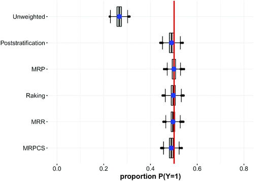
We focus the results section on the bias in the estimation of the proportion of y = 1 and the efficiency of the estimators. In our evaluation of the efficiency of the estimators we compare the Monte-Carlo variances and the mean squared errors (MSEs) of the estimators (see Table 2). In the following sections, we present the results of the simulation study for each scenario separately. For each simulation round, we estimate the proportion for y = 1, and we present the results over all rounds using box plots for the different estimators. The boxes represent the inner 50% of the estimated proportions for y = 1, and the upper and lower bound of the boxes are the 25% and 75% quartiles. The big blue dot within each box denotes the mean proportion of y = 1 over all rounds, and the vertical bars in the box denote the median. The graphs also show the population benchmark which is shown as a red vertical line. Table B.1 in the Appendix shows Cramér’s V statistics for the associations between the inclusion vector and the weighting variables, and for the relations between the weighting variables and the survey variable of interest y for each scenario. The amount of empty cells is provided in Table A.2 and the resulting margins in Table B.2 in the Appendix.

Table 2. Comparisons of Monte-Carlo bias, Monte-Carlo variance (MCvar) and mean squared error (MSE).

Estimator	MCbias	MCvar	MSE
Scenario 1a
Unweighted	−0.2344	0.0002	0.0551
Poststratification	−0.0107	0.0002	0.0003
MRP	−0.0010	0.0001	0.0001
Raking	−0.0035	0.0002	0.0002
MRR	−0.0050	0.0002	0.0002
MRPCS	−0.0121	0.0002	0.0003
Scenario 1b
Unweighted	−0.2344	0.0002	0.0551
Poststratification	−0.0526	0.0002	0.0030
MRP	−0.0579	0.0002	0.0036
Raking	−0.0496	0.0002	0.0027
MRR	−0.0584	0.0002	0.0036
MRPCS	−0.0589	0.0002	0.0037
Scenario 2
Unweighted	−0.4661	0.0000	0.2173
Poststratification	−0.1886	0.0034	0.0390
MRP	−0.0685	0.0084	0.0131
Raking	−0.3206	0.0036	0.1064
MRR	−0.3350	0.0022	0.1144
MRPCS	−0.0719	0.0064	0.0116
Scenario 3
Unweighted	0.1174	0.0004	0.0142
Poststratification	0.0053	0.0006	0.0006
MRP	−0.0105	0.0003	0.0004
Raking	0.0516	0.0004	0.0031
MRR	−0.0104	0.0003	0.0004
MRPCS	−0.0104	0.0003	0.0005

Table A.1. Values for the parameters in the model that generates the survey variable of interest y that is depending on the weighting variables ${\mathbf{x}}_{\mathbf{1}}\dots {\mathbf{x}}_{\mathbf{4}}.$

Parameter	Category	Scenario 1	Scenario 2	Scenario 3
δ		−0.5	−0.5	−12
${\gamma }_{j[i]}^{x_1}$	j = 1	−7	−7	−0.2
	j = 2	0	0	0
	j = 3	−0.2	−0.2	−0.2
	j = 4	0.4	0.4	0.4
	j = 5	7	7	2
${\gamma }_{k[i]}^{x_2}$	k = 1	−7	−7	−1.5
	k = 2	0.4	0.4	0.4
	k = 3	0	0	0
	k = 4	−0.2	−0.2	−0.2
	k = 5	7	7	1.5
${\gamma }_{l[i]}^{x_3}$	l = 1	1.5	1.5	1.5
	l = 2	−0.4	−0.4	−0.4
	l = 3	0	0	0
	l = 4	0.9	0.9	0.9
${\gamma }_{v[i]}^{x_4}$	v = 1	0.1	0.1	–
	v = 2	0.1	0.1	–
	v = 3	0.1	0.1	–
	v = 4	0	0	–
	v = 5	0.1	0.1	–
${\gamma }^{x_5}$	–	–	–	0.8

Table A.2. Values for the parameters in the inclusion model generating the inclusion propensities $\mathbf{\omega }$ that are depending on the weighting variables ${\mathbf{x}}_{\mathbf{1}}\dots {\mathbf{x}}_{\mathbf{4}}.$

Parameter	Category	Scenario 1	Scenario 2	Scenario 3
λ		−1	1e − 07	−14.5
${\xi }_{j[i]}^{x_1}$	j = 1	1	50	−0.1
	j = 2	0	0	0
	j = 3	−0.2	−0.2	−0.2
	j = 4	0.4	0.4	0.4
	j = 5	−1	−50	0.1
${\xi }_{k[i]}^{x_2}$	k = 1	0	0	0
	k = 2	−1	−55	−1e − 07
	k = 3	−1	−55	−1e − 07
	k = 4	−1	−50	−1e − 07
	k = 5	−1	−50	−1e − 07
${\xi }_{l[i]}^{x_3}$	l = 1	0	0	0
	l = 2	0.4	0.4	0.4
	l = 3	0.3	0.3	0.3
	l = 4	0.2	0.2	0.2
${\xi }_{v[i]}^{x_4}$	v = 1	1	50	–
	v = 2	0.1	0.1	–
	v = 3	0	0	–
	v = 4	0.2	0.2	–
	v = 5	−1	−50	–
${\xi }^{x_5}$		–	–	0.9
Weighting cells		500	500	100
Empty cells		217.82	390.97	3.75
		(43.6 %)	(78.2 %)	(3.7 %)

The table includes the numbers of the resulting weighting cells and the amount of empty weighting cells averaged over all simulation rounds.

Table A.3. Values for the parameters in the model that generates ${\mathbf{x}}_{\mathbf{5}}$ that is depending on the weighting variables ${\mathbf{x}}_{\mathbf{1}}\dots {\mathbf{x}}_{\mathbf{3}}.$

Parameter	Category	Scenario 3
a		15
$b_j^{x_1}$	j = 1	−0.2
	j = 2	0
	j = 3	−0.2
	j = 4	0.2
	j = 5	0.3
$b_k^{x_2}$	k = 1	−1
	k = 2	0.4
	k = 3	0
	k = 4	−0.2
	k = 5	1
$b_l^{x_3}$	l = 1	−0.0001
	l = 2	−0.0001
	l = 3	0
	l = 4	0.0001

5.1. Scenario 1a

The results of Scenario 1a (a volunteer sample with moderately skewed inclusion) are presented in Figure 1. The unweighted estimate heavily underestimates the population benchmark, but all the estimates of the weighting procedures are close to the benchmark, and estimates only slightly differed. In this scenario, the inclusion selectivity is not strong, resulting in a low number of empty or sparse cells. Consequently, standard weighting procedures perform as well as complex ones. The MRP approach shows the lowest Monte Carlo variance and MSE.

Figure 1. Scenario 1a—Volunteer sample with moderately skewed inclusion.

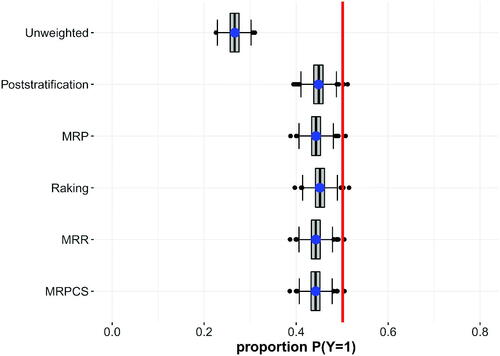
5.2. Scenario 1b

In Scenario 1b, we use the same sample as in Scenario 1a, but we exclude one very influential variable from the weighting and multilevel regression model. As can be seen in Figure 2, the unweighted estimate is heavily biased, and all weighting procedures lead to estimates that come closer to the benchmark. However, none of the standard nor complex procedures lead to an accurate estimate. Also, none of the approaches is able to outperform the others in terms of bias and Monte-Carlo variance. All multilevel approaches show similar MSEs. The findings strengthen the importance of including all characteristics in the weighting procedures that are responsible for the inclusion process. Naturally, in real applications, we do not have benchmarks for all important variables. For this scenario, we also drop the important variable from the multilevel model, but in practice, it might be possible to include such a variable in a multilevel model thereby improving the estimation using complex weighting and estimation procedures. Scenario 3 provides some insight into how including variables in the multilevel model that are not part of the weighting model affects the estimation.

Figure 2. Scenario 1b—Volunteer sample with moderately skewed inclusion and omitted variable in the weighting and multilevel regression models.

5.3. Scenario 2

Figure 3 shows the results for Scenario 2 (a volunteer sample with highly skewed inclusion). The unweighted estimate leads to a highly biased estimate. Standard weighting procedures are able to improve the estimate and poststratification does much better than raking. The MRR approach is not able to outperform standard raking. Two reasons why the MRR procedure is not able to reduce Monte-Carlo bias as compared to standard raking are as follows: first, there are many empty sample cells. As a result, the modified raking approach cannot improve the estimation. Second, in this scenario, the same variables are used in the multilevel and in the weighting models so that the multilevel model cannot achieve an improvement over the standard raking method.

Figure 3. Scenario 2—Volunteer sample with a highly skewed inclusion.

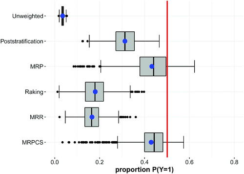
The MRP and MRPCS approaches heavily reduce Monte-Carlo bias as compared to standard raking and even standard poststratification. It is particularly notable, that the estimation using the MRCPS approach lead to a Monte-Carlo bias reduction similar to the MRP approach when using only marginal population information. The Monte-Carlo variances of the MRCPS and MRP approach are similar as well resulting in comparable MSEs. Standard raking and poststratification show lower variances than the MRP and MRCPS approach but higher MSEs due to the higher biases. We assume that the bias reduction of the MRP and MRCPS weighting and complex estimation procedures is due to considering all population cells, even the cells without sample elements, which leads to a stabilized estimation. However, the MRP and the MRPCS approaches also show some larger outliers that are the result of the highly skewed inclusion mechanism and the skewed marginal distributions of this scenario.

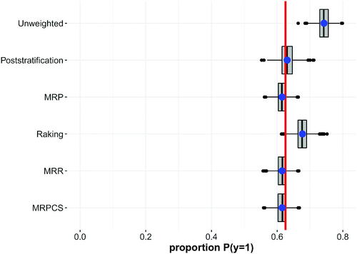
5.4. Scenario 3

The results of Scenario 3 (a volunteer sample with moderate correlations between the weighting variables and the inclusion probability and enriched multilevel regression model) are presented in Figure 4. The unweighted procedure leads to an overestimation of $P(y=1)$ as compared to the benchmark. The standard raking procedure is able to reduce bias but still leads to overestimation. The raking procedure does not include variable x₅ in the weighting model, since it is modeled continuously and is not measured in the survey. However, x₅ can be included in the multilevel model. As a result, the estimates of the MRP approach and the MRR and MRPCS approaches are much closer to the benchmark. For these three approaches, the bias as well as the efficiency are very similar. Surprisingly, the standard poststratification approach is able to reduce bias as compared to the standard raking approach, and yields estimates that are close to the benchmark. The Monte-Carlo variance of the standard poststratification approach, however, is higher than for the multilevel approaches. Although the poststratification procedure does not include x₅, due to the variable generation process based on model 14, some larger correlations exist between variable x₅ and the other weighting variables. It seems that some information on variable x₅ is reproduced over the joint distributions.

Figure 4. Scenario 3—Volunteer sample with highly skewed inclusion. The multilevel model is enriched with information which cannot be included in the weighting model.

6. Summary and conclusion

In this study, we propose two practical approaches to make use of multilevel regression estimations to stabilize weighting procedures when only population margins are available. In a simulation study, we evaluate the performance of our two approaches (MRR and MRPCS) as compared to standard raking and poststratification approaches and multilevel regression and poststratification (MRP). The present study aimed to be highly relevant for social researchers and very applicable, so we only used standard R packages and well established algorithms.

The simulation study shows that for the scenarios with a slightly or moderately skewed inclusion mechanism (Scenario 1a), all standard and complex weighting and estimation approaches work similarly well. In a scenario with highly skewed inclusion propensities (Scenario 2), however, we find big differences between the weighting approaches. MRP and MRPCS are the only approaches that are able to highly reduce Monte-Carlo bias and MRR can only slightly improve the estimation. The inferior performance can be attributed to the high number of empty and sparse cells introduced by the very skewed inclusion mechanism. However, highly skewed inclusion and high numbers of empty cells are typical findings for a volunteer panel for which the MRPCS approach seems especially promising.

Whenever we have a high proportion of empty cells or when we are able to include information on variables of the inclusion model that are not available for the weighting model in the multilevel regression model—e.g., variables that are not captured in the survey—the MRCPS approach reduces bias considerably as compared to standard raking. Unlike the MRPCS approach, the MRR approach cannot deal with empty cells and cannot outperform standard raking when the proportion of empty cells is high. However, with moderate numbers of empty cells, the MRR approach produces comparable results to the MRPCS approach while including fewer estimation steps than the MRPCS approach. The MRR approach consumes less degrees of freedom and is potentially more stable. Both of our proposed approaches, similar to standard raking, depend on the assumption of independent effects of weighting variables on inclusion.

We do not find large differences between the approaches with respect to the omitted variable scenario (Scenario 1b), which means, that no approach is able to compensate for an under specification of the weighting model.

In Scenario 3, we were able to add one relevant variable that could not be considered in the weighting model in the multilevel regression model. We found that all complex weighting approaches to performed equally well in terms of bias and variance, and specifically, that our approaches performed much better than standard raking. In practice, one cannot assume to perfectly know the inclusion model or to have information on all the relevant variables of the inclusion process. Therefore, it is not realistic to rule out bias completely, but the aim should be to reduce bias as much as possible.

In our simulation scenarios, all complex estimation procedures make use of the same set of auxiliary variables. The only difference is that MRP uses joint distributions of the weighing variables, whereas MRR and MRCPS use the margins of the weighting variables. In practice, however, margins usually are available for a higher number of variables than are available for joint distributions, since margins can be gathered from different official data sources. Also, margins usually are aggregated to a lower degree. Thus, often more population information can be utilized working with margins than when working with joint distributions. Thus, it may be worth using complex weighting and estimation methods using a richer set of margins, instead of using a joint distribution of only a few variables. The comparable results for the MRP and MRCPS approaches in our simulation are especially promising.

In most of our scenarios, the multilevel regression model is very simple and only makes use of variables that are part of the weighting model as well. More complex models including a variety of additional hierarchical variables and potentially interactions in the multilevel model are likely to reduce bias even further for all complex models.

The modifications are described with respect to an application of volunteer panels, that do not have design or sampling weights by definition. The MRR and MRCPS approach, as described in the previous sections, can also be applied for probability sampling designs with equal inclusion probabilities, i.e., simple random sampling designs or a so-called self-weighting designs. However, if a more complex sampling design is applied that leads to unequal inclusion probabilities, sampling weights need to be computed. Sampling weights can be included in both of our modifications. For the MRR approach, the sampling weights cannot be directly included in the raking procedure because we apply the raking on the cell level but not individual level. The variables that are used to compute the sampling weights can, however, be included as additional weighting variables. The sampling weights can directly be considered in the multilevel approach, for example, by using the procedures described in Rabe-Hesketh and Skrondal (2006), Pfeffermann et al. (1998) and Asparouhov and Muthen (2006) (see also Gelman (2007) and West and Galecki (2012) for general discussion on this issue). The same procedures can be used to integrate sampling weights in the multilevel model for the MRCPS approach. Furthermore, it is possible to directly include the sampling weights in the estimation of the population sizes ${\widehat{N}}_{\mathit{jklv}}.$ In the estimation procedures by Little and Wu (1991) that we use in our research, this can be done by using the design weighted sample cell frequencies. The sampling weights are then considered in the estimation of the population cell sizes ${\widehat{N}}_{\mathit{jklv}}$ that are used to weight the cell propensities.

Since the approaches we described are applied to non-probabilistic volunteer panels with different degrees of selectivity, we cannot compute variance estimates, e.g., to generate confidence intervals. This is a serious limitation when applying our approach—like many other approaches—to a nonprobabilistic sample. In the case that a comparable probability sample covering the general population of interest is available, variances might be estimated using quasi-randomization, superpopulation or double robust modeling (Elliott and Valliant (2017); Chen, Li, and Wu (2020); for an overview see Cornesse et al. 2020). More research is needed on how to combine these methods with our approaches. When applying our approach on a probabilistic sample, resampling procedures (for a detailed explanation of these procedures see Shao and Tu 1995) like the bootstrap (Efron 1979) can be applied to estimate the variance for our proposed approaches. The variance estimates can be used to compute confidence intervals and perform population inference. As a further consequence of using a non-probabilistic sampling design, the efficiency of the procedures discussed in this paper is evaluated using the Monte-Carlo variance.

Although our results are very promising, further research also should be conducted on how to improve the approaches. For example, in our simulation study, we use rather simple approaches to estimate the cell population sizes in the MRCPS method. In practical applications, the estimation of cell population sizes might be improved by using small area estimation approaches, including more information from additional population information sources from official statistics. Another possibility for improving the estimation could be to smooth the estimated cell population sizes that are obtained via weighted least squares and by using prior information to determine the smooth parameter. The usefulness of such extensions, however, needs to be discussed in further research.

Acknowledgments

The authors thank Matthias Sand, Andreas Fuest and the anonymous reviewer for their helpful comments on this research.

Appendix

A. Parameter values in the simulation study

B. Measures of association of the weighting variables and the survey variable of interest and of the weighting variable and the inclusion vector

Table B.1. Cramér’s V for the association between the weighting variables ${\mathbf{x}}_{\mathbf{1}}\dots {\mathbf{x}}_{\mathbf{4}}$ and the survey variable of interest y, the association between the inclusion vector z and the survey variable of interest y, and the association between the weighting variables and the inclusion vector z.

Association	Scenario 1	Scenario 2	Scenario 3
$C{V}_{\mathbf{x}\mathbf{1},\mathbf{y}}$	0.68	0.68	0.40
$C{V}_{\mathbf{x}\mathbf{2},\mathbf{y}}$	0.59	0.59	0.32
$C{V}_{\mathbf{x}\mathbf{3},\mathbf{y}}$	0.14	0.14	0.23
$C{V}_{\mathbf{x}\mathbf{4},\mathbf{y}}$	0.12	0.12	0.63
$C{V}_{\mathbf{z},\mathbf{y}}$	0.28	0.51	0.18
$C{V}_{\mathbf{x}\mathbf{1},\mathbf{z}}$	0.32	0.51	0.27
$C{V}_{\mathbf{x}\mathbf{2},\mathbf{z}}$	0.33	0.77	0.10
$C{V}_{\mathbf{x}\mathbf{3},\mathbf{z}}$	0.08	0.11	0.09
$C{V}_{\mathbf{x}\mathbf{4},\mathbf{z}}$	0.24	0.36	0.46

Table B.2. Simulated margins for the weighting variables ${\mathbf{x}}_{\mathbf{1}}\dots {\mathbf{x}}_{\mathbf{4}}.$

Variable	Category	Scenario 1	Scenario 2	Scenario 3
${\mathbf{x}}_{\mathbf{1}}$	1	408.21	574.02	98.83
	2	155.44	165.17	175.05
	3	96.20	94.38	99.41
	4	255.65	149.94	240.59
	5	84.50	16.49	386.12
${\mathbf{x}}_{\mathbf{2}}$	1	482.35	853.54	224.57
	2	216.50	62.50	252.55
	3	175.31	25.46	232.10
	4	84.08	46.64	170.13
	5	41.76	11.86	120.66
${\mathbf{x}}_{\mathbf{3}}$	1	266.09	317.98	210.13
	2	288.97	268.90	267.14
	3	246.11	229.88	262.46
	4	198.82	183.24	260.27
${\mathbf{x}}_{\mathbf{4}}$	1	411.71	519.74
	2	229.30	219.88
	3	199.71	168.47
	4	128.58	80.58
	5	30.70	11.33

References

- Asparouhov, T., and B. Muthen. 2006. Multilevel modeling of complex survey data. ASA section on Survey Research Methods. Proceedings of the Joint Statistical Meetings; Seattle, WA. August 2006, 2718–26.
- Barthélemy, J., and T. Suesse. 2018. mipfp: An R package for multidimensional array fitting and simulating multivariate Bernoulli distributions. Journal of Statistical Software 86 (Code Snippet 2):1–20. doi: 10.18637/jss.v086.c02.
- Bates, D., M. Mächler, B. Bolker, and S. Walker. 2015. Fitting linear mixed-effects models using lme4. Journal of Statistical Software 67 (1):1–48. doi: 10.18637/jss.v067.i01.
- Burgard, J. P. 2015. Evaluation of small area techniques for applications in official statistics. Doctoral thesis, Universität Trier.
- Callegaro, M., K. L. Manfreda, and V. Vehovar. 2015. Web survey methodology. London: SAGE.
- Chen, Y., P. Li, and C. Wu. 2020. Doubly robust inference with nonprobability survey samples. Journal of the American Statistical Association 115 (532):2011–21. doi: 10.1080/01621459.2019.1677241.
- Cornesse, C., A. G. Blom, D. Dutwin, J. A. Krosnick, E. D. De Leeuw, S. Legleye, J. Pasek, D. Pennay, B. Phillips, J. W. Sakshaug, et al. 2020. A review of conceptual approaches and empirical evidence on probability and nonprobability sample survey research. Journal of Survey Statistics and Methodology 8 (1):4–36. doi: 10.1093/jssam/smz041.
- Deming, W. E., and F. F. Stephan. 1940. On a least squares adjustment of a sampled frequency table when the expected marginal totals are known. The Annals of Mathematical Statistics 11 (4):427–44. doi: 10.1214/aoms/1177731829.
- Efron, B. 1979. Bootstrap methods: Another look at the jackknife. The Annals of Statistics 7 (1):1–26. doi: 10.1214/aos/1176344552.
- Elliott, M. R., and R. Valliant. 2017. Inference for nonprobability samples. Statistical Science 32 (2):249–64. doi: 10.1214/16-STS598.
- Enderle, T., R. Münnich, and C. Bruch. 2013. On the impact of response patterns on survey estimates from access panels. Survey Research Methods 7 (2):91–101.
- Gelman, A. 2007. Struggles with survey weighting and regression modeling. Statistical Science 22 (2):153–64. doi: 10.1214/088342306000000691.
- Gelman, A., and J. B. Carlin. 2000. Poststratification and weighting adjustments. In Survey nonresponse, ed. R. M. groves, D. A. Dillman, J. L. Eltinge and R. L. A. Little, 289–302. New York: John Wiley & Sons, Inc.
- Gelman, A., and J. Hill. 2006. Data analysis using regression and multilevel/hierarchical models. Cambridge, UK: Cambridge University Press.
- Gelman, A., and T. C. Little. 1997. Poststratification into many categories using hierarchical logistic regression. Survey Methodology 23 (2):127–35.
- Gelman, A., J. B. Carlin, H. S. Stern, D. B. Dunson, A. Vehtari, and D. B. Rubin. 2013. Bayesian data analysis. New York: Chapman and Hall/CRC.
- Genz, A., F. Bretz, T. Miwa, X. Mi, F. Leisch, F. Scheipl, and T. Hothorn. 2019. mvtnorm: Multivariate normal and t distributions. R package version 1.0-11.
- Ghitza, Y., and A. Gelman. 2013. Deep interactions with MRP: Election turnout and voting patterns among small electoral subgroups. American Journal of Political Science 57 (3):762–76. doi: 10.1111/ajps.12004.
- Ghosh, M., and J. Rao. 1994. Small area estimation: An appraisal. Statistical Science 9 (1):55–76. doi: 10.1214/ss/1177010647.
- Ireland, C. T., and S. Kullback. 1968. Contingency tables with given marginals. Biometrika 55 (1):179–88. doi: 10.1093/biomet/55.1.179.
- Kalton, G., and I. Flores-Cervantes. 2003. Weighting methods. Journal of Official Statistics 19 (2):81–97.
- Kastellec, J. P., J. R. Lax, M. Malecki, and J. H. Phillips. 2015. Polarizing the electoral connection: Partisan representation in supreme court confirmation politics. The Journal of Politics 77 (3):787–804. doi: 10.1086/681261.
- Leemann, L., and F. Wasserfallen. 2017. Extending the use and prediction precision of subnational public opinion estimation. American Journal of Political Science 61 (4):1003–22. doi: 10.1111/ajps.12319.
- Little, R. J. A. 1993. Post-stratification: A modeler’s perspective. Journal of the American Statistical Association 88 (423):1001–12. doi: 10.1080/01621459.1993.10476368.
- Little, R. J., and M.-M. Wu. 1991. Models for contingency tables with known margins when target and sampled populations differ. Journal of the American Statistical Association 86 (413):87–95. doi: 10.1080/01621459.1991.10475007.
- Little, R., and S. L. Vartivarian. 2005. Does weighting for nonresponse increase the variance of survey means? Survey Methodology 31:161–8.
- Park, D. K., A. Gelman, and J. Bafumi. 2004. Bayesian multilevel estimation with poststratification: State-level estimates from national polls. Political Analysis 12 (4):375–85. doi: 10.1093/pan/mph024.
- Pasek, J. 2018. anesrake: ANES Raking Implementation. R package version 0.80.
- Pfeffermann, D., C. J. Skinner, D. J. Holmes, H. Goldstein, and J. Rasbash. 1998. Weighting for unequal selection probabilities in multilevel models. Journal of the Royal Statistical Society: Series B (Statistical Methodology) 60 (1):23–40. doi: 10.1111/1467-9868.00106.
- R Core Team. 2017. R: A language and environment for statistical computing. Vienna, Austria: R Foundation for Statistical Computing.
- Rabe-Hesketh, S., and A. Skrondal. 2006. Multilevel modelling of complex survey data. Journal of the Royal Statistical Society: Series A (Statistics in Society) 169 (4):805–27. doi: 10.1111/j.1467-985X.2006.00426.x.
- Shao, J., and D. Tu. 1995. The jackknife and bootstrap. New York: Springer.
- Si, Y., and P. Zhou. 2021. Bayes-raking: Bayesian finite population inference with known margins. Journal of Survey Statistics and Methodology 9 (4):833–55. doi: 10.1093/jssam/smaa008.
- Statisticat and LLC. 2018. Laplacesdemon: Complete environment for Bayesian inference. R package version 16.1.1.
- Wang, W., D. Rothschild, S. Goel, and A. Gelman. 2015. Forecasting elections with non-representative polls. International Journal of Forecasting 31 (3):980–91. doi: 10.1016/j.ijforecast.2014.06.001.
- West, B. T., and A. T. Galecki. 2012. An overview of current software procedures for fitting linear mixed models. The American Statistician 65 (4):274–82. doi: 10.1198/tas.2011.11077.