Variance stabilizing filters^#

Abstract

In this paper new filters for removing unspecified form of heteroscedasticity are proposed. The filters build on the assumption that the variance of a pre-whitened time series can be viewed as a latent stochastic process by its own. This makes the filters flexible and useful in many situations. A simulation study shows that removing heteroscedasticity before fitting a model leads to efficiency gains and bias reductions when estimating the parameters of ARMA models. A real data study shows that pre-filtering can increase the forecasting precision of quarterly US GDP growth.

Keywords:

• Time series
• heteroscedasticity filters
• simulation studies
• US GDP
• Kalman filter

JEL classification:

• C13
• C15

1. Introduction

Economic and financial variables often behave in a non-stationary way (Granger 1966). They might suffer from seasonality, unit roots, non-linearity and heteroscedasticity that must be dealt with before, or at the same time as estimating a model. The first difference of the logarithm (diff log) of a de-seasonalized series is often used as a standard filter to transform a non-stationary time series into a stationary one (Box and Jenkins 1976). Most of the times this is enough for the series to pass unit root tests, but they might still be heteroscedastic – a feature that is frequently neglected among practitioners. This is somewhat surprising since it is well known that ordinary least squares (OLS) estimates are inefficient and no longer best linear unbiased estimators (BLUE) in the presence of heteroscedasticity. This paper offers a way to address this issue by introducing new filters that easily and effectively remove heteroscedasticity of unspecified form.

There are not many ways of removing heteroscedasticity mentioned in the literature. One way is to use a Box-Cox transformation (Box and Cox 1964) which include the logarithmic and square root transformations as special cases. However, the Box-Cox transformations only work well when the functional form of the variance does not change throughout the series, rarely a realistic assumption in practice. Stockhammar and Öller (2012) developed a way to remove unspecified form of heteroscedasticity by estimating the standard deviations in a moving lag-window and using a similar idea as in generalized least squares (GLS) to scale the series.

In this paper, new variance stabilizing filters are suggested that improve on the filter suggested by Stockhammar and Öller (2012) in a number of ways. In addition, the properties of the new filters are investigated through both a real data exercise and a simulation study. It is shown that the proposed filters remove different types of heteroscedasticity without changing the autocorrelation structure or other properties of the series. The simulation study shows that stabilizing the series leads to more efficient estimates of the ARMA parameters. The filtering approach proposed in this paper outperforms estimated GARCH models (Bollerslev 1986) when the variance follows three different regimes and, interestingly, compare well even for simulated ARMA-GARCH processes. Furthermore, it is shown that the filters does not color white noise and that existing autocorrelation structures are preserved.

In a real data exercise the heteroscedastic and non-normal quarterly diff log US GDP is filtered. After filtering the series is homoscedastic and closer to normal. Also, a pseudo-out-of-sample forecast competition shows that forecast precision is elevated using the filtering approach.

The coming section describes the methodological framework for the filtering and the simulations. Section 3 contains a summary of the results and Section 4 concludes.

2. Methodology

In this section, the methodology is outlined. Specifically, the filtering approaches are explained in detail, the biasedness of autoregressive parameter estimates is discussed and the simulation models and the evaluation procedures are described.

2.1. The filters

2.1.1. The original filter

In the original filter suggested by Stockhammar and Öller (2012) the idea is to divide the time series by a smoothed moving standard deviation observed in the sample. The first step is to make the series stationary by a suitable transformation, the standard deviations are then calculated in a moving lag-window and are further smoothed using a HP-trend, (Hodrick and Prescott 1997). The next step is to divide the mean-stationary and mean-corrected series ($z_t)$by the HP-trend to obtain a homoscedastic time series. Finally, the time series is scaled back to have the same mean and variance as the original series.

The filter can be expressed in the following way: (1) $$\begin{array}{c}{\tilde{y}}_t=s_y\left[\frac{z_t}{H{P}^{(\lambda )}\left\{\sqrt{\sum _{\tau =t-\nu }^{t+\nu }{z}_{\tau }^2/2\nu }\right\}}\right]+\overline{y},\end{array}$$(1) where ${\tilde{y}}_t$ is the filtered series, $\overline{y}$ and s_y are the mean and standard deviation of the series to be filtered respectively. 2ν + 1 denotes the length of the lag-window and HP^(λ) denotes the Hodrick and Prescott filter where λ controls the degree of smoothing. The suggested value for quarterly data λ = 1600 is used in this study. The filter offers a fast and simple way to remove heteroscedasticity of unspecified form. However, because of the smoothed standard deviations, the heteroscedasticity filtering is not efficient in presence of rapidly changing volatility.

2.1.2. Modifications of the original filter

The modified filters suggested in this subsection all use (in contrast to the original filter) pre-whitening before the smoothed standard deviations are calculated. The reason is that even a mean-stationary process which deviates from zero will only slowly return to steady-state generating a cluster where the squared deviations from zero are high. If no pre-whitening of the series is conducted in beforehand these deviations will be interpreted as an increased variance by the filters. This implies that the variance is scaled in a time window where it actually behaves homoscedastic. On the other hand, if the model is pre-whitened before, the effect from the autocorrelation is accounted for and what is left as increased variance in the pre-whitened series would be isolated to the underlying heteroscedasticity.

Another potential issue with the original approach is the use of the often criticized (see e.g. Hamilton (2017)) HP-filter where the user subjectively chooses a level for the degree of smoothing, λ. A more flexible way is to estimate the degree of smoothing automatically from a time series $x_t$ using the Kalman filter. For this purpose, the local linear trend model (LLTM) is used (see e.g. Durbin and Koopman (2012)).

The LLTM has the following state-space representation: (2) $${\mathit{x}}_{\mathit{t}}={\mathit{\alpha }}_{\mathit{t}}+{\mathit{ϵ}}_{\mathit{t}}, {\mathit{ϵ}}_{\mathit{t}}\sim \mathit{N}(0,{\mathit{\sigma }}_{\mathit{ϵ}}^2)$$(2) (3) $${\mathit{\alpha }}_{\mathit{t}+1}={\mathit{\alpha }}_{\mathit{t}}+{\mathit{\beta }}_{\mathit{t}}+{\mathit{\eta }}_{\mathit{t}}, {\mathit{\eta }}_{\mathit{t}}\sim \mathit{N}(0,{\mathit{\sigma }}_{\mathit{\eta }}^2)$$(3) (4) $${\beta }_{\mathit{t}+1}={\beta }_{\mathit{t}}+{\xi }_{\mathit{t}},{\xi }_t\sim N(0,{\sigma }_{\xi }^2)$$(4) where the error terms, ${\mathit{ϵ}}_{\mathit{t}}, {\mathit{\eta }}_{\mathit{t}}$ and ${\mathit{\xi }}_{\mathit{t}}$ are independent white noise processes. ${\mathit{\alpha }}_{\mathit{t}}$ and ${\mathit{\beta }}_{\mathit{t}}$ denote the “local level” and the “local linear trend” respectively and ${\mathit{x}}_{\mathit{t}}$ is the observed time series. Ledolter (2008) shows in a simulation study that this type of smoothing works well compared to for example local polynomial regressions where a moving lag window is used. To achieve a smooth trend it is possible to restrict the variance of the second equation to zero, which is sometimes referred to as “the smooth trend model” (STM). The same effect can be achieved by replacing Equations (3)(3) $${\mathit{\alpha }}_{\mathit{t}+1}={\mathit{\alpha }}_{\mathit{t}}+{\mathit{\beta }}_{\mathit{t}}+{\mathit{\eta }}_{\mathit{t}}, {\mathit{\eta }}_{\mathit{t}}\sim \mathit{N}(0,{\mathit{\sigma }}_{\mathit{\eta }}^2)$$(3) and (4)(4) $${\beta }_{\mathit{t}+1}={\beta }_{\mathit{t}}+{\xi }_{\mathit{t}},{\xi }_t\sim N(0,{\sigma }_{\xi }^2)$$(4) by ${\Delta }^2{\mathit{\alpha }}_{\mathit{t}+1}={\mathit{\eta }}_{\mathit{t}}\iff {\mathit{\alpha }}_{\mathit{t}+1}=2{\mathit{\alpha }}_{\mathit{t}}-{\mathit{\alpha }}_{\mathit{t}-1}+{\mathit{\eta }}_{\mathit{t}},$in this case we have an integrated random walk (IRW) which together with the extension ${\Delta }^r{\mathit{\alpha }}_{\mathit{t}+1}={\mathit{\eta }}_{\mathit{t}}, \mathit{r}>2$ has been recommended for modeling trends in state space models (see Durbin and Koopman (2012) and Young et al. (1991)). When the smoothing parameter of the HP-filter λ = ${\sigma }_{\mathit{\eta }}^2/{\sigma }_{\mathit{ϵ}}^2$, it is equivalent to the IRW. For completeness, both the case with ${\mathit{\sigma }}_{\mathit{\eta }}^2$=0 and the unrestricted case will be investigated in the coming analysis.

In addition to the original filter of Stockhammar and Öller (2012), we consider three modified heteroscedasticity filters which all build on the pre-whitened, mean-corrected and possibly heteroscedastic series, ${\mathit{z}}_{\mathit{t}}$, which absolute value we denote by ${\mathit{x}}_{\mathit{t}}$.

• “HP variance filter” uses the HP-filter on ${\mathit{x}}_{\mathit{t}}$to estimate the standard deviation.

• “LLTM variance filter” uses the LLTM on ${\mathit{x}}_{\mathit{t}}$ to estimate the standard deviation.

• “STM variance filter” uses the STM on ${\mathit{x}}_{\mathit{t}}$ to estimate the standard deviation.

All filters are likely to produce a good degree of smoothing if the volatility smoothly evolves over time. However, if there are jumps or more rapid changes in the variance process, then the LLTM is expected to adjust faster than the others since it does not force smoothness on the states to the same extent.

The filtered version of the original series is obtained by dividing the mean-corrected series by the moving standard deviation. The series is then scaled back to have the same overall variance and mean as $y_t$. We define $y_t^{*}=\frac{y_t-\overline{y}}{{\widehat{\sigma }}_t^e}$, where ${\widehat{\sigma }}_t^e$ is the low-frequency evolution of the standard deviation estimated by inserting $x_t$ into (2)–(4). The filtered series is then given by: (5) $${\tilde{y}}_t=s_y\left[\frac{y_t^{\mathit{*}}-\overline{y^{\mathit{*}}}}{s_{\mathit{*}}}\right]+\overline{y}$$(5) where$\mathit{ }\overline{y}$ and $s_y$ are the sample mean and standard deviation of $y_t$ respectively, and $\overline{y^{*}}$ and $s_{*}$ denote the mean and standard deviation of $y_t^{*}$. If we want to recover the original series we may reverse the filter according to: (6) $$y_t={\widehat{\sigma }}_t^e\left[\frac{s_{\mathit{*}}}{s_y}\left({\tilde{y}}_t-\overline{y}\right)+\overline{y^{\mathit{*}}}\mathit{ }\right]+\overline{y}$$(6) where we already have the information needed to go back from (5). The same approach can be used to transfer back fitted values with confidence intervals (as is later shown in the real data exercise). In the case of forecasting and forecast intervals, we can proceed in a similar way. The only difference is that we do not have access to ${\widehat{\sigma }}_{t+h}^e$, i.e. future values of the low-frequency volatility, but it might be approximated by simply rolling the Kalman filter forward.

2.2. Biasedness of OLS

It is known that the OLS and ML estimates of AR-coefficients are consistent but biased (e.g. Hamilton 1994). When conditioning an AR(1)-process on the whole realization of the series, the bias of the estimator is given by: (7) $$E\left[\widehat{\varphi }|y_1,y_2,\dots ,y_n\right]-\varphi =\sum _{t=2}^{n}E\left[\frac{y_{t-1}}{\sum _{t=2}^n{y}_{t-1}^2}{ϵ}_t|y_1,y_2,\dots ,y_n\right]$$(7) where $\varphi$ is the AR(1) parameter and ${ϵ}_t$ is the error term. The bias of the estimator (7) is non-zero. We may note that $\mathit{E}\left[{\mathit{y}}_{\mathit{t}-1}{\mathit{ϵ}}_{\mathit{t}}\right|{\mathit{y}}_1,{\mathit{y}}_2,\dots ,{\mathit{y}}_{\mathit{n}}]$ = 0, but the errors are not uncorrelated with the sum in the denominator. Intuitively this can be seen since a high absolute value of the error term today increases the value of ${\mathit{y}}^2$ in future periods, thus the bias will be negative for ϕ > 0 and positive for ϕ < 0. This means that the OLS (as well as the conditional likelihood) estimates will be drawn toward zero, but that the bias decrease with the sample size. See e.g. Rai et al. (1995) for a discussion and a simulation study of the bias in small samples. Later, in the results, we will see that filtering has a dampening effect on the attenuation bias in the presence of heteroscedasticity.

2.3. The simulated processes

In this section, 10 000 realizations are simulated from four different processes to evaluate the influence of the above filtering procedures. All of the series are chosen to be of length 200, the approximate length of many quarterly macroeconomic time series. For the ARMA model, two different sample sizes are investigated. The first two series are simulations from homoscedastic white noise- and ARMA processes in order to see that the filters do not change structures intended to be preserved. In addition, two heteroscedastic processes are simulated to see whether the filters can achieve homoscedasticity.

In the first heteroscedastic process, the error term follows the frequently used GARCH structure (Bollerslev 1986) and in the second the variance evolves according to three different volatility periods. In both cases, the mean-process will be ARMA(1,1) with arbitrarily chosen parameters, ϕ = 0.7 and θ = 0.5.¹

That is, we simulate from the ARMA-GARCH process given by: (8) $$y_t=0.7y_{t-1}+\mathit{ }{a}_t+{0.5a}_{t-1},\mathit{ }{a}_t={\sigma }_t{ϵ}_t,\mathit{ }{\sigma }_t^2=1+0.12a_{t-1}+0.82{\sigma }_{t-1}^2$$(8) which clearly satisfies the conditions for the variance to be positive and finite, see e.g. Tsay (2010).

In the second heteroscedastic process (“the switching variance model”) the volatility changes according to pre-specified regimes: $$y_t=0.7y_{t-1}+a_t+{0.5a}_{t-1},\mathit{ }{\mathit{ }a}_t\sim N(0,{\sigma }_t^2),$$ (9) $${\sigma }_t^2=4\times {\mathbb{I}}_{\left(\mathrm{0,40}\right]}\left(t\right)+1\times {\mathbb{I}}_{\left[\mathrm{41,140}\right]}\left(t\right)+16\times {\mathbb{I}}_{\left[\mathrm{141,200}\right]}\left(t\right)$$(9) where $\mathbb{I}$ denotes an indicator variable which divides the series into three arbitrary chosen volatility periods of different length. It can be seen as a threshold model with three distinct regimes and with time as the regime-controlling variable.

2.4. Evaluation procedure

One of the most important parts of filtering is that it does what it is intended to do without changing other properties of the time series. This is investigated in two ways; first, the filters are tested on simulated white noise to see whether the first four moments remain unchanged. This is done by calculating the means and (empirical) standard deviations for the simulated moments. The series are also tested for non-normality using the Jarque-Bera test (Jarque and Bera 1980) and for autocorrelation using the Ljung-Box test (Ljung and Box 1978) to make sure that no spurious autocorrelations are imposed.

This is complemented using the probability integral transform (PIT), see e.g. Diebold et al. (1998), which is defined as: (10) $$\begin{array}{c}{v}_t={\int }_{-\mathit{\infty }}^{y_t}{p}_t\left(u\right)du\end{array}$$(10) where ${\mathit{y}}_{\mathit{t}}\mathit{ }$are realizations of a time series and ${\mathit{p}}_{\mathit{t}}(\mathit{u})$ is the assumed density. If ${\mathit{p}}_{\mathit{t}}(\mathit{u})$ is the true density we have${\mathit{v}}_{\mathit{t}}\sim \mathit{U}(0, 1)$, so deviations from the uniform distribution indicate model misspecification. For the PIT exercises, only one simulated time series of length 10 000 is used.

The outlined tests will be made on the simulated series as well as when the series are run through each of the filters. It is also investigated whether it preserves existing autocorrelations structures in simulated (homoscedastic) ARMA-processes.

After investigations on homoscedastic data, we study whether the filters offer improvements compared to unfiltered ARMA- and the less parsimonious ARMA-GARCH models on heteroscedastic data. The focus is on the efficiency for estimating the ARMA parameters and whether there is remaining heteroscedasticity in the model residuals. We make use of the ARCH-LM test (Engle 1982) to test for constancy of the residual variance and an F-test for checking whether the variance is stable in sub-periods of the series (see e.g. Durbin and Koopman (2012), p. 39). Also the probability integral transform is used to graphically see how well the residuals fit a normal distribution.

When evaluating the filter on the log diff US GDP the above tests are complemented with the Ljung-Box test on the squared residuals when testing for heteroscedasticity. The normality tests are complemented with the (Royston 1982) extension of the Shapiro-Wilk test (Shapiro and Wilk 1965) and the Kolmogorov-Smirnov test (Smirnov 1948).

3. Results

This section summarizes the results from the simulation studies and the forecasting competitions of the heteroscedastic US GDP.

3.1. Simulation studies

3.1.1. White noise

Table 1 shows how the filters affect the properties of white noise in terms of the first four moments, the Jarque-Bera test for normality and the Ljung-Box test for autocorrelation. It is of highest importance that the filters do not impose false autocorrelation structures and/or cause other spurious patterns in the time series.

Table 1. Summary of simulation results for white noise processes.

Type	White Noise	S&Ö	HP	LLTM	STM
Mean	0.000 (0.071)	0.000 (0.071)	0.000 (0.071)	0.000 (0.071)	0.000 (0.071)
Variance	0.999 (0.100)	0.999 (0.100)	0.999 (0.100)	0.999 (0.100)	0.999 (0.100)
Skewness	0.003 (0.170)	0.001 (0.136)	0.001 (0.156)	0.001 (0.167)	0.001 (0.168)
Kurtosis	2.942 (0.330)	2.655 (0.230)	2.776 (0.296)	2.904 (0.329)	2.923 (0.330)
Jarque-Bera	465	101	219	394	422
Ljung-Box, 1 lags	534	424	649	553	548
Ljung-Box, 6 lags	529	343	475	500	517
Ljung-Box, 12 lags	606	380	513	580	582
Ljung-Box, 24 lags	675	554	656	644	643

Note: The HP-filter is used with λ = 1600 to smooth the absolute value of the pre-whitened series, while LLTM uses the local linear trend model and STM the smooth trend model. S&Ö corresponds to the filter of Stockhammar and Öller (2012). The top part of the table presents the means of the empirical moments with standard deviations in parentheses and the bottom part shows the number of rejections at the 5%-level out of the 10 000 draws.

There is no major distortion of the true white noise process and the first two moments are identical for all filters by construction. The filtered series remain symmetric, however, the kurtosis is somewhat distorted for both the Stockhammar and Öller filter and the HP variance filter (but it is still within two standard deviations from 3).

The lower part of Table 1 shows that normality is rejected less often for the filtered series. The distortion of the normality tests is again worst for the Stockhammar and Öller- and the HP variance filters even though there is a tendency for all filters to make the data more normal. This could be due to that the filters fade out outliers since these are interpreted as increased variance. The distortion of normality is, however, hard to detect from the PITs in Figure A1 in Appendix A.

When it comes to the autocorrelation tests the rejection rates look similar to those of the true processes for all but the filter of Stockhammar and Öller. This means that the newly proposed filters do not impose false autocorrelation structures.

3.1.2. ARMA processes

Table 2 shows a summary of the simulation study where 10 000 ARMA processes were simulated for two different time series lengths. Each of these series were filtered and the parameters were estimated using an ARMA model.

Table 2. Summary of simulation results for ARMA processes.

	Type	Unfiltered	S&Ö	HP	LLTM	STM
n =200 ϕ = 0.7	Mean	0.692 (0.058)	0.631 (0.066)	0.693 (0.060)	0.692 (0.058)	0.692 (0.058)
θ = 0.5	Mean	0.505 (0.071)	0.500 (0.080)	0.505 (0.073)	0.505 (0.071)	0.505 (0.071)
n = 80 ϕ = 0.7	Mean	0.681 (0.095)	0.630 (0.108)	0.681 (0.098)	0.681 (0.097)	0.681 (0.096)
θ = 0.5	Mean	0.514 (0.121)	0.509 (0.135)	0.512 (0.125)	0.514 (0.123)	0.513 (0.122)

Note: Estimates of the means and empirical std. deviations (in parentheses) of the ARMA parameters. The HP-filter is used with λ = 1600 to smooth the absolute value of the pre-whitened series, while LLTM uses the local linear trend model and STM the smooth trend model. S&Ö corresponds to the filter of Stockhammar and Öller (2012).

Contrary to the Stockhammar and Öller filter, the modified filters seem to preserve the underlying autocorrelation structure. In addition, the LLTM- and the STM filters have equally low standard errors as the true unfiltered ARMA for the sample size of 200. For the sample size of 80, there are only slight differences. The PITs look close to identical to those in the white noise case and are therefore not included (but are available from the authors upon request).

3.1.3. ARMA-GARCH processes

Table 3 shows the results from 10000 simulated series from the ARMA-GARCH(1,1)(1) model, see Equation (8)(8) $$y_t=0.7y_{t-1}+\mathit{ }{a}_t+{0.5a}_{t-1},\mathit{ }{a}_t={\sigma }_t{ϵ}_t,\mathit{ }{\sigma }_t^2=1+0.12a_{t-1}+0.82{\sigma }_{t-1}^2$$(8) .

Table 3. Summary of simulation results for ARMA-GARCH processes.

Model/Parameter	Unfiltered	S&Ö	HP	LLTM	STM	GARCH(1,1)
ϕ1 = 0.7	0.689 (0.066)	0.629 (0.069)	0.694 (0.062)	0.695 (0.062)	0.692 (0.063)	0.695 (0.061)
θ1 = 0.5	0.505 (0.082)	0.504 (0.078)	0.503 (0.077)	0.506 (0.077)	0.506 (0.077)	0.501 (0.076)
ARCH-LM, p = 1	3813	1839	677	664	1205	71
ARCH-LM, p = 3	5266	2165	894	703	1460	286
ARCH-LM, p = 6	5559	2166	1424	777	1425	364
ARCH-LM, p = 12	5255	2091	2345	837	1212	430
ARCH-LM, p = 24	4517	1866	3063	1009	1064	512
F-test	6300	4552	53	161	455	3595

Note: Estimates of the means and empirical std. deviations (in parentheses) of the ARMA parameters. The HP-filter is used with λ = 1600 to smooth the absolute value of the pre-whitened series, while LLTM uses the local linear trend model and STM the smooth trend model. S&Ö corresponds to the filter of Stockhammar and Öller (2012). Bottom part contains the number of rejections out of the 10 000 draws for the respective test where p denotes the lag length of the ARCH-LM test.

As judged by the ARCH-LM tests it appears that when the time series follow a GARCH process the filters are not able to fully clean out the heteroscedasticity. A plausible reason for this is that the volatility is switching too rapidly such that the smoothing filters do not react fast enough. However, the LLTM filter does a decent job and the null hypothesis of homoscedasticity is typically rejected in less than 10% of the simulations. Looking at the F-tests for constancy of the variance over sub-periods we can see that the three modified filters effectively remove this type of heteroscedasticity. This is not the case for the other approaches, not even for the GARCH model which generated the data.

Looking at the parameter estimates we can see that, compared to the standard ARMA model, the filters reduce the bias of the AR-coefficient in all cases except for the filter of Stockhammar and Öller. The moving average estimates are close to the true in all cases. In addition, all specifications except for the original filter produce smaller standard errors for the parameters compared to the unfiltered series.

Figure A1 in Appendix A shows that the residuals of the true model, the Stockhammar and Öller- and the STM filter are close to normally distributed whereas the errors from the unfiltered approach are leptokurtic. The residuals from the HP- and LLTM filters seem to be slightly platykurtic.

3.1.4. Switching variance model

In Table 4 the simulated processes are created with three different variance regimes. In the first regime (observations 1–40), σ = 2, in the second regime (41–140) σ = 1 and in the third regime (141–200) σ = 4, see Equation (9)(9) $${\sigma }_t^2=4\times {\mathbb{I}}_{\left(\mathrm{0,40}\right]}\left(t\right)+1\times {\mathbb{I}}_{\left[\mathrm{41,140}\right]}\left(t\right)+16\times {\mathbb{I}}_{\left[\mathrm{141,200}\right]}\left(t\right)$$(9) .

Table 4. Summary of simulation results for switching variance processes.

Model/Parameter	Unfiltered		S&Ö	HP	LLTM	STM	GARCH(1,1)
ϕ1 = 0.7	0.683 (0.084)		0.636 (0.071)	0.698 (0.066)	0.699 (0.066)	0.696 (0.067)	0.693 (0.071)
θ1 = 0.5	0.496 (0.106)		0.482 (0.086)	0.487 (0.079)	0.491 (0.078)	0.485 (0.081)	0.489 (0.090)
ARCH-LM, p = 1	6984		1665	515	544	921	714
ARCH-LM, p = 3	8928		1808	586	578	1010	890
ARCH-LM, p = 6	9420		1783	781	607	953	871
ARCH-LM, p = 12	9591		1644	1168	606	759	793
ARCH-LM, p = 24	9618		1489	1594	629	587	637
F-test	10000		4645	868	1575	2851	9971

Note: Estimates of the means and empirical std. deviations (in parentheses) of the ARMA parameters from the switching variance model. The HP-filter is used with λ = 1600 to smooth the absolute value of the pre-whitened series, while LLTM uses the local linear trend model and STM the smooth trend model. S&Ö corresponds to the filter of Stockhammar and Öller (2012). The bottom part of the table contains the number of rejections out of the 10 000 simulations for each test where p denotes the lag length of the ARCH-LM test.

It is clear that also under this form of heteroscedasticity the modified filtering approaches offers both bias reductions and efficiency gains compared to regular ARMA models. The filtered models also yield lower standard deviations of the empirical distribution (and smaller bias) than the GARCH model, which in turn is still to prefer compared to the ARMA.²

The LLTM filter succeeds best in eliminating ARCH effects while the HP variance filter most efficiently even out the variance according to the F-test. The original filter does not perform particularly well and the GARCH model works fairly well for ARCH effects but not according to the F-test.

3.1.5. Bias reduction

According to the simulations, the filtering appears to give less biased estimates for the AR-parameters than the non-filtered approach for heteroscedastic data. This phenomenon is further investigated in this section. In Section 2 it was shown that the estimates of autoregressive components are biased toward zero. The size of the bias is determined by the correlation between the error term and the sum of squares, which violates the least squares assumption of strict exogeneity.

The switching volatility model from (9) will be used to evaluate the effect of filtering on the estimation bias. 10 000 time series are simulated for a grid of sample sizes ranging from 25 to 500. For each sample size, the empirical means and standard deviations of the estimated AR coefficients are calculated for the unfiltered series and the ones filtered using the LLTM. The results are illustrated in Figure 1.

Figure 1. Average point estimates (left panel) and empirical standard deviations (right panel) for ϕ in the 10 000 draws. The dashed blue lines show the results from the LLTM filtered series and the solid black lines from the unfiltered ARMA.

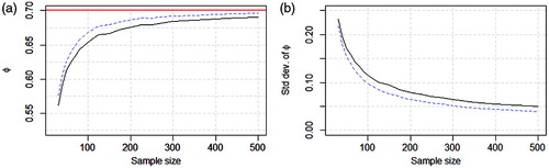
It is clear that the LLTM approach (represented by the blue dashed line) is both less biased and has smaller standard errors than the unfiltered (solid black line). This is true for all sample sizes investigated even though the numerical differences get smaller as the sample size increases.

3.2. A real data study

In this section, the filtering approach is applied to the heteroscedastic quarterly diff log US GDP series 1947Q2-2017Q1. No matter which filtering method used, the heteroscedasticity is removed after the filtering, see Table B1 in Appendix B. It is investigated how the filtering affect the statistical properties as well as the forecast accuracy when modeling the series.

A benefit of being able to recover the original scale from the filtered series is illustrated by calculating 95% confidence intervals for the filtered series and transfer them back to the original scale. Figure 2 shows how the properties of the intervals are improved.

Figure 2. Diff log US GDP (red solid), fitted values of ARMA(2,1) (black solid) and 95% confidence intervals (blue dashed). Unfiltered series (left panel) and LLTM-filtered series (right panel).

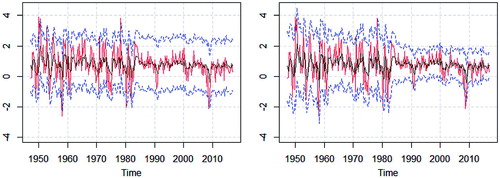
The filtering approach lets the width of the confidence bands to vary over time which improves the coverage rates in both the first and second half of the sample. In this example with an intended coverage rate of 95%, the unfiltered approach yields a coverage of 93% for the full sample while the filtered approach yields a 95% coverage. If the full sample is divided into two halves the regular approach yields 87% and 99% coverage respectively for the first and second half, while the filtering approach generates a 95% and 96% coverage.

For the data study, we first fit the best ARIMA model which is identified by minimizing the AIC and BIC while the conditions that we have no unit root and no remaining autocorrelation in the residuals hold. This approach showed that the best fit was accomplished by an AR(1) for the unfiltered series and an ARMA(2,1) model for both the STM- and LLTM variance filters. The best GARCH model was GARCH(1,1) with an ARMA(1,1) part.

Table B1 in Appendix B shows that the filters remove the heteroscedasticity of the diff log US GDP series and brings the residuals closer to normality.

To further assess the usefulness of the filters a forecast competition was conducted between the unfiltered-, STM, LLTM, and ARMA-GARCH approach. The comparison was constructed such that the data was divided into a training period (first half of the sample) and an evaluation period (second half). For the training period, the best ARMA model was identified in the same way as for the full sample above. When the best model was identified (which turned out to be ARMA(2,1) for the mean equation for all models) recursive pseudo out of sample forecasts where calculated in three different settings. First, an expanding estimation window was used such that one observation at a time was added after each forecast during the evaluation period. In the second and third setting, rolling windows of size 50 and 100 observations were used to estimate the models. Each time the window rolled forward new forecasts and root mean squared forecast errors (RMSFE) for 1-12 quarter ahead were calculated. The RMSFEs relative to those of a random walk benchmark are shown in Table 5.

Table 5. RMSFEs of the real data forecasting comparison.

Model/Horizon	STM	LLTM	Unfiltered	GARCH(1,1)
n = 50
H = 1	0.846**	0.858*	0.918	0.890
H = 2	0.872**	0.878*	0.975	0.892
H = 4	0.806**	0.810*	0.885	0.814
H = 6	0.758*	0.765	0.821	0.776
H = 8	0.741	0.746	0.785	0.759
H = 12	0.746*	0.746*	0.802	0.761
n = 100
H = 1	0.837	0.834	0.840	0.863
H = 2	0.834	0.839	0.839	0.826
H = 4	0.766	0.768	0.774	0.749*
H = 6	0.735	0.736	0.745	0.730
H = 8	0.723	0.721	0.722	0.727
H = 12	0.726	0.726	0.732	0.734
Expanding
H = 1	0.840*	0.838	0.837	0.840
H = 2	0.838	0.837	0.833	0.843
H = 4	0.773	0.771	0.768	0.771
H = 6	0.743	0.741	0.740	0.740
H = 8	0.732	0.730	0.730	0.729
H = 12	0.730	0.730*	0.726	0.730*

Note: The table shows RMSFEs relative to those of a random walk. Bold numbers indicate the lowest RMSFE in each row, underlined numbers show that the RMSFE is not significantly different from that of a random walk according to the Diebold-Mariano test.

^*,**,*** denote significantly different RMSFEs compared to the unfiltered ARMA on the 10, 5 and 1% significance levels respectively of the Diebold-Mariano test.

According to the Diebold and Mariano (1995) test, all models perform significantly better (in both statistical and practical sense) on most forecast horizons than the naive forecast. For small samples (n = 50) the modeling of the variance stabilized series, and especially those from the STM, yield smaller RMSFEs than the unfiltered ARMA at all forecast horizons and in some cases significantly better. When the sample size becomes larger the advantage of the filtering somewhat declines although both STM and LLTM still produce smaller RMSFEs at most horizons using a rolling window with 100 observations.

4. Conclusion/discussion

This paper suggests a new way of removing unspecified form of heteroscedasticity from time series. A simulation study shows that the local linear trend- and smooth trend filters reduce or completely remove heteroscedasticity which yields more efficiently estimated parameters. It is also found that the well-known bias in the autoregressive coefficients is reduced by first filtering the time series. The filtering approach compares well with an ARMA-GARCH in terms of both efficiency and for removing heteroscedasticity from the model residuals.

In a real data exercise, we find that if the diff log US GDP series, which is significantly heteroscedastic and non-normal, is filtered it turns homoscedastic and gets closer to normality. In addition, in small samples, the pseudo out of sample forecast precision of the US GDP growth is typically significantly improved using the filtering approach.

In this paper, the effects of removing heteroscedasticity has only been investigated for univariate specifications. This does not imply that pre-filtering cannot be useful before multivariate modeling and co-movement studies. In multivariate modeling the dimensionality quickly becomes a problem and a parsimonious model is even more important than in the univariate case. If the series can be stabilized and normalized before joint modeling with other series, complex volatility models are not needed to the same extent. Since the model residuals can be made normal and homoscedastic, relationships between e.g. economic variables and evaluation of theories can be done more credible if the filters suggested in this paper are used. The filtering techniques proposed in this paper may thus be used as a standard tool for analysts, practitioners, policy makers etc. no matter the application and the properties of the time series data.

Notes

1 Similar results are obtained with other parameter values.

2 The PITs (available from the authors upon request) look similar to those of the ARMA-GARCH.

Appendix A. List of figures

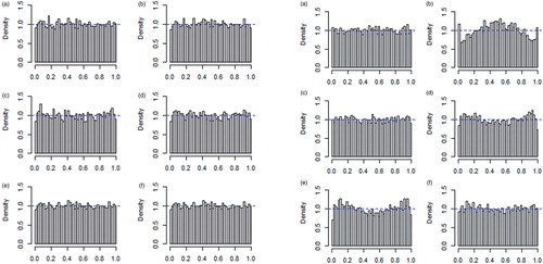
Figure A1: Histograms of the probability integral transform when the true underlying process is white noise (left panel) and ARMA-GARCH (right panel) for; (a) a GARCH-process, (b) white noise process, (c) S&Ö filtered series, (d) HP-filtered series, (e) LLTM filtered series and (f) STM filtered series.

Appendix B. List of tables

Table B1. P-values of diagnostics tests.

Model/Horizon	Unfiltered	LLTM	STM	GARCH(1,1)
LB (1 lag)	0.564	0.961	0.978	0.542
LB (2 lag)	0.133	0.998	0.999	0.421
LB (4 lag)	0.321	0.990	0.994	0.656
LB (6 lag)	0.221	0.931	0.888	0.531
LB (8 lag)	0.364	0.959	0.922	0.698
LB (12 lag)	0.192	0.569	0.504	0.385
LB (24 lag)	0.181	0.480	0.615	0.256
ARCH-LM (1 lag)	0.030	0.210	0.050	0.778
ARCH-LM (2 lag)	0.005	0.448	0.104	0.949
ARCH-LM (4 lag)	0.005	0.770	0.228	0.733
ARCH-LM (6 lag)	0.022	0.633	0.351	0.556
ARCH-LM (8 lag)	0.033	0.760	0.426	0.501
ARCH-LM (12 lag)	0.002	0.931	0.500	0.789
ARCH-LM (24 lag)	0.023	0.407	0.287	0.772
LB-squared (1 lag)	0.030	0.208	0.048	0.778
LB-squared (2 lag)	0.003	0.423	0.081	0.949
LB-squared (4 lag)	0.001	0.750	0.136	0.731
LB-squared (6 lag)	0.004	0.576	0.255	0.539
LB-squared (8 lag)	0.005	0.680	0.356	0.493
LB-squared (12 lag)	0.001	0.835	0.388	0.578
LB-squared (24 lag)	0.007	0.577	0.518	0.770
F-test	0.000	0.999	0.479	0.000
Jarque-Bera	0.000	0.005	0.000	0.000
Shapiro-Wilks	0.000	0.117	0.000	0.005
Kolmogorov-Smirnov	0.006	0.176	0.050	0.810

Note: Numbers are p-values according to respective test in the real data study. The top part of the table shows Ljung-Box tests for whiteness of the residuals, the middle parts shows ARCH-LM and Ljung-Box tests on the squared residuals together with an F-test for equal variances. The bottom part contains tests for normality. Bold fonts indicate statistical significance on the 5% level.

References

- Bollerslev, T. (1986). generalized autoregressive conditional heteroskedasticity. Journal of econometrics, 31(3): 307–327.
- Box, G., and D. Cox. 1964. An analysis of transformations. Journal of the Royal Statistical Society. Series B (Methodological) 26(2):211–52.
- Box, G., and G. Jenkins. 1976. Time series analysis: Forecasting and control, revised ed. Holden-Day.
- Diebold, F., and R. Mariano. 1995. Comparing predictive accuracy. Journal of Business & Economic Statistics 13(3):253–63.
- Diebold, F., T. Gunther, and A. Tay. 1998. Evaluating density forecasts with applications to financial risk management. International Economic Review 39(4):863–83.
- Durbin, J., and S. Koopman. 2012. Time series analysis by state space methods. 2nd ed. Oxford: Oxford University press..
- Engle, R. 1982. Autoregressive conditional heteroscedasticity with estimates of the variance of United Kingdom inflation. Econometrica: Journal of the Econometric Society 50(4):987–1007.
- Granger, C. 1966. The typical spectral shape of an economic variable. Econometrica: Journal of the Econometric Society 34(1):150–61.
- Hamilton, J. 1994. Time series analysis. (Vol. 2). Princeton: Princeton university press.
- Hamilton, J. 2017. Why you should never use the Hodrick-Prescott filter. Review of Economics and Statistics.
- Hodrick, R., and E. Prescott. 1997. Postwar US business cycles: an empirical investigation. Journal of Money, Credit, and Banking 29(1):1–16.
- Jarque, C., and A. Bera. 1980. Efficient tests for normality, homoscedasticity and serial independence of regression residuals. Economics Letters 6(3):255–9.
- Ledolter, J. 2008. Smoothing time series with local polynomial regression on time. Communications in Statistics—Theory and Methods 37(6):959–71.
- Ljung, G., and G. Box. 1978. On a measure of lack of fit in time series models. Biometrika 65(2):297–303.
- Rai, S., B. Abraham, and S. Peiris. 1995. Analysis of short time series with an Ovesr-Dispersion Model. Communications in Statistics – Theory and Methods 24(2):335–48.
- Royston, J. 1982. An extension of Shapiro and Wilk's W test for normality to large samples. Applied Statistics 31(2):115–24.
- Shapiro, S., and M. Wilk. 1965. An analysis of variance test for normality (Complete samples). Biometrika 52(3/4):591–611.
- Smirnov, N. 1948. Table for estimating the goodness of fit of empirical distributions. The Annals of Mathematical Statistics 19(2):279–81.
- Stockhammar, P., and L.-E. Öller. 2012. A simple heteroscedasticity removing filter. Communications in Statistics-Theory and Methods 41(2):281–99.
- Tsay, R. 2010. Analysis of financial time series. New York: Wiley.
- Young, P., C. Ng, K. Lane, and D. Parker. 1991. Recursive forecasting, smoothing and seasonal adjustment of Non-Stationary environmental data. Journal of Forecasting 10(1-2):57–89