On the distribution of Gini’s rank association index

Abstract

Gini’s rank association index is a non parametric measure of association, and is fully described by Genest, Nešlehová and Ben Ghorbal (2010). In this article, we compute the null distribution of this index up to n = 28 where n is the sample size. Our methods are based on permanents and extend the results of Betro (1993). We also discuss approximations to the null distribution for large n. We believe that Gini’s rank association index should be more widely used; in particular, it may be preferable to Spearman’s rank correlation coefficient if the bivariate distribution is such that outliers are quite likely to occur.

Keywords:

• Gini’s gamma
• rank correlation
• hypothesis testing
• exact and approximate distribution
• permanent

1. Introduction

Gini’s rank association index, also known as Gini’s gamma, is a rank correlation coefficient introduced by the Italian statistician, demographer and sociologist Corrado Gini (1914). Let (X₁, Y₁), …, (X_n, Y_n) be a random sample from some continuous bivariate variable (X, Y), with ranks (R₁, S₁), …, (R_n, S_n), respectively. Gini’s gamma is defined to be: (1.1) $${\gamma }_n=\frac{1}{D}\sum _{i=1}^n\left\{\right|(n+1-R_i)-S_i|-|R_i-S_i|\},$$(1.1) $$\mathrm{ }\text{where}\mathrm{ }D=\lfloor n^2/2\rfloor =\{\begin{array}{cc}\frac{n^2}{2},\hfill & \mathrm{ }\text{if}\mathrm{ }n\mathrm{ }\text{is}\mathrm{ }\text{even}\mathrm{ }\hfill \\ \hfill & \hfill \\ \frac{n^2-1}{2},\hfill & \mathrm{ }\text{if}\mathrm{ }n\mathrm{ }\text{is}\mathrm{ }\text{odd}\mathrm{ }\hfill \end{array}.$$

The sum in formula (1.1)(1.1) $${\gamma }_n=\frac{1}{D}\sum _{i=1}^n\left\{\right|(n+1-R_i)-S_i|-|R_i-S_i|\},$$(1.1) may take any value from – D to D, hence γ_n is discretely distributed on the interval $[-1,1].$ In particular, a value of γ_n greater than zero indicates a positive monotonic relationship between X and Y, while a value less than zero indicates a negative relationship. The strength of the relationship depends on how close Gini’s gamma lies to + 1 and −1, respectively, and a value near zero indicates an absence of correlation.

Under the assumption of the independence of X and Y, we have (1.2) $$\mathbb{E}\left({\gamma }_n\right)=0,$$(1.2) (1.3) $$\text{var}\left({\gamma }_n\right)=\{\begin{array}{cc}\frac{2\left(n^2+2\right)}{3(n-1)n^2},\hfill & \mathrm{ }\text{if}\mathrm{ }n\mathrm{ }\text{is}\mathrm{ }\text{even}\mathrm{ }\hfill \\ \hfill & \hfill \\ \frac{2\left(n^2+3\right)}{3(n-1)\left(n^2-1\right)},\hfill & \mathrm{ }\text{if}\mathrm{ }n\mathrm{ }\text{is}\mathrm{ }\text{odd}\mathrm{ }\hfill \end{array},$$(1.3) and that the limiting distribution of $\sqrt{n}{\gamma }_n$ is normal with mean 0 and variance 2/3, as shown by Cifarelli and Regazzini (1977).

As emphasized by Genest, Nešlehová and Ben Ghorbal (2010), Gini’s gamma belongs to the same family of correlation coefficients as the better-known statistics Kendall’s tau and Spearman’s rho. Also included in this family is Spearman’s footrule, a coefficient that is closely related to Gini’s gamma and defined as formula (1.4)(1.4) $${\varphi }_n=1-\frac{3}{n^2-1}\sum _{i=1}^n\left|R_i-S_i\right|.$$(1.4) , (1.4) $${\varphi }_n=1-\frac{3}{n^2-1}\sum _{i=1}^n\left|R_i-S_i\right|.$$(1.4)

The Manhattan (or city block) distance used in Spearman’s footrule and Gini’s gamma is less variable than the Euclidean metric used in Spearman’s rho, as stated by Diaconis and Graham (1977). However, unlike Gini’s gamma, Spearman’s footrule does not behave symmetrically for inverse rankings.

The distribution of γ_n under the assumption of the independence of X and Y has been studied by a number of authors. Savorgnan (1915) tabulated the exact null distribution for $n\le 5,$ Salvemini (1951) extended these results to n = 6 and 7, and Betro (1993) tabulated the null distribution for $n\in \{8,\dots ,15\}.$

In Section 2, we outline the main methods previously used for computing the distribution of Gini’s gamma. In Section 3 we compute the exact distribution of Gini’s rank association index up to n = 28 by the Permanent and BBFG Method. In Section 4 we discuss some approximations to the distribution of Gini’s gamma for large n.

At this point, we mention that Pearson’s correlation coefficient may of course be used to test for independence if (X, Y) follows a bivariate normal distribution (at least approximately). The asymptotic relative efficiencies under bivariate normality of various rank statistics are shown in Table 1 (Genest, Nešlehová and Ben Ghorbal 2010).

Table 1. Asymptotic relative efficiency in the bivariate normal case.

Correlation coefficient	Asymptotic relative efficiency
Spearman’s rank correlation coefficient	${(\frac{3}{\pi })}^2$
Kendall’s rank correlation coefficient	${(\frac{3}{\pi })}^2$
Spearman’s footrule	$\frac{5}{6}{(\frac{3}{\pi })}^2$
Gini’s rank association index	$\frac{8}{9}{(\frac{3}{\pi })}^2$

These rank correlation coefficients are suitable if there may be a monotonic relationship between X and Y. If the possible relationship may be the non monotonic, one may use Hoeffding’s D-test or other tests of a similar form, as described by Hoeffding (1948), Blum, Kiefer, and Rosenblatt (1961), Even-Zohar (2020) and Genest and Rémillard (2004). It should be mentioned that these test statistics do not, of course, give an indication of the direction of any relationship between X and Y (if a monotonic relationship exists).

2. Previous results

To calculate the exact distribution of Gini’s rank association index under the assumption of independence, the simplest algorithm is to enumerate all $n!$ permutations; this will be referred to as the Basic Permutation Method. In this algorithm, the calculation and storage of permutations occupy a lot of time and computer memory. Otten (1973) improved the Basic Permutation Method by splitting the permutations into two sub-permutations, in sets $\{1,\dots ,k\}$ and $\{k+1,\dots ,n\}$ for some integer k between 1 and n. These sub-permutations are processed separately and are followed by addition. Using this algorithm, Otten (1973) extended the exact null distribution of Spearman’s rho to n = 13. The exact distribution of Spearman’s rho was later computed up to n = 26 by Gustafson (2009) using a method based on permanents.

Betro (1993) determined the probability generating function of the Gini’s gamma through a procedure similar to Kendall’s (1962) calculation of Spearman’s probability generating function. The probability generating function was then transformed into an expression related to a permanent. Thus, the calculation of the probability generating function was reduced to calculating the permanent of a matrix A, and the exact distribution of Gini’s gamma was computed by Betro for up to n = 15. It had previously been calculated for smaller n by Savorgnan (1915), Salvemini (1951), and Cifarelli and Regazzini (1977).

3. Computing the distribution of Gini’s gamma up to n = 28

To further extend the exact distribution of Gini’s gamma, we employed Betro’s method (Betro 1993) to construct a modified probability generating function (PGF), and further optimized the computational efficiency to $O(2^{n}n)$ by using the Balasubramanian-Bax-Franklin-Glynn formula rather than Ryser’s formula.

Balasubramanian (1980), Bax (1998), Bax and Franklin (1996), and Glynn (2010) found a formula for calculating permanents: the Balasubramanian-Bax-Franklin-Glynn (BBFG) formula: $$\text{perm}(A)=\frac{1}{2^{n-1}}\left[\sum _{\delta }\left(\prod _{k=1}^n{\delta }_k\right)\prod _{j=1}^n\sum _{i=1}^n{\delta }_i{a}_{ij}\right],$$ where $\delta =({\delta }_1=1,{\delta }_2,\dots ,{\delta }_n)\in {\{\pm 1\}}^n.$

We define the modified PGF for a variable ξ which may take a finite number of integer values (positive, negative, and zero), as: $$F_{\xi }^{*}(z)=\sum _{k=m_1}^{k=m_2}\left[P_{\xi }(k)z^k\right],$$ where $m_1\in \mathbb{Z},m_2\in \mathbb{Z},m_1<m_2,$ and $P_{\xi }(k)$ is the probability that $\xi =k.$

Now we define $M=D\times {\gamma }_n,$ which takes even integer values from –D to D. By methods similar to those used by Cifarelli and Regazzini (1977) to find the PGF of M + D, we find that the modified PGF of M is: $$F_{\xi }^{*}(z)=\frac{1}{n!}\mathrm{ }\text{perm}(A),$$ where A is the n × n matrix with entries $z^{q_{i,j}}$ where $q_{i,j}=(|(n+1-i)-j|-|i-j|)$ for $i,j\in \{1,\dots ,n\}.$

Using the above PGF we implemented the BBFG formula and calculated the distribution of γ_n up to n = 28, using the C++ programming language. We shall call this method for computing the distribution of Gini’s rank association coefficient the Permanent and BBFG Method.

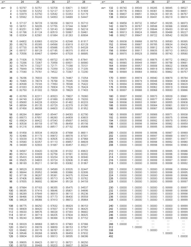
Tables A1–A3 list the cumulative distribution function (CDF) of M for n from 5 to 28, rounded to five decimal places. The values for integer $n\in \{8,\dots ,15\}$ in Table A1 are consistent with those of Betro (1993).

4. Approximations to Gini’s gamma for large n

This section considers two possible approximations for the null distribution of Gini’s gamma: the normal approximation and the Edgeworth approximation.

The mean of γ_n and the variance of γ_n are given by formulae (1.2)(1.2) $$\mathbb{E}\left({\gamma }_n\right)=0,$$(1.2) and (1.3)(1.3) $$\text{var}\left({\gamma }_n\right)=\{\begin{array}{cc}\frac{2\left(n^2+2\right)}{3(n-1)n^2},\hfill & \mathrm{ }\text{if}\mathrm{ }n\mathrm{ }\text{is}\mathrm{ }\text{even}\mathrm{ }\hfill \\ \hfill & \hfill \\ \frac{2\left(n^2+3\right)}{3(n-1)\left(n^2-1\right)},\hfill & \mathrm{ }\text{if}\mathrm{ }n\mathrm{ }\text{is}\mathrm{ }\text{odd}\mathrm{ }\hfill \end{array},$$(1.3) respectively. It follows that the mean of M is 0 and the variance of M is $${\sigma }_M^2=\{\begin{array}{cc}\frac{n^2(n^2+2)}{6(n-1)},\hfill & \mathrm{ }\text{if}\mathrm{ }n\mathrm{ }\text{is}\mathrm{ }\text{even}\hfill \\ \hfill & \hfill \\ \frac{(n^2+3)(n^2-1)}{6(n-1)},\hfill & \mathrm{ }\text{if}\mathrm{ }n\mathrm{ }\text{is}\mathrm{ }\text{odd}\hfill \end{array}.$$

Allowing for a continuity correction of 1, since the values (m) attainable by M are even integers, we may approximate the CDF of the variable M by $\Phi (x),$ where $x=(m+1)/{\sigma }_M,$ and $\Phi$ is the cumulative distribution function of a standard normal random variable. This is the normal approximation.

Allowing for the same continuity correction, the Edgeworth approximation of the variable M is given by $$\Phi (x)-\frac{\beta }{24\sqrt{2\pi }}{e}^{-\frac{1}{2}{x}^2}(x^3-3x),$$ where $\beta =\mathrm{E}({\gamma }_n^4)/{\left[\text{var}({\gamma }_n)\right]}^2-3$ is the kurtosis of γ_n.

Formulae for the fourth moment are given by Landenna, Scagni and Boldrini (1989). We have corrected a suspected typographical error (by changing 107 to 105).

Table 2 compares the normal and Edgeworth approximations to the calculated CDF of M for certain values of m when n = 28. From this, it can be seen that the normal distribution gives a good approximation to Gini’s gamma for n = 28, and therefore it is likely that it would provide a good approximation for n > 28. We can also see that the Edgeworth approximation is extremely accurate, more so than the normal, although the CDF may slightly exceed 1 in certain cases.

Table 2. The calculated CDF of Gini’s gamma for n = 28 with the normal and Edgeworth approximations.

m	Calculated CDF	Normal approximation	Edgeworth approximation	m	Calculated CDF	Normal approximation	Edgeworth approximation
0	0.50637	0.50647	0.50637	160	0.99622	0.99548	0.99616
10	0.56967	0.57078	0.56969	170	0.99784	0.99722	0.99780
20	0.63129	0.63326	0.63133	180	0.99881	0.99833	0.99879
30	0.68980	0.69239	0.68986	190	0.99938	0.99902	0.99937
40	0.74399	0.74690	0.74407	200	0.99969	0.99944	0.99970
50	0.79293	0.79586	0.79303	210	0.99986	0.99969	0.99987
60	0.83603	0.83868	0.83613	220	0.99994	0.99983	0.99995
70	0.87301	0.87517	0.87311	230	0.99997	0.99991	0.99999
80	0.90392	0.90546	0.90399	240	0.99999	0.99995	1.00000
90	0.92906	0.92996	0.92911	250	1.00000	0.99998	1.00001
100	0.94896	0.94925	0.94896	260	1.00000	0.99999	1.00001
110	0.96425	0.96405	0.96423	270	1.00000	0.99999	1.00000
120	0.97567	0.97511	0.97562	280	1.00000	1.00000	1.00000
130	0.98394	0.98317	0.98387	…	…	…	…
140	0.98973	0.98888	0.98965	490	1.00000	1.00000	1.00000
150	0.99365	0.99282	0.99358

5. Conclusions

This article reviews the methods for calculating and approximating the null distribution of Gini’s gamma and extends the tabulation to n = 28. One reason for calculating more exact values of the null distribution of Gini’s gamma is to verify that the normal and Edgeworth approximations are generally reliable. Gini’s gamma is symmetric for inverse rankings and its use of the Manhattan distance implies that it is less variable than statistics that use the Euclidean metric. The tables in the Appendix may be used to construct tests for bivariate independence using Gini’s gamma for n up to 28. The approximations described in Section 4 may be used, with relative confidence, to carry out tests of independence for n larger than 28.

Acknowledgments

We thank Dr. Andreas Grothey (University of Edinburgh) for his valuable advice on code optimization and Prof. Christian Genest (McGill University) for explaining some points. We also thank Liam Bryan and Xueying Liu (Indiana University-Purdue University) for their unpublished project report: A Study of Spearman’s Rank Correlation. Finally, we would like to thank the University of Edinburgh and the University of Bath for the use of their high-powered computer facilities.

Additional information

Funding

Yiwei Zong gratefully acknowledges financial support in the form of a vacation grant from the School of Mathematics and College of Science and Engineering at the University of Edinburgh. Ffion Loring gratefully acknowledges financial support in the form of a vacation grant from MAC-MIGS at the Maxwell Institute Graduate School.

Appendix A

Table A1. The CDF of M for $5\le n\le 18.$

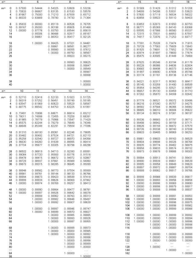
Table A2. The CDF of M for $19\le n\le 23.$

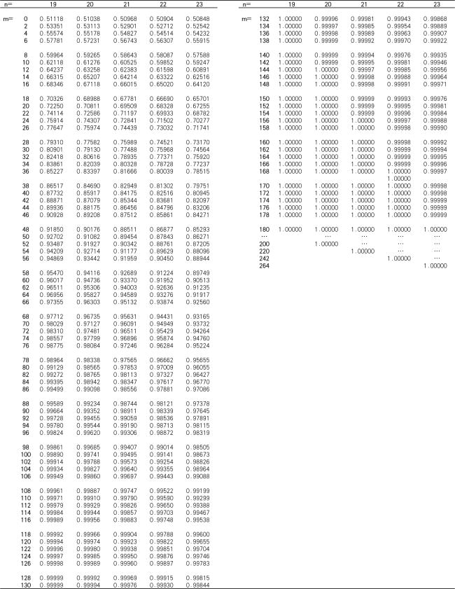
Table A3. The CDF of M for $24\le n\le 28.$

References

- Balasubramanian, K. 1980. Combinatorics and diagonals of matrices. Thesis, Indian Statistical Institute, Calcutta.
- Bax, E. T. 1998. Finite-difference algorithms for counting problems. Thesis. California Institute of Technology, Pasadena, CA.
- Bax, E. T., and J. Franklin. 1996. A finite-difference sieve to count paths and cycles by length. Information Processing Letters 60 (4):171–6. doi:10.1016/S0020-0190(96)00159-7.
- Betro, B. 1993. On the distribution of Gini’s rank association coefficient. Communications in Statistics - Simulation and Computation 22 (2):497–505. doi:10.1080/03610919308813105.
- Blum, J. R., J. Kiefer, and M. Rosenblatt. 1961. Distribution free tests of independence based on the sample distribution function. The Annals of Mathematical Statistics 32 (2):485–98. doi:10.1214/aoms/1177705055.
- Cifarelli, D. M., and E. Regazzini. 1977. On a distribution-free test of independence based on Gini’s rank association coefficient. Recent Developments in Statistics (Proceedings of the European Meeting of Statisticians, Grenoble 1976), Amsterdam, North Holland, 375–85.
- Diaconis, P., and R. L. Graham. 1977. Spearman’s footrule as a measure of disarray. Journal of the Royal Statistical Society: Series B (Methodological) 39 (2):262–8. doi:10.1111/j.2517-6161.1977.tb01624.x.
- Even-Zohar, C. 2020. Independence: fast rank tests. arXiv preprint arXiv: 2010.09712. doi:10.48550/arXiv.2010.09712.
- Genest, C., and B. Rémillard. 2004. Tests of independence and randomness based on the empirical copula process. Test 13 (2):335–69. doi:10.1007/BF02595777.
- Genest, C., J. Nešlehová, and N. Ben Ghorbal. 2010. Spearman’s footrule and Gini’s gamma: A review with complements. Journal of Nonparametric Statistics 22 (8):937–54. doi:10.1080/10485250903499667.
- Gini, C. 1914. L’Ammontare e la Composizione della Ricchezza delle Nazione. Torino: Bocca.
- Glynn, D. G. 2010. The permanent of a square matrix. European Journal of Combinatorics 31 (7):1887–91. doi:10.1016/j.ejc.2010.01.010.
- Gustafson, L. 2009. Spearman’s rho null distribution. Last modified September 6. https://luke-g.com/math/spearman/index.html (accessed August 6, 2021).
- Hoeffding, W. 1948. A non-parametric test of independence. The Annals of Mathematical Statistics 19 (4):546–57. doi:10.1214/aoms/1177730150.
- Kendall, M. G. 1962. Rank correlation methods: 3d Ed. C. Griffin. Statistics 19:546–57.
- Landenna, G., A. Scagni, and M. Boldrini. 1989. An approximated distribution of the Gini’s rank association coefficient. Communications in Statistics - Theory and Methods 18 (6):2017–26. doi:10.1080/03610928908830019.
- Otten, A. 1973. The null distribution of Spearman’s S when n=13(1)16. Statistica Neerlandica 27 (1):19–20.
- Salvemini, T. 1951. Sui vari indici di cograduazione. Statistica 11:133–54.
- Savorgnan, F. 1915. Sulla Formazione dei Valori dell’Indice di Cograduazione. Studi Economico-Giuridici dell’Università di Cagliari.
Appendix A
Table A1. The CDF of M for
Table A2. The CDF of M for
Table A3. The CDF of M for