Supply and demand macro-econometric model of a small economy: evidence from Namibia

ABSTRACT

This study develops a macro-econometric model for the Namibian economy. This macro-econometric model estimates both the demand and supply sides of the Namibian economy. This model incorporates the price sector, in order to serve as a link between the supply and demand sides of the economy. The model consists of behavioural equations, linked by identities and definitions. These behavioural equations were estimated and simulated individually. They were then combined together to form a full macro-econometric model of the Namibian economy. The full macro-econometric model was closed using two models. The first model activates the supply side and marginalises the demand side. The second model is demand side orientated, which activates the demand side and marginalises the supply side. The results indicate that the estimated values closely approximate the actual values. This macro-econometric model can be used to apply policy simulations, in order to determine appropriate economic policies for Namibia.

KEYWORDS:

• Macro-econometric
• supply-side
• demand-side
• cointegration
• stationarity

JEL CLASSIFICATION:

• C51
• C52
• C53
• E00

1. Introduction

Namibia has achieved a moderate growth rate of 4.9% during the period 1990–2012. It has also achieved macroeconomic stability during the same period. However, the average moderate growth rate of 4.9% is below the target of 7% which is required to alleviate poverty and ensure that the country achieves a standard of living comparable to the developed countries by the year 2030. The moderate growth rate and macroeconomic stability were not sufficient to reduce unemployment and further accelerate poverty reduction. Unemployment has been on an increasing trend, especially from the late 1990s to 2011. The real GDP declined in 2009 by 0.7%, while the unemployment rate increased to 36%. The rise in unemployment is attributed to the fact that the growth rate is just moderate and not high enough to generate the much-needed jobs. The country has excess savings over investment. The excess savings have resulted in capital outflows, mainly to South African financial markets. This situation is not typical of a developing country and indicates that Namibia has not been able to convert these excess savings into investment projects that can accelerate economic growth and provide employment to the increasing labour force. This raises an important question on what can be done to accelerate economic growth and reduce the high unemployment rate.

There is a need for an economic framework that captures the underlying characteristics of the Namibian economic environment. This will assist in analysing various policy interventions that will generate high economic growth and reduce unemployment. A macro-econometric model is a useful tool in analysing factors and policies that can generate high economic growth and reduce unemployment. In light of the above, the objective of this study is to develop and estimate a macro-econometric model for the Namibian economy. The model is on both supply and demand sides of the economy. This could assist in providing a long-term solution to accelerate economic growth and reduce the rising unemployment. Specifically, the study focuses on the following:

• Supply side modelling, which represents an economy with structural constraints. GDP is estimated in this model in order to identify constraints that impede economic growth and development. If there is a limited capacity to absorb labour in the economy, it results in higher unemployment.

• Demand side modelling, where the economy has limited or no supply constraints. GDP in this model is estimated following the Keynesian identity. According to this Keynesian identity, intervention in the economy through fiscal and monetary policies could be effective in accelerating capital investment and absorbing labour.

• The study, therefore, tests if there are structural supply and demand constraints which discourage growth and development of the country.

• Comparing the demand and supply models will help in identifying factors that impede the development of the economy.

• Policy simulations, in order to test the responsiveness of endogenous variables to shocks on selected exogenous variables.

This paper will rely on policy implications to be done through shocks or impulse response analysis. The study will showcase the dynamics of the Namibian macro-economy. That is an economic environment that has structural supply side constraints compared to demand side constraints. To my best knowledge, this will be the first study in this area on the Namibian economy. This study, therefore, serves as a baseline for a series of papers that rely heavily on the policy implications of various shocks on the Namibian economy. The rest of the study is organised as follows: Section 2 provides a brief overview of the Namibian economy. Section 3 discusses the theoretical framework (theoretical models to be estimated). Section 4 explains the empirical framework and outlines the econometric methodology, as well as data to be used for estimation of the model. The empirical results are presented in Section 5, while Section 6 concludes.

2. Brief overview of the Namibian economy

2.1. Growth trends and GDP by sector

Since Namibia gained independence in 1990, the government has placed great emphasis on boosting economic growth. The two most important parts of the government strategy to create employment opportunities and address the socio-economic imbalances inherited from the colonial times are diversification of the economy and development of the agricultural and manufacturing sectors. Real GDP growth for the period 1990–2012 is plotted in Figure 1, which shows that Namibia recorded moderate growth rates during the period 1990–2012. A negative real GDP growth rate of −0.7 was recorded in 2009 and this is attributed to the global economic crisis of 2008–2009. The average real GDP growth rate for the period 1990–2011 was 4.9%. This average real GDP growth rate is below the 7% growth target under Vision 2030. According to the National Planning Commission (2004), Vision 2030 is a vision that will guide Namibia to make deliberate efforts to improve the quality-of-life of its people to the level of their counterparts in the developed world by the year 2030. The 7% real GDP growth rate per year is required in order to achieve the target of Vision 2030. The real GDP per capita growth tracked that of real GDP during the same period. It has always been below that of real GDP. However, it was slightly higher than that of real GDP. This may suggest that there was a decline in population growth, but data from the National Planning Commission indicates that the population grew by 2%.

Figure 1. Real GDP and real GDP per capita growth rates.

Source: Data obtained from the Bank of Namibia.

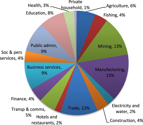
The composition of Namibia’s GDP shows that the economy is dominated by tertiary industries (such as wholesale and retail trade, hotels and restaurants, transport and communications, financial and business services, education, health and government), which accounted for an average of 57% during 1990–2009. Trade, government and business services accounted for the largest shares of the tertiary (services) sector. The secondary sector comprises manufacturing, electricity & water and construction, and accounted for an average of 16% of the GDP during 1990–2009. Although the contribution of manufacturing to GDP increased from 10% in 1990 to 14% in 2012, Namibia still has a small manufacturing base. The manufacturing sub-sector is dominated by meat processing, fish processing and beverages.

The primary sector, which consists of agriculture, forestry, fishing and mining, accounted for an average of 20% of GDP during the period 1990–2012. The main contribution in this sector came from mining and quarrying. Although the Namibian economy is more diversified than many others in sub-Saharan Africa, further diversification remains a main component of government policy. More efforts are still needed to diversify the economy from the traditional sectors and develop other industries such as manufacturing. Diversification of the economy has the potential to contribute to economic growth and generate the much-needed employment as well as poverty alleviation (Figure 2).

Figure 2. Sectoral contribution to GDP (average, 2005–2012).

Source: Data for the figure are obtained from the Bank of Namibia.

2.2. Savings and investment trends

2.2.1. Aggregate saving and investment to GDP

Gross domestic savings is defined as the difference between gross national disposable income and final consumption expenditure; i.e. income that is not consumed is saved. If a country spends its national income on consumption, there will be fewer resources available for savings and for investment. However, while domestic savings are the main source of finance for investment, domestic savings and investment may not be equal. The difference between savings and investment reflects the foreign savings position of the country. If there is excess savings over investment, it will result in foreign lending and this will be reflected in an outflow of capital. However, if national savings are deficient (less than investment) it will lead to import of capital through foreign borrowing.

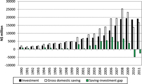
The trends in savings and investment are plotted in Figure 3. Namibia experienced excess savings over investment for the period 1990–2009, reflected in surpluses on the current account of the balance of payments. The gap between savings and investment reached its highest level of N$7.5 billion in 2006. The global economic crisis caused excess savings to fall to a relatively low level of N$3.8 billion in 2009, as overall savings declined.

Figure 3. Saving, investment and saving–investment gap (Namibia dollar N$ million).

Source: Computed using data from the Bank of Namibia.

Savings, investment and saving-investment gap as ratios of GDP are plotted in Figure 4. The excess of saving over investment is a particular characteristic of the Namibian economy, and shows that Namibia has not been able to use its entire savings for investment. The excess saving led to capital outflows or lending to other countries, especially to the South African financial markets. The highest ratio of saving to GDP was recorded in 2006 and 2008. It increased from 30% in 2005 to 35% in 2006, before declining slightly to 34% in 2008. According to the Bank of Namibia (2009), the increase in saving is attributed better fiscal management and strong growth in tax revenue, which led to an increase in general government gross saving during that period. The average ratio of saving to GDP during 1990–2009 was 27%. However, a negative saving investment gap emerged during the last 3 years (2010–2013). The savings investment gap became negative for that period. This means that Namibia is starting to convert all the savings into investment.

Figure 4. Domestic savings, investment and the saving–investment gap (percentage of GDP).

Source: Data obtained from the Bank of Namibia.

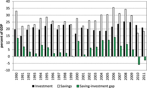
Although Namibia has not been able to turn its abundance of savings into investment (except for the period 2010–2013), the average investment to GDP ratio was 20% during the same period (see Figure 4). The average excess saving over investment or saving-investment gap was 6.6 of GDP during 1990–2009. The Bank of Namibia (2009) states this ratio is expected to increase over the next few years as the economy recovers from the global economic crisis. The continued excess of savings over investment suggests that measures aimed at curbing capital outflows have not been particularly successful at boosting investment in the local economy.

2.3. Unemployment rate

Unemployment rate is plotted in Figure 5. This figure shows that unemployment has been on an increasing trend between 1971 and 1985. It decreased and stabilised between 1987 and 1999. It increased sharply between 2000 and 2009. Unemployment increased to 36% in 2009. Although Namibia achieved moderate growth during the period 1990–2012, it was not sufficient to generate much-needed jobs and unemployment rate continued to increase.

Figure 5. Unemployment rate. Data for the figure sourced from Hartmann (1988) and the Ministry of Labour and Social Welfare (1997, 2000, 2002, 2004, 2008).

3. Theoretical framework

The focus of this macro-econometric model is to test the hypothesis that there exist supply constraints vs the demand constraints and these impact negatively on economic growth and development. It also investigates simulations of different policies, in order to recommend appropriate policies for the country.

If an economy is characterised by capacity constraints, the domestic production will not be sufficient to satisfy domestic demand. In such an economy, an increase in domestic expenditure (instead of an increase in domestic production) will fuel GDP and the economy will not be able to generate the much-needed jobs and alleviate poverty (Akanbi & Du Toit, 2011). An economy with structural capacity constraints will not be able to absorb more labour and this results in rising unemployment. Such an economy requires policies that are aimed at eliminating structural capacity constraints.

On the other hand, if an economy does not have structural capacity constraints, monetary and fiscal policies can be used to increase employment. Fiscal and monetary policies would be effective in raising GDP and increase labour employment in this case. Expansionary monetary and fiscal policies will result in higher GDP and appropriate distribution of income among the owners of factors of production (Akanbi & Du Toit, 2011).

Following Akanbi and Du Toit (2011), Akanbi (2013), Musila (2002) and Musila & Rao (2002), this study proceeds as follows:

• Estimate the supply side model, which marginalises the demand side. This model assumes that the economy has structural capacity constraints. The supply side model estimates GDP in order to investigate the constraints to growth and development of the country. As previously explained, an economy with structural capacity constraints has limited capacity to generate jobs and absorb labour into the economic system. This results in high unemployment and poverty.

• Develop a demand side, which marginalises the supply side. This model assumes that the economy does not have structural capacity constraints. Fiscal and monetary policies in this economy will be effective in accelerating economic growth and job creation. This helps in attracting investment and to absorb labour into the economy. This model estimates GDP using the Keynesian definition (identity).

• Policy simulations through a few shocks or impulse response analysis on the macro-economic variables of the Namibian economy. It would have been appropriate for this study to rely heavily on the policy implications of various shocks to the Namibian economy. However, this study develops baseline models for further research papers on the policy implications of various shocks to the Namibian economy. A detailed policy implication of the various shocks on the Namibian economy is not included. If a detailed policy analysis were to be included, the page or word limitation of the journal would be exceeded. It is also important to indicate that a detailed policy analysis of the shocks falls outside the scope of this paper.

The macroeconometric model developed in this study consists of real, external, monetary and price sectors. It has behavioural equations, identities and definitions. It captures the long-run and short-run features of the economy. The equations from the four sectors of the economy are specified as follows.

3.1. Real sector

The components of the real sector are aggregate supply, aggregate demand and prices. By estimating the production function, investment, labour and wages, aggregate supply determines the real output of the economy. The price sector determines the consumer prices, while consumption expenditure in the economy is determined by aggregate demand.

3.1.1. Production function

This is a neoclassical theoretical framework and the study adopts the Cobb-Douglas production (Cobb & Douglass, 1928). It is based on the assumption of constant returns to scale for labour and capital inputs. Constant returns to scale suggests that, if the amount of inputs is doubled, output will also double. Despite criticism in the theoretical literature (such as Barro, 1990, 1991), neoclassical models are still used extensively to estimate macro-econometric models of both developed and developing countries. The formulation of aggregate supply function relates output to the inputs of capital and labour, as well as technological progress. Total output is modelled using the Cobb-Douglas production function with constant returns to scale. It is specified as follows:(1) where Y, K, A and L are output, capital, technological progress and labour, respectively. Equation (1) is estimated in log-linearised form. Capital and labour are expected to have a positive impact on the level of output. However (as pointed out by Damoense-Azevedo, 2013 and Musila, 2002), they exhibit diminishing returns, and this suggests that technological progress is required to accelerate economic growth.

3.1.2. Demand for labour

The demand for labour equation is specified as:(2) where L, Y, W and PROD are labour or employed people, real output (real GDP), wages and labour productivity, respectively. Labour productivity is computed as output divided by labour. An increase in real output is expected to increase the demand for labour. A rise in wages and labour productivity can cause the demand for labour to decrease. The coefficients of real output are expected to be positive, while those of wages and labour are expected to be negative. However, it is also possible for the coefficient of productivity to be negative because, if existing workers are more productive, there will be less need to hire more labour.

3.1.3. Wages

Wages are determined by labour productivity and the price level, and the equation is estimated as:(3) where PROD is computed as:

Consumer prices and a rise in labour productivity have a positive impact on wages.

3.1.4. Investment

Investment is estimated according to the neoclassical model of domestic investment. This is based on Jorgenson (1963). The investment function is determined by the user cost of capital, savings, real output and the level of financial development. The equation is specified as follows:(4) Where UCC, S and Y are user cost of capital, savings and real output, respectively. The user cost of capital is computed following Eita and Du Toit (2009). The user cost of capital impacts negatively on investment. An increase in user cost of capital is expected to increase the cost of financing investment (Akanbi & Du Toit, 2011; Eita & Du Toit, 2011). A rise in savings and real GDP are expected to impact positively on investment.

3.1.4.1. Capital stock

Capital stock is computed as:(5) where K and dep are capital stock and rate of depreciation, respectively. INV is as defined before.

3.1.5. Consumption

Consumption (CONS) is a function of disposable income (YD), wealth (W) and real interest rate (RI). The consumption function is, therefore, specified as:(6) Disposable income and wealth are expected to positively impact on consumption. However, consumption is expected to respond negatively to interest rates.

3.2. Prices

The price levels (consumer prices) are determined by wages, exchange rate, nominal user cost of capital, excess demand and import prices. The price equation is specified as:(7) where P, EXCH, EXD and SAPPI are consumer prices, exchange rate, excess demand and import prices proxied by the South African Producer Price Index. UCC and W are as previously defined. Increases in these variables are expected to drive up consumer prices.

3.3. External sector

3.3.1. Export of goods and services

Exports of goods and services is determined by foreign income (Y*), exchange rate (EXCH) and relative prices (P/P*). Export of goods and services are specified as:(8) where X, Y^w, EXCH and P/P* are export, foreign (world) income, exchange rate and domestic prices relative to foreign prices, respectively. A rise in foreign income and depreciation of the exchange rate are expected to promote export. An increase in domestic relative to foreign prices is expected to cause a reduction in exports.

3.3.2. Import of goods and services

Imports of goods and services in the economy is determined by domestic income (Y), relative prices (P/P*) and exchange rate (EXCH). It is specified as follows:(9) A rise in domestic income is expected to cause an increase in imports. An increase in domestic prices relative to foreign prices and depreciation of the exchange rate are expected to cause a reduction in imports.

3.4. The monetary sector

The kernel of monetary sector modelling is to obtain information on the extent to which monetary variables play a role in the rest of the economy (see Akanbi & Du Toit, 2011). Determination of the interest rate is done by invoking the assumption that financial markets clear immediately. If that is the case, money demand and money supply will be equal, because the interest rate adjusts in order to bring equilibrium to the market. The interest rate is, therefore, determined by inverting the standard money demand equation. The interest rate equation is determined as:(10) where IR, MD and P are interest rate, monetary aggregate and inflation rate, respectively. Money demand is a positive function of income and negatively related to the interest rate. The interest rate is positively related to income and prices, but negatively related to money demand.

4. Empirical framework

4.1. Econometric methodology

The availability of data determines the appropriate econometric methodology to be employed. This study uses a dataset that has few observations, and this means that a number of feasible econometric methods are limited. This is a time-series econometric study. The study adopts the Engle-Granger two steps econometric methodology. This econometric methodology is widely used in the literature of macro-econometric modelling. It is useful in the sense that it avoids the problem of spurious regression. Spurious regression gives an impression of good econometric results, even though there is no meaningful relationship between variables.

Despite its potential defects, the Engle and Granger (1987) two steps method was chosen to estimate the supply side macro-econometric model of the Namibian Economy. This technique involves estimation of the long-run cointegrating or economic equilibrium relationship between variables by means of testing stationarity of the residuals. The Augmented Dickey Fuller (ADF) test statistic is employed to test if the residuals from the long-run equation are stationary. The null hypothesis of no cointegration is tested by comparing the ADF statistic with MacKinnon critical values. If the null hypothesis of no cointegration is rejected, then there is cointegration. An error correction model (ECM) consisting of stationary residuals from the long-run cointegration equation can be estimated. The stationary residuals must be lagged by one period and is expected to have a negative sign. This allows for the system to adjust towards long-run equilibrium. The coefficient of the ECM represents the speed of adjustment of the system to equilibrium. It indicates the number of times required for the system to return to equilibrium. Policy implications of the various shocks to the Namibian economy will be simulated.

4.2. Data

This is a time series data analysis study. It uses annual data for the period 1980–2012. The description and sources of data used in the study are presented in Table 1.

Table 1. Data sources and description.

Variable	Variable description	Source
lnCONS	Final consumption expenditure	Central Bureau of Statistics; Bank of Namibia
lnP	Consumer price index	Bank of Namibia, Hartmann (1988); Central Bureau of Statistics
dep	Rate of depreciation	Bank of Namibia; Hartmann (1988); Cornwell et al. (1991)
lnEXCH	Nominal exchange rate (N$/USA$)	Central Bureau of Statistics and Bank of Namibia
DUM88	Dummy variable for political and economic uncertainty in 1987–89 (value of 1 in 1987–89 and 0 elsewhere)	Computed
DUMIND	Dummy for Namibia’s independence in 1990 (it takes value of 0 before 1990 and 1 after 1990)	Computed
DUMMIN	Dummy variables for the significant investment in the mining sector for the period 2001–03	Computed
lnEXCH	Exchange rate of the Namibia dollar (N$) to the USA dollar	Bank of Namibia; IMF’s International Financial Statistics
lnEXD	Excess demand computed as	Computed from data obtained from Bank of Namibia; Hartmann (1988)
lnIMP	Import prices proxied by import price index	Computed using data sourced from Bank of Namibia; Hartmann (1988); Cornwell et al. (1991)
lnINDPRO	Industrial production index in advanced economies as proxy for foreign or world income	OED database; IMF’s International Financial Statistics
lnIR	Interest rate (proxied by lending rate)	Bank of Namibia; IMF’s International Financial Statistics
lnINV	Investment (gross fixed capital formation)	Bank of Namibia; Hartmann (1988); Cornwell et al. (1991)
lnGNDI	Real gross national disposable income	Central Bureau of Statistics
lnK	Fixed capital stock	Bank of Namibia, Hartmann (1988); Cornwell et al. (1991)
lnL	Labour or the number of people employed	Bank of Namibia; Hartmann (1988); Cornwell et al. (1991); Ministry of Labour and Social Welfare (1997, 2000, 2004, 2008); World Bank Development Indicators
lnM	Imports of goods and services	Bank of Namibia; Central Bureau of Statistics
lnWL	Monetary aggregate proxied by M2. It is used as proxy of wealth	Bank of Namibia, IMF’s International Financial Statistics
lnMD	Real monetary aggregates (M2)	Bank of Namibia, IMF’s International Financial Statistics
lnP	Consumer Price Index	Bank of Namibia; Hartmann (1988); Cornwell et al. (1991)
ΔP or inflation rate	Inflation rate	Computed
Pk	Price of capital proxied by investment deflator	Computed using data from Central Bureau of Statistics; Bank of Namibia
(lnRELPRICE)	Relative prices. Namibia’s consumer price index (P) relative to world price index (P*).	Data for Namibia’s consumer price index were sourced from the Central Bureau of Statistics of Namibia. Data for the world price index were obtained from the IMF’s International Financial Statistics
lnPROD	Labour productivity computed as	Computed using data from Bank of Namibia; Hartmann (1988); Cornwell et al. (1991); Ministry of Labour and Social Welfare (1997, 2000, 2004, 2008); World Bank Development Indicators
lnREER	Real exchange rate	Bank of Namibia
lnRW	Real wages (real remuneration of employees in the Namibian economy)	Central Bureau of Statistics; Hartmann (1988); Cornwell et al. (1991)
lnS	Savings (gross domestic savings)	Bank of Namibia; Hartmann (1988); Cornwell et al. (1991)
lnUCC	User cost of capital computed following Eita and Du Toit (2009)	Computed using the data from Bank of Namibia; Hartmann (1988); Cornwell et al. (1991). It is computed as:
lnW	Nominal wages (proxied by remuneration of employees in the Namibian economy)	Bank of Namibia; Hartmann (1988); Cornwell et al. (1991)
lnRW	Real wages	Computed by deflating remuneration of employees
lnSAPPI	South African Producer Price Index	South African Reserve Bank
T	Time trend	Computed
trate	Tax rate (proxied by tax revenue as ratio of nominal GDP)	Computed using data from Central Bureau of Statistics, Bank of Namibia
lnX	Exports of goods and services	Bank of Namibia; Central Bureau of Statistics
lnY	Real GDP	Bank of Namibia; Hartmann (1988); Cornwell et al. (1991)
LnY^W	Foreign income (proxied by industrial production of advanced economies)	Sourced from OECD database. The data base is available on OECD website.

5. Empirical results

5.1. Unit root test results

Univariate characteristics of the data which involves unit root test is the first step before estimation of the equations. This study uses ADF test and Phillips-Perron (PP) test statistics to establish the univariate characteristics of the data. These two test statistics have been criticised that they have low power, in the sense that they sometimes under-reject the null hypothesis of the unit root, even when the variable is stationary. A more powerful test for unit root, Kwiatkowski-Phillips-Schmidt-Shin (KPSS), is also used in this study in order to ensure that the results are robust. The unit root test results are presented in Table 2. The results in Table 2 indicate that, according to ADF and Phillips-Perron (PP) test statistics, variables are non-stationary (contain unit root) in levels, but become stationary on first differences (with the exception of three variables). This means that the null hypothesis of unit root is not rejected for variables in levels. The null hypothesis is rejected for variables for all variables in first differences. The results of KPSS statistic which uses the null hypothesis of stationarity (no unit root) show that the null hypothesis of stationarity is rejected for all variables in levels. This null hypothesis of stationarity is not rejected for variables in first differences. This indicates that, according to KPSS test statistic, variables are non-stationary in levels, but become stationary on first differences. KPSS results are consistent with those of ADF and PP.

Table 2. Unit root test results.

		Levels			First difference
Variable	Model	ADF	PP	KPSS	ADF	PP	KPSS
ln	Constant Constant & trend none	1.53 −1.98 2.97	−0.20 −2.13 3.81	0.73## 0.19##	−7.84*** −8.38*** −0.26	−7.97*** −23.78*** −6.21***	0.15 0.13
ln	Constant Constant & trend none	−0.29 −2.05 1.42	−0.99 −2.03 2.56	0.78### 0.12#	−2.38 −2.32 −1.88*	−2.43 −2.29 −1.84*	0.18 0.18
ln	Constant Constant & trend none	−0.68 −2.23 1.15	−0.66 −2.30 1.09	0.73### 0.09	−5.64*** −5.54*** −4.99***	−5.60*** −5.48*** −4.50***	0.10 0.10
ln	Constant Constant & trend none	−2.64* −2.42 −0.88	−1.93 −1.59 −0.84	0.43# 0.15##	−4.20*** −4.48*** −4.09***	−4.23*** −4.91*** −4.24***	0.16 0.08
ln	Constant Constant & trend none	1.18 −0.47 3.84	1.53 −0.52 3.80	0.76### 0.16##	−4.91*** −5.01*** −3.77***	−4.87*** −4.91*** −3.74***	0.27 0.14
ln	Constant Constant & trend none	−1.88 −2.87 −0.40	−1.57 −2.21 −0.49	0.24 0.15##	−3.15** −3.50* −3.19***	−3.09** −3.47* −3.12***	0.39 0.17
ln	Constant Constant & trend none	−2.32 −1.43 4.67	−2.75* −1.34 3.56	0.76### 0.18##	−5.98*** −7.02*** −1.96**	−6.00*** −7.06*** −3.53***	0.46 0.06
ln	Constant Constant & trend none	−2.09 −1.78 −0.46	−1.90 −1.36 −0.35	0.26 0.21##	−4.96*** −5.43*** −5.04***	−4.84*** −8.55*** −4.95***	0.31 0.34
ln	Constant Constant & trend none	0.02 −0.88 1.55	0.18 0.78 1.66	0.48## 0.17##	−5.45*** −6.78*** −6.22***	−6.45*** −6.79*** −6.21***	0.26 0.10
ln	Constant Constant & trend none	0.53 −0.92 2.41	0.31 −1.24 7.28	0.75### 0.17##	−3.03** −2.87 −1.32	−2.86* −2.68 −1.82*	0.16 0.11
ln	Constant Constant & trend none	1.82 −3.45* 2.68	2.86 −1.64 3.00	0.69## 0.20	−4.29** −5.27*** −3.86***	−4.23*** −7.46*** −3.92***	0.37 0.29###
ln	Constant Constant & trend none	−1.20 −1.17 6.72	−1.26 −1.11 6.31	0.74### 0.15##	−5.79*** −6.11*** −2.54**	−5.79*** −6.09*** −2.39**	0.20 0.08
ln	Constant Constant & trend none	−0.41 −2.39 2.53	−0.32 −2.39 3.04	0.72## 0.08	−6.26*** −6.14*** −5.02***	−6.29*** −6.16*** −5.06***	0.09 0.09
ln	Constant Constant & trend none	−5.86*** 0.05 0.96	−5.63*** 0.21 4.99	0.74### 0.20###	−2.37 −4.31*** −0.11	−2.30 −4.36*** −1.12	0.43 0.20
ln	Constant Constant & trend none	−1.52 −0.29 −1.53	−1.69 −0.48 −1.71	0.28 0.19##	−3.15** −3.93** −3.20***	−3.08*** −3.92** −3.13***	0.453 0.11
ln	Constant Constant & trend none	−1.13 −2.72 1.60	−0.87 −2.69 2.71	0.82### 0.14##	−5.93*** −5.87*** −5.44***	−5.60*** −5.92*** −5.46***	0.16 0.15
ln	Constant Constant & trend none	0.09 −1.65 3.18	0.09 −1.53 3.18	0.71## 0.17##	−6.13*** −6.36*** −4.96***	−6.23*** −6.36*** −5.02***	0.13 0.06
ln	Constant Constant & trend none	−2.18 −2.66 0.11	−2.02 −2.54 0.69	0.36# 0.17##	−8.29*** −8.21*** −8.34***	−9.26*** −10.22*** −9.04***	0.30 0.47##
ln	Constant Constant & trend none	−1.96 −0.44 1.595	−2.19 0.02 1.15	0.71### 0.18###	−5.00*** −5.51*** −4.15***	−5.00*** −5.84*** −4.15***	0.46 0.14
ln	Constant Constant & trend none	1.67 0.74 1.81	0.98 −0.83 2.88	0.77### 0.10	−1.94 −2.06 −1.12	−2.05 −1.84 −0.55	0.24 0.15
ln	Constant Constant & trend none	−0.08 −3.87* 1.65	0.59 −4.10** 2.79	0.714### 0.20##	−5.80*** −5.73*** −5.25***	−9.31*** −11.71*** −5.25***	0.31 0.27
ln	Constant Constant & trend none	2.10 −2.39 6.04	2.53 −3.24* 6.03	0.73## 0.18##	−4.37*** −5.15*** −2.45**	−4.32*** −5.66*** −2.45**	0.55 0.17
ln	Constant Constant & trend none	−0.95 −1.96 2.77	−1.04 −2.13 3.81	0.72## 0.14#	−5.19*** −5.19*** −4.25***	−5.47*** −6.16*** −4.23***	0.19 0.16
lnSAPPI	Constant Constant & trend none	−4.07*** −1.39 1.97	−4.37*** −1.40 4.95	0.74### 0.19##	−3.22** −4.06** −1.40	−3.19** −3.89** −1.22	0.60 0.11

Notes: KPSS uses the null hypothesis of stationary (no unit root), while ADF and PP use the null hypothesis of non-stationary (there is unit root).

#, ## and ### indicate rejection of the null hypothesis of stationary (no unit root) at 1%, 5% and 10% significance levels, respectively.

*, ** and *** indicate rejection of the null hypothesis of non-stationarity (there is unit root) at 1%, 5% and 10% significance level, respectively.

5.2. Estimation results

5.2.1. Production

The results of equation (1), shown in Table 3, indicate that a 1% increase in capital stock causes real GDP to increase by 0.13%. An increase in labour by 1% causes real GDP to increase by 0.87%. These results show that labour is the main contributor to growth in output. These results are consistent with theoretical expectations. The null hypothesis of no cointegration was rejected because the residuals from the long-run equation are stationary. This means that the variables are cointegrated and it is appropriate to proceed to the error correction model or short-run estimation. The short-run results in Table 3 show that the coefficient of the ECM is negative and statistically significant. The ECM coefficient represents the speed of adjustment. It indicates that there is adjustment to equilibrium. It shows that 37% of disequilibrium is corrected every year. The short-run results passed all diagnostic statistics (such as normality, heteroscedasticity, autocorrelation, stability, serial correlation), suggesting that there is no violation of the assumptions of the classical linear regression model. The next step is to simulate the model in equation (1), and the results are presented in Figure 6. Figure 6 shows that the model is a good fitm because the estimated real GDP track the actual GDP.

Figure 6. Actual and estimated real GDP.

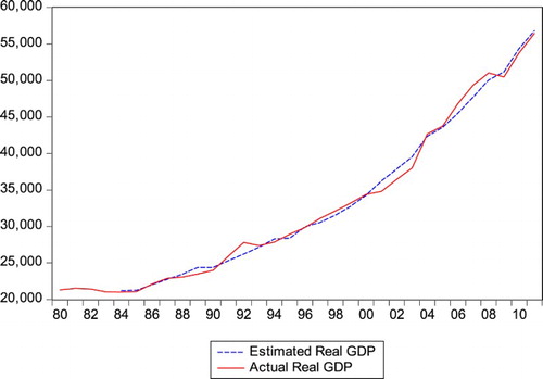
Table 3. Long-run and short run results of the real sector.

Long-run results
Explanatory variables	Dependent variables
Constant	−2.2***		6.65***	−13.7***	3.97***
	0.13**
	0.87***
		−0.71***
		1.91***		1.89***
					0.57***
			0.20***
			0.25
				0.03
				0.71
					−0.02***
					0.06
				−0.45***
		−0.02
		−0.26***		0.43**
			0.16***
			0.11***
R-squared	0.98	0.83	0.98	0.92	0.89
Adjusted R-squared	0.98	0.81	0.98	0.90	0.88
Short-run results
Explanatory variables	Dependent variables
	0.01	0.02**	0.08**	−0.09***	0.06**
	−0.37***	−0.12**	−0.92***	−0.58***	−0.45***
	−0.29*	−0.38**
	−1.40***
				−0.08***
		0.51***		1.11*
			−0.30*
			0.85**
					0.23
					−0.01*
					−0.25*
			0.07**
				0.13***
	0.003***
R-squared	0.44	0.39	0.44	0.73	0.41
Adjusted R-squared	0.34	0.32	0.34	0.69	0.32

*, ** and *** indicate statistical significance at 10%, 5% and 1% significance level, respectively.

5.2.2. Demand for labour

Long-run results in column 3 of Table 3 show that wages are associated with a decrease in employment. A 1% increase in wages causes labour demand to decrease by 0.71%. Real GDP is associated with an increase in labour demand. Labour demand increases by 1.91% if real GDP increases by 1%. The dummy variable for Namibia’s independence in 1990 and for political uncertainty in 1988 were added to the labour equation as additional explanatory variables and show that the post-independence period is associated with a decrease in labour demand. The same applies to the political uncertainty dummy variable. The results are consistent with theoretical expectations. The null hypothesis of no cointegration is rejected because the residuals from the long-run equation are stationary, which means that there is a long-run equilibrium relationship between variables in the labour equation. The short-run results in the lower part of Table 3 (column 3) indicate that the coefficient of the ECM is negative and statistically significant. This suggests that there is adjustment to long-run equilibrium. About 12% of deviations in the short run are corrected every year in order to bring the labour market to equilibrium. This means that it takes ∼ 8 years for the labour demand to return to equilibrium. The equation passes all diagnostic statistics. There is no violation of the assumptions of the classical linear regression model. The model was simulated and the results are presented in Figure 7. Figure 7 shows that the labour demand model is a good fit, because the estimated labour demand is an approximation of the actual labour demand.

Figure 7. Actual and estimated labour demand.

5.2.3. Wages

The long-run results in column 4 of Table 3 indicate that productivity and prices have positive impacts on the wages. A 1% increase in labour productivity causes wages to increase by 0.25%. An increase in consumer prices by 1% cause wages to increase by 0.20%. The dummy variable for investment in the mining sector (for the period 2001–2003) was added as a possible additional explanatory variable that can explain variations in the Namibian wages. It has a positive impact on wages. The time trend also has a positive impact on wages. The null hypothesis of no cointegration was rejected in favour of a long-run equilibrium relationship between variables. It is appropriate to proceed to the error correction model. Short-run results in the lower part of Table 3 (column 4) indicate that the speed of adjustment is 0.92, suggesting that 92% of disequilibrium is corrected every year. The dynamics of the wages equation adjust to long-run equilibrium instead of moving away from it. The wage equation passed all diagnostic statistics and there is no violation of the classical linear regression model. The wages equation was simulated and the results are presented in Figure 8. Figure 8 shows that the model is a good fit, because the estimated wages tracks the actual wages closely.

Figure 8. Actual and estimated wages.

5.2.4. Investment

The results are presented in column 5 of Table 3. They show that investment is determined by real GDP, user cost of capital and savings. The world income is also added to the investment equation, because most investment in Namibia (especially in mining) comes from outside the country (rest of the world). An increase in world income is expected to positively impact on investment. The long-run results show that increases in real GDP and savings by 1% are associated with a rise in investment by 1.89% and 0.03%. However, the coefficient of savings is not statistically significant. This may suggest that savings are necessary but not sufficient for investment in Namibia. This is in line with the results of Figures 3 and 4, which show that Namibia has excess savings over investment. The excess savings did not result in higher investment, but caused capital outflows, mainly to the South African financial markets. The user cost of capital has a negative effect on investment. A 1% increase in the user cost of capital causes investment to decrease by 0.45%. This is in line with theoretical expectations that a rise in the user cost of capital makes the cost of investment expensive. This will result in investment to decrease. The dummy variable for independence is associated with a rise in investment. The residuals from the long-run equation were tested for stationarity and the results indicated that they are stationary. This means that the null hypothesis of unit root is rejected. There is cointegration between the variables in the investment equation. It is now appropriate to proceed with the error correction model or short-run estimation. Short-run results are presented in the lower part of Table 3 (column 5). The short-run results indicate that the coefficient of the ECM is negative and statistically significant. This suggests that the dynamics of the investment equation adjust to the long-run equilibrium. It shows that 58% of the deviations from equilibrium are corrected every year. In other words, it takes 1.7 years for the investment to return to equilibrium. Diagnostic tests show that there is no violation of the Gaussian assumptions.

The investment model is simulated, and the results are presented in Figure 9. Figure 9 shows that the model is a good fit, as the estimated investment tracks the actual investment closely, although there has been divergence in the last 2 years.

Figure 9. Actual and estimated investment.

5.2.5. Consumption

The long-run results in the sixth column of Table 3 show that real gross national disposable income and money are associated with an increase in consumption. An increase in gross national disposable income by 1% causes consumption to increase by 0.52%. An increase in money by 1% causes consumption to increase by 0.06%. However, the coefficient is not statistically significant. The interest rate impacts negatively on consumption. An increase in interest rates by 1% causes consumption to decrease by 0.02%. The null hypothesis of no cointegration is rejected in favour of a long-run equilibrium relationship between the variables in the consumption equation, suggesting that it is appropriate to proceed to the error correction model. The results of the error correction model in the lower part of Table 3 (column 6) show that the coefficient of the ECM is 0.45 and is negative and statistically significant. This suggests that the dynamics adjust to equilibrium. About 45% of disequilibrium is corrected every year. This means that it takes ∼2.2 years for the consumption function to return to equilibrium. The equation passed all the diagnostic statistics and there is no violation of the assumptions of the classical linear regression model. The consumption equation was simulated, and the results are presented in Figure 10. Figure 10 shows that the estimated consumption tracks the actual consumption closely and this means that the model is a good fit.

Figure 10. Actual and estimated consumption.

5.2.6. Price level

The results are presented in Table 4 (column 2). The overall level of prices is determined by excess demand, nominal wages, user cost of capital and the South African producer price index. The South African producer price index has the potential to explain variations in Namibia’s price level. This is because most Namibian products are imported from South Africa. Increases in excess demand, South African producer price index, user cost of capital and nominal wages by 1% causes overall price level or consumer prices to increase by 0.39%, 0.64%, 0.33% and 0.03%, respectively. These results are consistent with theoretical expectations. However, the coefficients of excess demand and wages are not statistically significant. The null hypothesis of no cointegration was rejected because the residuals from the long-run results are stationary, and this suggests that it is appropriate to proceed to the estimation of the short-run equation. Short-run results in Table 4 (column 2) show that the coefficient of the ECM is negative and statistically significant, implying that there is adjustment to equilibrium. About 19% of deviations from equilibrium are corrected every year. The speed of adjustment takes ∼ 5.2 years for prices to return to equilibrium. Diagnostic statistics indicate that there is no violation of Gaussian assumptions. The price model is simulated and the results are presented in Figure 11. Figure 11 shows that the price model is a good fit, because the estimated consumer prices track the actual consumer prices closely.

Figure 11. Actual and estimated prices.

Table 4. Long-run and short-run results of the price equation, external sector and monetary sector.

Long-run results
Explanatory variables	Dependent variables
Constant		6.14***	−2.19	−0.02
	0.03
		0.09***
		−0.09
			0.91***	0.92***
			0.52*
				−0.02*
		0.72***
				−0.001
	0.39
	0.64**
	0.33***
				0.06
R-squared	0.98	0.93	0.90	0.94
Adjusted R-squared	0.98	0.93	0.89	0.93
Short-run results
Explanatory variables	Dependent variables
	0.07***	−0.10*	0.08***
	−0.19***	−0.64***	−0.36***	−0.30**
	0.07***	−0.38**
	0.20**
		−0.73**
		−0.51*
		−0.75*
		−0.77*
				−0.08***
		0.51***
			−0.75***
			−0.44*
			0.21*
				0.43**
				−0.01**
				−0.01**
				−0.02**
			0.07**
	0.003***	0.01***	0.01***
R-squared	0.55	0.39	0.66	0.32
Adjusted R-squared	0.50	0.32	0.59	0.21

*, ** and *** indicate statistical significance at 10%, 5% and 1% significance level, respectively.

5.2.7. Exports

The results are presented in the third column of Table 4. Foreign or world income and depreciation of the exchange rate are associated with increases in exports. An increase in foreign income by 1% will cause exports to increase by 0.71%. Exports increase by 0.09% if the exchange rate depreciates by 1%. Domestic prices relative to foreign prices are associated with a decrease in exports. However, its coefficient is insignificant. These results are consistent with a priori expectation. The residuals from the long-run equation were tested for stationarity and the results show that the null of unit root is rejected. This means that there is cointegration or a long-run equilibrium relationship between the variables in the exports equation. It is now appropriate to proceed to the error correction model. The results of the error correction model show that the coefficient of the ECM is negative and statistically significant. They show that 63% of deviations from equilibrium are corrected every year. The dynamics adjust to long-run equilibrium. It takes ∼ 1.59 years for exports to return to equilibrium.

The export equation passed all diagnostic statistics. The export equation is simulated and the results are presented in Figure 12. Figure 12 shows that the simulation of the exports model capitulates the overall fit.

Figure 12. Actual and estimated exports.

5.2.8. Imports

The results for the imports equation are presented in the fourth column of Table 4. An increase in real gross national disposable income and an appreciation of the real effective exchange rate are associated with an increase in imports. If national disposable increases by 1%, imports will increase by 0.9%. An appreciation of the real effective exchange rate causes a loss of competitiveness and import will increase. The residuals from the long-run equations are stationary and this means there is cointegration among variables in the imports equation. This suggests that it is now appropriate to proceed to the error correction model. The error correction model shows that the coefficient of the ECM is negative and statistically significant, indicating that there is adjustment to equilibrium. About 36% of the deviation from equilibrium is corrected every year. The equation passed all diagnostic statistics and there is no violation of the assumptions of the classical linear regression model. The imports model is simulated, and the results are presented in Figure 13. Figure 13 shows that the model is a good fit, because the estimated imports track closely the actual imports.

Figure 13. Actual and estimated imports.

5.2.9. Monetary sector: money demand

The results are presented in the fifth column of Table 4. An increase in gross national disposable income is associated with an increase in money demand. A 1% increase in gross national disposable income will cause money demand to increase by 0.92%. Increases in interest rate and inflation reduce the demand for real money balance. A 1% increase in inflation will cause the real money balance to decrease by 0.02%. An increase in interest rate by 1% caused real money balances to decrease by 0.001%, but the coefficient is not statistically significant. A dummy variable for independence is also associated with an increase in real money balances (money demand). The residuals from the long-run equation are stationary, indicating that there is cointegration and the appropriateness of proceeding to the error correction model. The error correction model shows that the coefficient of the ECM is negative and statistically significant. About 30% of the deviations from equilibrium are corrected every year. The money demand equation passed all diagnostic statistics. The equation was simulated, and the results are presented in Figure 14. Figure 14 also shows that the estimated money demand tracks closely the actual money demand. The model is, therefore, a good fit.

Figure 14. Actual and estimated money demand (real money balances).

5.3. Closing the model

Closure of the model is the final step in the macro-econometric model of the economy. The behavioural equations (production, labour, investment, consumption, price level, wages, exports, imports and monetary sector) were combined into a macro-econometric model of the Namibian economy. In order to ensure that the system was fully dynamic, a number of identities and definitions were introduced to link all the endogenous variables. The closure of the macro-econometric model indicates the important linkages and feedbacks of macr-oeconomic variables in the system. The macro-econometric model is closed using two types of models:

5.3.1. Model 1

This model estimates GDP by making use of the supply side. This model marginalises the demand side and activates the supply side. The supply and demand sides of the economy are linked together through the price equation. Model 1 is explained as follows: where K, L, GDE, C, I and G are capital, labour, gross domestic expenditure, consumption, investment and government expenditure, respectively.

5.3.2. Model 2

This model generates GDP using the Keynesian identity. It marginalises the supply side of the economy and makes the demand side more important. In this model, the price equation is again a linkage between the demand and supply sides of the economy through excess demand. This model is specified as follows:where X and M are exports and imports. All other variables are as previously defined.

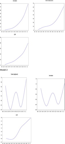
5.3.3. Simulation results of models 1 and 2

The results of the simulations for models 1 and 2 are presented in Figures 15 and 16. Figures 15 and 16 indicate the two models are a good fit because the estimated GDP tracks actual GDP for the entire period. A number of simulations can be carried out by shocking exogenous variables in the macro-econometric model in order to determine the response of the endogenous variable to such shocks.

Figure 15. Actual and estimated GDP (Model 1).

Figure 16. Actual and estimated GDP (Model 2).

5.4. Policy simulations

This section carries out dynamic simulations. This was done by shocking some purely exogenous variables in the macro-econometric model, in order to determine the responsiveness of endogenous variable to the shocked variable. Temporary shocks were carried out in the model. Positive shocks were applied to some exogenous variables from the year 2000 onwards. In line with Akanbi and Du Toit (2011) and Akanbi (2013), the actual values of the selected exogenous variables were increased by 10% during the period 2000–2012. The responses of the variable simulation path were compared to the baseline path (actual values). The results of the responses of endogenous variables to exogenous shocks are presented in Figures 17 and 18. It would be good to impose shocks on many macro-economic variables in the Namibian economy. This means a detailed analysis of the policy implications of various shocks on the Namibian economy. However, this study developed baseline models for further research papers on policy implications of various shocks to the Namibian economy. If a detailed analysis of the policy implications of the various shocks to the Namibian was included, the page and word limitations of the journal would be far exceeded.

Figure 17. Shocks to capital stock.

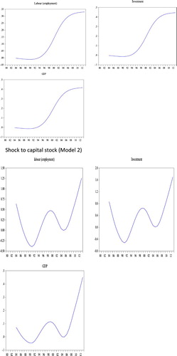
Figure 18. Shocks to Government expenditure.

5.4.1. Shock to capital stock

The results in both Figures 17 and 18 show that macroeconomic variables such as employment, investment and GDP respond positively to a 10% increase in capital stock. The responses are positive for both models 1 and 2. This suggests that an increase in capital stock can be used to expand economic activity and generate employment.

5.4.2. Shock to government expenditure

The results for shocks on government expenditure presented in Figures 17 and 18 indicate that macroeconomic variables such as GDP, employment and investment respond positively to a 10% increase in government expenditure. This suggests that expansionary fiscal policy can be used to expand economic activity and generate the much-needed jobs in Namibia.

6. Conclusion

This paper developed and estimated the supply side macro-econometric model of the Namibian economy using annual data for the period 1980–2013. The model consists of behavioural equations (production, labour, investment, consumption, wages, prices, exports, imports and monetary). The behavioural equations were estimated individually, simulated and were combined and incorporated into a macro-econometric model of the Namibian economy. Endogenous variables in the model were linked by a number of identities and definitions. This was done in order to ensure that the system is fully dynamic. The macro-econometric model was closed using two models. The first model is supply side orientated and it marginalises the demand side. The second model is demand orientated, which marginalises the supply side. These two models were applied to test the hypothesis of structural and demand constraints which inhibit growth and development in Namibia. The complete models were simulated, and the results indicate that the estimated values closely follow or approximate the actual values. This is an indication that the estimated macro-econometric model is a good fit and there is a long-run equilibrium relationship between variables that are included in the macro-econometric model.

The macro-econometric model can be used to apply different policy simulations, in order to determine the optimal economic policy for Namibia. A number of dynamic simulations can be performed by shocking exogenous variables in order to determine the responses of endogenous variables. In order to showcase the dynamics of the Namibian economy, policy simulations of few shocks to the Namibian economy were simulated. Positive shocks were imposed on capital stock and government expenditure. The effect of positive shock on capital stock and government expenditure is beneficial to the economy. Expanding capital stock and expansionary fiscal policy are associated with an increase in economic activity. It would have been appropriate for the study to rely heavily on the policy implications of various shocks to the Namibian economy. However, this was not done, simply because the objective of this paper was to develop baseline models for a series of research papers that can be used to elaborate more on the policy implications of the various shocks to the Namibian economy. A detailed policy analysis is not included in this study because of space limitations.

The structure of the Namibian economy and various simulations from the model suggest that a macro-econometric model which activates the supply side and marginalises the demand side will assist in developing appropriate economic policies. This will help to generate high economic growth and generate the much-need jobs in the country. This suggests that supply side policies are required in Namibia. Policies that aim at increasing economic growth from the supply side are recommended. This will assist in absorbing more people in the economy (generate more jobs) and alleviating poverty.

Disclosure statement

No potential conflict of interest was reported by the author.

References

- Akanbi, OA. 2013. Macroeconomic effects of fiscal policy changes: A case of South Africa. Economic Modelling 35, 771–785. doi: 10.1016/j.econmod.2013.08.039
- Akanbi, OA & Du Toit, CB, 2011. Macroeconometric modelling for the Nigerian economy: A growth-poverty gap analysis. Economic Modelling 28, 335–50. doi: 10.1016/j.econmod.2010.08.015
- Bank of Namibia, 2009. Annual Report. Bank of Namibia, Windhoek.
- Barro, R, 1990. Government spending in a simple model of endogenous growth, Journal of Political Economy 98, S103–25. doi: 10.1086/261726
- Barro, R, 1991. Economic growth in a cross-section of countries. Quarterly Journal of Economics 106(2), 407–43. doi: 10.2307/2937943
- Cobb, CW & Douglass, PH, 1928. A theory of production. American Economic Review 18(1), 139–65.
- Cornwell, R, Leistner, E, & Esterhuysen, E, 1991. Namibia 1990: An African institute country survey. Africa Institute of South Africa, Pretoria.
- Damoense-Azevedo, MY, 2013. Modelling long-run determinants of economic growth for the Mauritian economy. Journal of Developing Areas 47(1), 1–21. doi: 10.1353/jda.2013.0014
- Eita, JH, & Du Toit, CB, 2009. Explaining long-term economic growth in Namibia. South African Journal of Economic and Management Sciences 12(1), 48–62. doi: 10.4102/sajems.v12i1.260
- Engle, R, & Granger, CW, 1987. Cointegration and error correction: Representation, estimation and testing. Econometrica 55, 261–276.
- Hartmann, WP, 1988. The role of mining in the economy of south West Africa/Namibia 1950–1985. Master of Economic Sciences thesis, University of Stellenbosch, Stellenbosch.
- Jorgenson, DW 1963. Capital theory and investment behaviour. American Economic Review 53(2), 247–59.
- Ministry of Labour and Social Welfare, 1997. Namibia labour force survey. Directorate of Labour Market Services, Windhoek.
- Ministry of Labour and Social Welfare, 2000. Namibia labour force survey. Directorate of Labour Market Services, Windhoek.
- Ministry of Labour and Social Welfare, 2002. Namibia labour force survey. Directorate of Labour Market Services, Windhoek.
- Ministry of Labour and Social Welfare, 2004. Namibia labour force survey. Directorate of Labour Market Services, Windhoek.
- Ministry of Labour and Social Welfare, 2008. Namibia labour force survey. Directorate of Labour Market Services, Windhoek.
- Musila, JW, 2002. An econometric model of the Malawian economy. Economic Modelling 19, 295–330. doi: 10.1016/S0264-9993(01)00065-7
- Musila, JW, & Rao, ULG, 2002. A forecasting fodel of the Kenyan economy. Economic Modelling 19, 801–14. doi: 10.1016/S0264-9993(01)00080-3
- National Planning Commission, 2004. Vision 2030. National Planning Commission, Windhoek.