Globalisation, poverty and corruption: Retarding progress in South Africa

ABSTRACT

Poverty and corruption can both immiserate a nation. Globalisation through open trade can potentially increase economic growth, providing employment and increased incomes to the poor. Corruption can dampen or even reduce these positive developments. Although globalisation is considered instrumental in development strategies, theoretically, the impact of globalisation on poverty reduction is ambiguous, an ambiguity that is also reflected in the empirical literature. The corruption-poverty literature clearly reveals that empirical findings on such association are at best heterogeneous. This article examines the effects of globalisation and corruption on poverty using time series data for South Africa for the period 1991–2016. Three indicators of poverty and recently developed measures of globalisation and corruption were employed in the logistic regression model used for estimation. The results confirm that globalisation reduces poverty while corruption intensifies it. The globalisation findings are robust across the different measures of poverty while unidirectional results show corruption increases poverty.

KEYWORDS:

• Corruption
• economic growth
• globalisation
• poverty
• South Africa

JEL CLASSIFICATIONS:

• C5
• C51
• O1
• O11

1. Introduction

South Africa is experiencing state capture and other endemic forms of corruption, low rates of economic growth, high unemployment and high levels of inequality and poverty (Lund & Cois, 2018). After the advent of democracy in 1994, the South African government implemented a range of policies that supported integration into the global economy, where globalisation describes growing interdependence, brought about by greater international trade in goods and services, technologies, and flows of investment, people, and information. The initial Reconstruction and Development Plan (NDP), and subsequent plans provided a framework for economic development to reduce inequality and eliminate poverty. The pro-investment policies that the government rolled out were categorised into two groups. The first focused on creating a favourable investment climate for attracting foreign direct investment (FDI), including trade liberalisation, regionalisation, and industrial development. In the second group were policies that directly targeted FDI, such as exchange rate liberalisation, investment incentives, creation of industrial development zones, special economic zones, and Bilateral Investment Treaties, among other policy initiatives (Magombeyi & Odhiambo, 2018).

South Africa also adopted at least three types of poverty reduction policies. The first entails relief to poor households through social grants, chiefly pensions, child support and disabled persons’ grants. The second focusses on economic empowerment by broadening participation in the economy, including Broad Based Black Economic Empowerment (BBBEE) and land reform. The third comprises increasing resources for social services such as education, health, housing and water. As a result, the poverty headcount decreased until around 2010 but has unfortunately increased since then (Statistics South Africa, 2018). Poverty remains high, with 55.5% of the population living below the upper bound poverty line in 2015, and with sharp differences between population groups, provinces, genders, age cohorts and settlement types (Fransman & Yu, 2018). One possible reason for the recent increase in poverty levels is corruption. While globalisation and other pro-poor initiatives are expected to reduce poverty, corruption is expected to increase it. This study aims to examine if this is the case.

A recent Bureau of Economic Research (2018) report argues that the South African economy performed sub-optimally between 2010 and 2017, and that GDP could have been between 10% and 30% higher; another 500,000–2.5 million more jobs could have been created; and cumulative tax receipts would have been higher by up to $US80 to $US160 billion. Internal causes included widespread policy uncertainty, mismanagement of state resources and state-owned enterprises (SOE) (i.e. corruption), falling business and consumer confidence, widespread drought and various other structural constraints. The Bureau ascribes domestic factors as dominating these outcomes as domestic economic growth tracked the global average quite closely pre-crisis, but began diverging in 2010.

To the best of the authors’ knowledge, three noteworthy studies have so far empirically investigated the effects of globalisation/trade liberalisation on poverty in South Africa. Thurlow (2006) combined a macro-oriented Computable General Equilibrium (CGE) model (to capture globalisation as a macro phenomenon) with a micro-oriented Microsimulation (MS) model (to capture the micro phenomena of poverty and inequality) to assess the effects of trade liberalisation on poverty (measured directly by headcount) and income inequality. Their results indicated that despite rapid trade liberalisation, poverty did not decline. However, inequality deteriorated due to changes in the sectoral structure of production. Based on these findings, the study ruled out any trade-off between trade liberalisation and poverty reduction.

In another study, Hérault (2006) exploited the same macro–micro model but with three indicators of poverty, namely the poverty headcount, poverty gap and income per capita. In this case, the results indicate that trade liberalisation reduced both poverty and income inequality, with a stronger poverty reduction effect. The study attributes this to the contribution of trade liberalisation to the expansion of formal employment through labour relocation both spatially and sectorally.

Erten et al. (2019) examined the effect of trade liberalisation on labour market outcomes, using district-level data for the periods 1994 and 2004. The results indicate that districts which were more exposed to tariff reductions experienced a significant decline in formal and informal employment in the tradable sector, primarily because of a weakening manufacturing sector in the face of strong international competition, especially from China. Displaced workers did not move to other sectors nor did they feel motivated to migrate to better employment opportunities elsewhere. The empirical results are, therefore, mixed with two of these three studies indicating that the effect of trade liberalisation on poverty is ambiguous.

Pillay (2004) undertook a qualitative analysis of the impact of corruption on good governance and the institutional responses to those challenges, which she found to be inadequate and characterised by a lack of public information and a lack of impact by explicit anti-corruption institutions such as the Public Prosecutor, which is the main anti-corruption watchdog. Hoffman (2012) outlined an excellent overview of the state of play of corruption in South Africa focusing on possible legal and policy changes that could be effected to stem the negative impact of corruption on poverty.

Corruption weakens state institutions and gradually erodes an economy’s potential. One measure of the extent of corruption is the Corruption Perceptions Index of Transparency International (2019). This shows South Africa sliding from a ranking of 38 in 2001 to 73 in 2018. The implementation of pro-globalisation and other pro-poor policies and their subsequent effects on poverty are undermined by rising corruption. Therefore, it would be interesting to simultaneously assess the effects of globalisation and corruption on poverty using more recent and robust measures of these variables. A poverty reduction effect of globalisation and a poverty-increasing effect of corruption are the a priori expectations. A set of control variables are included in order to isolate the effects of globalisation and corruption on poverty.

The current study differs significantly from the three quantitative South African studies discussed above, but also from the more general empirical literature. We use more sophisticated measures of both poverty and corruption. Furthermore, a battery of powerful time series econometric techniques are combined with the new variable definitions and data sources. These methodology and data innovations should render better and more policy-relevant findings. This new approach can help address some of the estimation and measurement problems that arise when trying to assess how globalisation and corruption impacts upon poverty.

The aims of the study are two-fold. One, is to examine the impact of globalisation on poverty and two, to assess how corruption affects poverty, both between 1991 and 2016, in South Africa.

The rest of the paper is structured as follows: Section 2 outlines the international literature on globalisation and poverty as well as corruption and poverty. The definitions of poverty and corruption and globalisation, as well as the methodology and data, are outlined in Section 3. Section 4 presents the results, and Section 5 presents some policy implications, with concluding the paper.

2. Literature review

2.1. Globalisation and poverty

The role of globalisation in reducing poverty is contentious, with several issues arising. First, previous studies predominantly focused on growth effects rather than the effects on absolute poverty. Second, most studies ignore the potential endogeneity that might arise from measures of globalisation and economic growth (Bergh & Nilsson, 2014). Third, the multidimensionality of the concept of poverty causes problems: there is still no consensus on how to measure it (Ha & Cain, 2017). Fourth, most previous studies have used trade integration (trade as a share of GDP) as a measure of globalisation, despite the development of more appropriate measures.

Standard trade theory suggests that globalisation (i.e. increased trade) causes a fall in poverty in less developed countries (LDCs) (e.g. Dollar & Kraay, 2004). Some theories focus on the static and dynamic nature of the globalisation-poverty nexus. Static theory such as the Stolper–Samuelson theorem explains the globalisation-poverty association when resources and technology are held constant. It highlights the absolute and comparative advantages of trading countries: countries with absolute advantage, in particular in labour-intensive products, would experience increases in incomes of the poor from trade openness (Krueger, 1983). This argument is corroborated by the neoclassical theory of comparative advantage, which emphasises the transmission channels of labour market mechanisms that affect wages and employment. Under full employment and inter-sectoral labour mobility, trade liberalisation is likely to cause a decline in trading costs that is expected to increase specialisation in the production of goods that require unskilled labour. This should lead to a rise in the wages of the less skilled population, eventually resulting in a reduction in poverty. From a dynamic perspective, economic growth is key to reducing poverty, and trade liberalisation is viewed as stimulating economic growth. Investment incentives, economies of scale, intensified competition, and innovation are the potential positive consequences of trade openness that can reduce poverty (Krueger & Berg, 2003).

Nissanke & Thorbecke (2006) argue that globalisation can also affect poverty indirectly through ‘growth effects’ as well as directly through channels such as changes in relative goods’ prices in favour of (or against) wage goods; changes in relative factor prices induced by trade or factor mobility; the nature of technological progress and the technological diffusion process; volatility and vulnerability; the nature of the worldwide flow of information; and global disinflation. Likewise, institutions can be designed to transmit and amplify the potentially positive benefits of the various mechanisms through which globalisation affects poverty, or alternatively, to block the transmission of those effects.

Agénor (2004) describes several ways in which globalisation can stimulate growth and reduce poverty in the long run. These include standard explanations such as specialisation, scale economies, competition, incentives for macro-economic stability, and innovation. Agénor (2004) further notes that there are several reasons why the short-run effect of globalisation may well be an increase in absolute poverty as a result of a rise in transition costs. With globalisation, capital becomes cheaper, and domestic firms face increased competition, resulting in laid-off workers, which leads to a rise in poverty. Furthermore, openness may lead to the introduction of more advanced technologies, or more capital intensive production, where the full benefits may require more skilled labour than is available.

Salvatore (2004) argued that globalisation increases efficiency, enabling economies of scale, more efficient utilisation of capital and technology, and opportunities for outsourcing domestic resources, while Basu (2006) argued that the prices of goods in poor countries will converge towards the prices in industrialised countries faster than from the latter to the former. As a consequence, wages of unskilled workers from developing countries will lag behind prices temporarily. Skilled workers from developing countries will mostly benefit from globalisation as they can benefit from access to modern technology. Kitson & Michie (1995), on the other hand, show that globalisation may lead to growth divergence through the twin processes of virtuous cycles of trade-induced growth for stronger countries and vicious cycles of trade-induced decline for weaker countries. A similar argument is offered by Kozul-Wright & Rayment (2004:4).

Another source for the adverse effects of globalisation for poor countries may potentially arise from unfavourable terms of trade. Low-income countries often depend on a limited range of mainly primary commodity exports, and regularly experience unfavourable terms of trade, in particular, if the ‘fallacy of composition effect’ is taken into account (Nissanke & Ferrarini, 2001). Integrated multinational oligopolies operating from developed countries may disadvantage a relatively weak country and result in a significantly skewed distribution of the gains from trade (Kaplinsky, 2002).

Liberalisation of trade and investment regimes does not always enable poor countries to grow and improve (Dowrick & DeLong, 2001): openness per se is a necessary but not a sufficient condition to ensure benefits from globalisation also go to the poor. The impact of globalisation/trade openness on poverty reduction is theoretically ambiguous, reflected in the empirical literature as shown in Table 1.

Table 1. Empirical evidence of the relationship between globalisation and poverty reduction.

Author(s)	Data type	Time	Notes on methodology	Results
Trade liberalisation reduces poverty
Desai & Rudra (2018)	Cross-national, time series data for 150 developing countries	2000–10	OLS regression	Countries with trade surpluses in agricultural products because of liberalised trade spend more on social protection by expanding coverage of the extreme poor, eventually reducing poverty. In contrast, developing countries experiencing increased trade in manufacturing experience a decline in social protection coverage, resulting in increased poverty
Olper et al. (2018)	Panel data on child mortality from emerging and developing countries	1960–2010	Addressed potential heterogeneity effects by applying the Synthetic Control Method (SCM)	Trade liberalisation was observed to have significantly reduced poverty for most countries
Ha & Cain (2017)	Panel data on headcount and child mortality rate for over 100 countries	1976–2005	A panel regression technique	Globalisation as measured by trade openness reduces poverty for both indicators
Liyanaarachchi et al. (2016)	Data for Sri Lanka		A macro–micro modelling approach	Trade liberalisation was found to reduce poverty both in the short- and the long-run
Kis-Katos and Sparrow (2015)	Data for 259 districts of Indonesia	1993–2002	Studied the effects of trade liberalisation on poverty through its effect on labour market mechanisms	Reduction in import tariffs on intermediate goods rather than on final inputs drew strong reaction from low-skilled work participation and middle-skilled wages. Intensified competition is a driving force for poverty reduction
Bergh & Nilsson (2014)	Unbalanced panel data (the KOF index of globalisation^a) for 114 countries	1983–2007	Panel regression techniques including fixed effect, a long-run first difference and pooled-OLS regression were applied to address for potential endogeneity of globalisation which had remained unresolved in previous studies	Globalisation reduced absolute poverty and this finding was robust across the different econometric specifications
Tsai & Huang (2007)	Time series data including the income of the bottom quintile of the population and trade as a share of GDP for Taiwan		Regression with cointegration tests	Trade openness alleviated poverty in Taiwan the more open the country’s trade became
The impact of trade liberalisation is either neutral, ambiguous or it does not reduce poverty
Le Goff & Singh (2014)	Cross-country and time-series data on poverty headcount and poverty gap for 30 African countries	1981–2010	Regression analysis using a using the System Generalised Method-of-Moment (GMM) estimator	Trade openness does not increase or decrease poverty for the countries studied, evidence that trade benefits are policy-dependent
Singh & Huang (2011)	Data on financial deepening, headcount poverty, poverty gap, Gini coefficient and income of the poorest quintile for 37 sub-Saharan African countries	1992–2006	Regression using Feasible Generalised Least Squares (FGLS) to address heteroscedasticity	Greater trade openness increased headcount poverty, increased the poverty gap, and caused a decline in the income of the poorest quintile
Attanasio et al. (2004)	Tariff reductions and wage distribution in Colombia	1980s and 1990s	Regression analysis	Tariff reductions caused a rise in unemployment in traded-good sectors
Goldberg & Pavcnik (2003)	Trade and employment data from Brazil and Colombia	1980s and 1990s	Regression analysis	In an environment of more intense competition, firms may reduce their costs by substituting for temporary workers. This might cause a rise in poverty
Nissanke & Thorbecke (2010)	A review of nine empirical papers on globalisation and inequality and poverty in Latin America		Review	The impact of globalisation on poverty and inequality is extremely context specific

^aThe KOF Index of Globalisation is an index of the degree of globalisation of 122 countries, conceived by the Konjunkturforschungsstelle of ETH Zurich, in Switzerland (Swiss Economic Institute, 2018).

This theoretical and empirical discussion leads to a number of conclusions. First, the issue has not been exhausted. Second, the poverty effects of globalisation are mixed, conditional and context specific. Third, there is little consensus on what indicators of poverty and globalisation should be used in trying to ascribe causality. The multidimensionality of the concept of poverty makes such an association even more confusing. Fourth, most studies do not resolve the potential endogeneity problem: globalisation can be both a cause and an effect of poverty. Fifth, panel studies dominate the empirical literature although country-specific characteristics matter. Sixth, most studies used trade integration as a measure of globalisation/trade openness and not more appropriate measures of globalisation which have recently been developed. Finally, the empirical evidence is inconclusive. These arguments justify further investigation of such an association and South Africa is an ideal candidate for such an empirical exercise.

2.2. Corruption and poverty

Despite a growing body of literature, the question of whether corruption ‘greases’ or ‘sands’ the wheels of development is still unresolved. One reason for this empirical ‘impasse’ is a fundamental problem with the concept of corruption itself. It is a multidimensional concept. The empirical stand-off is further exasperated by data reliability. Since corruption is, by its nature, difficult to measure, high-quality data from developing countries are scarce.

Corruption could be a hurdle to economic development and thereby intensify poverty through a number of channels. It weakens national institutions and increases economic inefficiencies (Gupta et al., 2002), reduces economic growth (Ugur, 2014), hampers the productivity of the public sector (Tanzi, 1995), reduces private sector investment (Cieślik & Goczek, 2018), reduces FDI in developing countries (Gossel, 2018), increases inflation (Ben Ali & Sassi, 2016), causes a decline in personal incomes (Husted, 1999), intensifies income inequality and poverty (Gupta et al., 2002), lowers expenditure on health and education (Ben Ali et al., 2016) and more generally hampers economic development (Poveda et al., 2019). Corruption is economically damaging as resources are transferred to unproductive activities (Cieślik & Goczek, 2018). Méon & Sekkat (2005) found that corruption decreases economic growth more in nations with weak rule of law and inefficient government.

The other side of the debate maintains that corruption can under certain conditions, be beneficial as it can ‘grease the wheels’ of commerce by bypassing public sector rules and ‘impediments’. It can help firms deal with complex government regulations, handle bureaucratic tangles, constrain the ‘leapfrogging’ nature of government, and stimulate innovation (see, e.g. Huntington, 1968). Dreher & Gassebner (2013) found that corruption helps new firms overcome bureaucratic obstacles (also see Bologna & Ross, 2015).

The empirical literature studying the direct effect of corruption on poverty is limited. Justesen & Bjørnskov (2014) used survey data from Afrobarometer to study the effect of corruption on poverty, using a multilevel regression for 18 African countries. Poor people suffer more from corruption as they are more exposed to paying bribes for basic services. This was corroborated by Adebayo (2013) who found that corruption intensified poverty in Nigeria. Rahayu & Widodo (2012) analysed the empirical relationship between corruption and poverty using data for a panel of nine ASEAN countries between 2005 and 2009. They applied a two-step Generalised Method of Moments (GMM) model and found that corruption affects poverty. Also, corruption unidirectionally causes poverty.

Negin et al. (2010) assessed the impact of corruption using panel data for 97 developing countries using the corruption perception index from Transparency International and the Human Development Index to measure poverty. They found a bi-directional causality between corruption and poverty.

Dincer & Gunalp (2008) analysed the impact of corruption on income inequality and poverty in the United States using both time series and cross sectional data, finding that an increase in corruption was accompanied by a rise in inequality and poverty. The results were robust across different measures of variables and different econometric specifications.

N’zue & N’guessan (2006) examined the empirical link among corruption, poverty and growth for a panel of 18 African countries for the period 1996–2001. Using fixed and random effect models, they found no causal association between corruption and poverty.

This overview of the corruption-poverty literature shows that empirical findings are at best heterogeneous. Therefore, a fresh time series investigation into the empirical link in the context of South Africa, where both poverty and corruption are prevalent, seems timely.

3. Methodology

3.1. Variable description and data

Poverty is a multidimensional and multifaceted concept which is difficult to measure, and the methodological debate continues unabated (Ravallion, 2003; Ha & Cain, 2017). The simplest and most direct measure of absolute poverty the poverty headcount, and the preferred measure in the literature is the poverty headcount index, set by the World Bank as a percentage of the population of a country living at below $1.90 per person per day, adjusted by the 2011 purchasing power parity (PPP) (World Bank, 2015). However, it has been criticised for being too simplistic, which can lead to erroneous policy prescriptions (World Bank, 2015). Nonetheless, Ravallion (2003) argues that the World Bank's measure of absolute poverty remains the best available.

However, a composite index should be considered because of the multidimensional nature of poverty. There are also different measures using this approach which focus on the non-monetary aspects of poverty (Liyanaarachchi et al., 2016). For robustness purposes, two other widely accepted indirect measures of poverty, namely the infant mortality rate (MR) (defined as the number of deaths per 1000 live births of children under one year of age) and life expectancy at birth (LE) (defined as an estimate of the average age that members of a particular population group will reach at death), are used here, as they better reflect the actual living standard of poor people (Ghobarah et al., 2004). Olper et al. (2018) and Ha & Cain (2017) have undertaken studies which use combinations of the poverty headcount and/or infant mortality and life expectancy. Therefore, this study includes three different indicators of poverty as the dependent variable; a direct measure – headcount or absolute poverty and two indirect measures – infant mortality rate and life expectancy. Those three indicators are used independently for estimation purposes and to cross-check the estimates obtained.

The core independent variables are globalisation and corruption.

Most studies in the literature use trade integration (trade as a share of GDP) as a rather simplistic measure of globalisation. However, more appropriate methods exist. These include the KOF index which measures globalisation across economic, social and political dimensions (Dreher, 2006). The key advantage of this index is that it allows a separate analysis of economic flows and trade policies. Bergh & Nilsson (2014) conducted one of the first studies of the globalisation-poverty nexus to use the index.

The concept of corruption is also multidimensional, further exacerbated by poor data reliability, since corruption is, by its nature, difficult to observe (Klitgaard, 2017). Different measures of the extent of corruption exist, including:

• The Corruption Perceptions Index of Transparency International. However, Hessami (2014) argues that year-to-year comparisons are unreliable because it is not a composite index.

• The International Country Risk Guide (ICRG) rating from the PRS Group which comprises 22 variables in 3 subcategories of risk: political, financial and economic. It is considered superior to other potential measures.

• The World Bank World Governance Indicators, which are the most commonly used measure. It comprises six indicators, including control of corruption and the rule of law.

This latter measure was selected for estimation purposes in this study, based on ease of data availability (World Bank, 2018).

A set of control variables is also considered in the model, including: (i) economic growth, proxied by real GDP per capita (GDPPC) and measured at constant US$2005, (ii) foreign direct investment (FDI) as a share of GDP, (iii) financial development (FD) measured by domestic credit to the private sector as a share of GDP, (iv) number of Internet users per 100 people (INT), (v) number of mobile subscriptions per 100 people (MOB), (vi) education (EDU) measured by secondary school enrolments and (vii) institutional quality (INQ) proxied by the rule of law. Data for the control of corruption (CPT) and compliance with the rule of law were obtained from the World Governance Indicators (WGI) database (World Bank, 2018). Data for all other variables were obtained from the World Development Indicators (WDI) database (World Bank, 2017).

Variables HC, MR, LE, GDPPC, GLO, EDU and MOB underwent logarithmic transformation to reduce heteroscedasticity. A summary of variable description, sources and statistics are provided in Table 2.

Table 2. Data sources and summary statistics.

Source	Definition	Variables	Obs.	Mean	Std. dev.	Min	Max
WDI (2017)	Logarithm of poverty headcount ratio at $1.90 a day (2011 PPP) (% of population)	Log poverty headcount	27	4.1103	0.0214	4.0634	4.1494
	Logarithm of mortality rate, infant (per 1000 live births)	Log mortality Rate	27	3.7521	0.1130	3.5322	3.8979
	Logarithm of life expectancy	Log life expectancy	27	4.0543	0.0626	3.9620	4.1336
	Logarithm of GDP per capita (constant 2010, US$)	Log GDPPC	27	8.4092	0.3519	7.8337	8.9945
	Percentage of population using the Internet	Internet use	27	14.8617	18.3919	0.0133	54.0000
	Logarithm of financial development	Log FD	27	5.9328	0.2343	5.3102	6.2898
	Foreign direct investment	FDI	27	1.3003	1.3345	0.0025	5.9789
	Percentage of mobile cellular subscriptions	Log mobile	27	3.1581	1.7655	0.2558	5.1030
	Secondary school enrolment	Log education	27	4.4839	0.0809	4.2414	4.5933
KOF Swiss Economic Institute (2018)	Globalisation index	Log GLO	27	3.8491	0.1325	3.5812	3.9857
WGI (2018)	Control of corruption	Corruption	27	3.3336	1.0787	2.0000	5.0000
	Rule of law	Institutional quality	27	2.4984	0.6562	1.0000	4.0000

Source: Authors’ own calculations.

3.2. Models

Three regression models are used to investigate the impacts of globalisation and corruption on the dependent variable, poverty, measured using three different specifications. Model 1 investigates the impact using lnHC (headcount poverty), Model 2 uses lnMR (infant mortality rate), while Model 3 captures the dynamic impact lnLE (life expectancy). The models are specified in Equations (1) through (3).(1) $\begin{array}{rl}\mathrm{M}\mathrm{o}\mathrm{d}\mathrm{e}\mathrm{l}1:\mathrm{l}\mathrm{n}\mathrm{H}\mathrm{C}=& {\text{β}}_0+{\text{β}}_1\mathrm{l}\mathrm{n}\mathrm{G}\mathrm{L}\mathrm{O}+{\text{β}}_2\mathrm{C}\mathrm{P}\mathrm{T}{\text{β}}_1+{\propto }_1\mathrm{l}\mathrm{n}\mathrm{G}\mathrm{D}\mathrm{P}\mathrm{P}\mathrm{C}+{\propto }_2\mathrm{l}\mathrm{n}\mathrm{F}\mathrm{D}+{\propto }_3\mathrm{F}\mathrm{D}\mathrm{I}\\ & +{\propto }_4\mathrm{N}\mathrm{E}\mathrm{T}+{\propto }_5\mathrm{l}\mathrm{n}\mathrm{M}\mathrm{O}\mathrm{B}+{\propto }_6\mathrm{I}\mathrm{N}\mathrm{Q}+{\propto }_7\mathrm{l}\mathrm{n}\mathrm{E}\mathrm{D}+{\epsilon }_t\end{array}$(1) (2) $\begin{array}{rl}\mathrm{M}\mathrm{o}\mathrm{d}\mathrm{e}\mathrm{l}2:\mathrm{l}\mathrm{n}\mathrm{M}\mathrm{R}=& {\text{β}}_0+{\text{β}}_1\mathrm{l}\mathrm{n}\mathrm{G}\mathrm{L}\mathrm{O}+{\text{β}}_2\mathrm{C}\mathrm{P}\mathrm{T}{\text{β}}_1+{\mathrm{\Phi }}_1\mathrm{l}\mathrm{n}\mathrm{G}\mathrm{D}\mathrm{P}\mathrm{P}\mathrm{C}+{\mathrm{\Phi }}_2\mathrm{l}\mathrm{n}\mathrm{F}\mathrm{D}+{\mathrm{\Phi }}_3\mathrm{F}\mathrm{D}\mathrm{I}\\ & +{\mathrm{\Phi }}_4\mathrm{N}\mathrm{E}\mathrm{T}+{\mathrm{\Phi }}_5\mathrm{l}\mathrm{n}\mathrm{M}\mathrm{O}\mathrm{B}+{\mathrm{\Phi }}_6\mathrm{I}\mathrm{N}\mathrm{Q}+{\mathrm{\Phi }}_7\mathrm{l}\mathrm{n}\mathrm{E}\mathrm{D}+{\epsilon }_t\end{array}$(2) (3) $\begin{array}{rl}\mathrm{M}\mathrm{o}\mathrm{d}\mathrm{e}\mathrm{l}3:\mathrm{l}\mathrm{n}\mathrm{L}\mathrm{E}=& {\text{β}}_0+{\text{β}}_1\mathrm{l}\mathrm{n}\mathrm{G}\mathrm{L}\mathrm{O}+{\text{β}}_2\mathrm{C}\mathrm{P}\mathrm{T}{\text{β}}_1+{\mathrm{\Omega }}_1\mathrm{l}\mathrm{n}\mathrm{G}\mathrm{D}\mathrm{P}\mathrm{P}\mathrm{C}+{\mathrm{\Omega }}_2\mathrm{l}\mathrm{n}\mathrm{F}\mathrm{D}+{\mathrm{\Omega }}_3\mathrm{F}\mathrm{D}\mathrm{I}\\ & +{\mathrm{\Omega }}_4\mathrm{N}\mathrm{E}\mathrm{T}+{\mathrm{\Omega }}_5\mathrm{l}\mathrm{n}\mathrm{M}\mathrm{O}\mathrm{B}+{\mathrm{\Omega }}_6\mathrm{I}\mathrm{N}\mathrm{Q}+{\mathrm{\Omega }}_7\mathrm{l}\mathrm{n}\mathrm{E}\mathrm{D}+{\epsilon }_t\end{array}$(3) where β₀ is a constant, the βs are the coefficients of the two core independent variables, ∝s, ɸs and Ωs are the coefficients of the seven control variables and ε_t is the stochastic error term.

3.3. Estimation procedures

3.3.1. Unit root tests

Taking into account the presence of structural break in data, the Zivot & Andrews (1992) unit root test was employed, which allows a single structural break point in the data. If the series is viewed as X, the structural tests take the form:(4) $\mathrm{\Delta }{X}_t=\mathrm{\Omega }+\mathrm{\Omega }{X}_{t-1}+ct+d{D}_t+dD{T}_t+\sum _{j=1}^k{d}_j\mathrm{\Delta }{X}_{t-j}+{\epsilon }_t$(4) (5) $\mathrm{\Delta }{X}_t=a+a{X}_{t-1}+bT+c{D}_t+\sum _{j=1}^k{d}_j\mathrm{\Delta }{X}_{t-j}+{\epsilon }_t$(5) (6) $\mathrm{\Delta }{X}_t=\text{β}+\text{β}{X}_{t-1}+ct+bD{T}_t+\sum _{j=1}^k{d}_j\mathrm{\Delta }{X}_{t-j}+{\epsilon }_t$(6) (7) $\mathrm{\Delta }{X}_t=\gamma +\gamma X_{t-1}+ct+dD{T}_t+\sum _{j=1}^k{d}_j\mathrm{\Delta }{X}_{t-j}+{\epsilon }_t$(7) where D is a dummy variable and shows the mean shift at each point, and DT_t is a trend shift variable. The null hypothesis c = 0 supports the presence of unit root in the absence of structural break hypothesis against the alternative that the series is trend stationary with an unknown time break. Then, this unit root test selects that time break which reduces the one-sided t-statistic to test c(= c − 1) = 1.

3.4. Cointegration tests

3.4.1. ARDL bounds testing approach to cointegration

Conventional cointegration techniques suffer weak findings because of the presence of structural breaks in macro-economic dynamics (Lutkepohl, 2006), hence an econometric technique known as Autoregressive Distributed Lag (ARDL) bounds testing, developed by Pesaran et al. (2001), is applied here to assess the cointegrating relationship between the variables. There are three different possibilities or outcomes in deciding about the significance of the bounds testing approach to cointegration. For example, there could be cointegration, no-cointegration or indecisive, depending on the comparison of the calculated F and the critical bound values.

The ARDL bounds testing approach was selected on a number of grounds. First, it involves the use of a single reduced form equation rather than a system of equations (see Duasa, 2007). Second, it does not require all variables to be integrated of the same order. It can be applied even when variables are integrated of order 1 [I (1)], or of order 0 [I (0)] or fractionally integrated (Pesaran et al., 2001). Then, this method can also be applied to a small sample size study as in this study (Pesaran et al., 2001). Third, it simultaneously estimates the short-run dynamics and the long-run equilibrium within a dynamic unrestricted error correction model (UCEM) through a simple linear transformation of variables. Fourth, it estimates the short and long-run components, potentially removing the problems of bias resulting from omitted variables and autocorrelation. In addition, the technique generally provides unbiased estimates for the long-run model and valid t-statistics even when the model is plagued with the problem of endogeneity (Harris & Sollis, 2003).

The empirical formulation of ARDL equations for the three models are specified as follows:(8) $\begin{array}{rl}\mathrm{\Delta }\mathrm{l}\mathrm{n}\mathrm{H}{\mathrm{C}}_t=& {\text{β}}_0+{\text{β}}_{1}T+{\text{β}}_{2}D+{\text{β}}_3\mathrm{l}\mathrm{n}\mathrm{H}{\mathrm{C}}_{t-1}+{\text{β}}_4\mathrm{l}\mathrm{n}\mathrm{G}\mathrm{L}\mathrm{O}+{\text{β}}_5\mathrm{C}\mathrm{P}\mathrm{T}+{\propto }_1\mathrm{l}\mathrm{n}\mathrm{G}\mathrm{D}\mathrm{P}\mathrm{P}\mathrm{C}\\ & +{\propto }_2\mathrm{l}\mathrm{n}\mathrm{F}\mathrm{D}+{\propto }_3\mathrm{F}\mathrm{D}\mathrm{I}+{\propto }_4\mathrm{N}\mathrm{E}\mathrm{T}+{\propto }_5\mathrm{l}\mathrm{n}\mathrm{M}\mathrm{O}\mathrm{B}+{\propto }_6\mathrm{I}\mathrm{N}\mathrm{Q}+{\propto }_7\mathrm{l}\mathrm{n}\mathrm{E}\mathrm{D}\\ & +\sum _{i=0}^P{\text{β}}_6\mathrm{\Delta }\mathrm{l}\mathrm{n}\mathrm{H}{\mathrm{C}}_{t-j}+\sum _{j=0}^q{\text{β}}_7\mathrm{\Delta }\mathrm{l}\mathrm{n}\mathrm{G}\mathrm{L}{\mathrm{O}}_{t-j}+\sum _{k=0}^r{\text{β}}_8\mathrm{\Delta }\mathrm{l}\mathrm{n}\mathrm{C}\mathrm{P}{\mathrm{T}}_{t-j}\\ & +\sum _{l=0}^s{\propto }_8\mathrm{\Delta }\mathrm{l}\mathrm{n}\mathrm{G}\mathrm{D}\mathrm{P}\mathrm{P}{\mathrm{C}}_{t-j}+\sum _{m=0}^t{\propto }_9\mathrm{\Delta }\mathrm{l}\mathrm{n}\mathrm{F}{\mathrm{D}}_{t-j}+\sum _{n=0}^u{\propto }_{10}\mathrm{\Delta }\mathrm{l}\mathrm{n}\mathrm{F}\mathrm{D}{\mathrm{I}}_{t-j}\\ & +\sum _{o=0}^v{\propto }_{11}\mathrm{\Delta }\mathrm{N}\mathrm{E}{\mathrm{T}}_{t-j}+\sum _{p=0}^w{\propto }_{12}\mathrm{\Delta }\mathrm{l}\mathrm{n}\mathrm{M}\mathrm{O}{\mathrm{B}}_{t-j}\\ & +\sum _{q=0}^x{\propto }_{13}\mathrm{\Delta }\mathrm{l}\mathrm{n}\mathrm{E}{\mathrm{D}}_{t-k}+{\epsilon }_t\end{array}$(8) (9) $\begin{array}{rl}\mathrm{\Delta }\mathrm{l}\mathrm{n}\mathrm{M}{\mathrm{R}}_t=& {\text{β}}_0+{\text{β}}_{1}T+{\text{β}}_{2}D+{\text{β}}_3\mathrm{l}\mathrm{n}\mathrm{H}{\mathrm{C}}_{t-1}+{\text{β}}_4\mathrm{l}\mathrm{n}\mathrm{G}\mathrm{L}\mathrm{O}+{\text{β}}_5\mathrm{C}\mathrm{P}\mathrm{T}+{\propto }_1\mathrm{l}\mathrm{n}\mathrm{G}\mathrm{D}\mathrm{P}\mathrm{P}\mathrm{C}\\ & +{\propto }_2\mathrm{l}\mathrm{n}\mathrm{F}\mathrm{D}+{\propto }_3\mathrm{F}\mathrm{D}\mathrm{I}+{\propto }_4\mathrm{N}\mathrm{E}\mathrm{T}+{\propto }_5\mathrm{l}\mathrm{n}\mathrm{M}\mathrm{O}\mathrm{B}+{\propto }_6\mathrm{I}\mathrm{N}\mathrm{Q}+{\propto }_7\mathrm{l}\mathrm{n}\mathrm{E}\mathrm{D}\\ & +\sum _{i=0}^P{\text{β}}_6\mathrm{\Delta }\mathrm{l}\mathrm{n}\mathrm{H}{\mathrm{C}}_{t-j}+\sum _{j=0}^q{\text{β}}_7\mathrm{\Delta }\mathrm{l}\mathrm{n}\mathrm{G}\mathrm{L}{\mathrm{O}}_{t-j}+\sum _{k=0}^r{\text{β}}_8\mathrm{\Delta }\mathrm{l}\mathrm{n}\mathrm{C}\mathrm{P}{\mathrm{T}}_{t-j}\\ & +\sum _{l=0}^s{\propto }_8\mathrm{\Delta }\mathrm{l}\mathrm{n}\mathrm{G}\mathrm{D}\mathrm{P}\mathrm{P}{\mathrm{C}}_{t_{-}j}+\sum _{m=0}^t{\propto }_9\mathrm{\Delta }\mathrm{l}\mathrm{n}\mathrm{F}{\mathrm{D}}_{t-j}\\ & +\sum _{n=0}^u{\propto }_{10}\mathrm{\Delta }\mathrm{l}\mathrm{n}\mathrm{F}\mathrm{D}{\mathrm{I}}_{t-j}+\sum _{o=0}^v{\propto }_{11}\mathrm{\Delta }\mathrm{N}\mathrm{E}{\mathrm{T}}_{t-j}+\sum _{p=0}^w{\propto }_{12}\mathrm{\Delta }\mathrm{l}\mathrm{n}\mathrm{M}\mathrm{O}{\mathrm{B}}_{t-j}\\ & +\sum _{q=0}^x{\propto }_{13}\mathrm{\Delta }\mathrm{l}\mathrm{n}\mathrm{E}{\mathrm{D}}_{t-k}+{\epsilon }_t\end{array}$(9) (10) $\begin{array}{rl}\mathrm{\Delta }\mathrm{l}\mathrm{n}\mathrm{L}{\mathrm{E}}_t=& {\text{β}}_0+{\text{β}}_{1}T+{\text{β}}_{2}D+{\text{β}}_3\mathrm{l}\mathrm{n}\mathrm{H}{\mathrm{C}}_{t-1}+{\text{β}}_4\mathrm{l}\mathrm{n}\mathrm{G}\mathrm{L}\mathrm{O}+{\text{β}}_5\mathrm{C}\mathrm{P}\mathrm{T}+{\propto }_1\mathrm{l}\mathrm{n}\mathrm{G}\mathrm{D}\mathrm{P}\mathrm{P}\mathrm{C}\\ & +{\propto }_2\mathrm{l}\mathrm{n}\mathrm{F}\mathrm{D}+{\propto }_3\mathrm{F}\mathrm{D}\mathrm{I}+{\propto }_4\mathrm{N}\mathrm{E}\mathrm{T}+{\propto }_5\mathrm{l}\mathrm{n}\mathrm{M}\mathrm{O}\mathrm{B}+{\propto }_6\mathrm{I}\mathrm{N}\mathrm{Q}+{\propto }_7\mathrm{l}\mathrm{n}\mathrm{E}\mathrm{D}\\ & +\sum _{i=0}^P{\text{β}}_6\mathrm{\Delta }\mathrm{l}\mathrm{n}\mathrm{H}{\mathrm{C}}_{t-j}+\sum _{j=0}^q{\text{β}}_7\mathrm{\Delta }\mathrm{l}\mathrm{n}\mathrm{G}\mathrm{L}{\mathrm{O}}_{t-j}+\sum _{k=0}^r{\text{β}}_8\mathrm{\Delta }\mathrm{l}\mathrm{n}\mathrm{C}\mathrm{P}{\mathrm{T}}_{t-j}\\ & +\sum _{l=0}^s{\propto }_8\mathrm{\Delta }\mathrm{l}\mathrm{n}\mathrm{G}\mathrm{D}\mathrm{P}\mathrm{P}{\mathrm{C}}_{t-j}+\sum _{m=0}^t{\propto }_9\mathrm{\Delta }\mathrm{l}\mathrm{n}\mathrm{F}{\mathrm{D}}_{t-j}+\sum _{n=0}^u{\propto }_{10}\mathrm{\Delta }\mathrm{l}\mathrm{n}\mathrm{F}\mathrm{D}{\mathrm{I}}_{t-j}\\ & +\sum _{o=0}^v{\propto }_{11}\mathrm{\Delta }\mathrm{N}\mathrm{E}{\mathrm{T}}_{t-j}+\sum _{p=0}^w{\propto }_{12}\mathrm{\Delta }\mathrm{l}\mathrm{n}\mathrm{M}\mathrm{O}{\mathrm{B}}_{t-j}+\sum _{q=0}^x{\propto }_{13}\mathrm{\Delta }\mathrm{l}\mathrm{n}\mathrm{E}{\mathrm{D}}_{t-k}+{\epsilon }_t\end{array}$(10) where Δ is the difference operator. T and D denote time trend and dummy variable, respectively. The dummy variable is included in the equations of all three models to capture the structural break arising from the series. ε_t is the disturbance term.

To examine the cointegrating relationship, a Wald Test or the F-test for the joint significance of the coefficients of the lagged variables is applied with the null hypothesis, H₀: β₃ = β₄ = β₅ indicating no cointegration against the alternative hypothesis of the existence of cointegration between variables. F-statistics are computed to compare the upper and lower bounds with critical values provided by Pesaran et al. (2001).

3.4.2. Toda Yamamoto causality test

Next, this study examines the causal direction among key variables. Since the variables are integrated with mixed order of integration, a traditional Granger causality test (Granger, 1969) is not ideal as it is sensitive to the order of integration among variables. Therefore, TY causality test was conducted (for detailed mathematical derivations, see Toda & Yamamoto, 1995).

3.4.3. Variance decomposition analysis

Since the ARDL estimates do not provide any inference about the relationship beyond the sample period covered in the study, the variance decomposition method was employed to assess the percentage contribution of each independent variable to the h-step ahead forecast error variance of the dependent variable (Pesaran & Shin, 1999). This produces more reliable results than other traditional approaches (Engle & Granger, 1987; Ibrahim, 2005).

4. Results

Table 3 presents Variance Inflation Factor (VIF) results which indicate that none of the three models suffers from a high level of multicollinearity since the VIF values are well below five. Table 4 displays the results of the Zivot & Andrews (1992) structural break unit root test which shows that poverty measured by poverty headcount and life expectancy, Internet use, log FD and corruption are stationary at levels, while other variables are found stationary at first difference, in the presence of a structural break. Most of the series are characterised by structural breaks during the period from late 1990s and throughout 2000s.

Table 3. Variance inflation factor (VIF) results.

Variable	VIF	1/VIF
lnGLO	1.84	0.542067
COR	2.87	0.347991
INT	2.14	0.467111
INQ	1.88	0.531434
lnFD	2.92	0.342795
lnGDPPC	1.56	0.642542
lnMOB	1.43	0.698292
LnEDU	1.17	0.853386
FDI	1.08	0.928105
Mean VIF	1.88

Table 4. Zivot and Andrews unit root test results.

Variables	Levels			1st Difference
	T-statistic	Time break	Decision	T-statistic	Time break	Decision
lnHC	−5.852*	2008	Stationary
lnMR	−2.800	2009	Unit root	−7.748*	2010	Stationary
lnLE	−24.639*	2008	Stationary
lnGLO	−4.587	1997	Unit root	−6.016*	2003	Stationary
COR	−7.056*	1998	Stationary
lnGDPPC	−3.303	2003	Unit root	−6.107*	2003	Stationary
lnFD	−5.495*	2005	Stationary
FDI	−5.194	2001	Unit root	−6.912*	2007	Stationary
INT	−17.799*	2010	Stationary
lnEDU	−4.576	2000	Unit root	−8.707*	2002	Stationary
INQ	−5.208	1998	Unit root	−5.535*	1996	Stationary
lnMOB	−3.169	1997	Unit root	−5.970*	1999	Stationary

*Represents significance at 1% level.

Table 5 reports results from ARDL cointegration for all three models. The F-statistics for Models 1, 2 and 3 are 13.254, 17.879 and 11.7502 respectively. The calculated F-statistics are compared to the Pesaran et al. (2001) critical values. In all models, the calculated F-statistic is greater than the upper critical bounds (UCB) values which imply a cointegrating relationship among the variables. After confirming the long-run relationship in Models 1–3, the ARDL procedure is used in the estimation of the three models. To proceed with the estimation, the optimal lag length is selected based on Bayesian Information Criteria (BIC), which produced more parsimonious results than the Akaike Information Criteria (AIC)-based models. The optimal lag length selected for Model 1 is ARDL (2, 3, 3, 1, 2, 2, 3, 1, 1); for Model 2 it is ARDL (2, 1, 2, 2, 3, 0, 1, 2, 3); and for Model 3 it is ARDL (2, 1, 3, 1, 0, 2, 4, 3, 1).

Table 5. ARDL cointegration results and critical values.

Models	Independent variables	Function		F-statistic		Cointegration status
1	lnHC	F(lnGLO, lnCOR, lnGDPPC, INT, lnFD, FDI, lnEDU, INT, lnMOB, INQ)		13.254***		Cointegrated
2	lnMR	F(lnGLO, lnCOR, lnGDPPC, INT, lnFD, FDI, lnEDU, INT, lnMOB, INQ)		17.879***		Cointegrated
3	LnLE	F(lnGLO, lnCOR, lnGDPPC, INT, lnFD, FDI, lnEDU, INT, lnMOB, INQ)		11.502***		Cointegrated
Asymptotic Critical Values (unrestricted intercept and no trend)
Pesaran et al. (2001:300) critical values (Table CI(iii) Case III)		10%		5%		1%
		I(0)	I(1)	I(0)	I(1)	I(0)	I(1)
		2.62	3.35	2.26	3.79	3.41	4.68

Note: *, ** and *** denote statistical significance at 10%, 5% and 1% levels respectively.

The long-run and short-run coefficients obtained from the estimations of Models 1–3 are presented in Tables 6–8, respectively. The regression results for Model 1 presented in Table 6 shows that globalisation reduces poverty as measured by all three indicators (poverty headcount, infant mortality rate and life expectancy) in the long run. A 1% increase in globalisation reduces poverty headcount and the infant mortality rate by 0.08% (statistically significant) and 1.68%, respectively. Also, a 1% increase in globalisation pushes life expectancy up by 1.54%. The long-run coefficients suggest that globalisation has a stronger impact on the indirect measures of poverty than on its direct measure (poverty headcount). In the short run, globalisation reduces both poverty headcount (statistically significant) and infant mortality rate. However, its effect in the short run on life expectancy is negative and statistically insignificant.

Table 6. ARDL analysis results (lnHC): long and short run.

Dependent variable = lnHC
Variables	Coefficient	Standard error	T-statistics[Prob]
Long-run analysis
Constant	0.742	0.421	1.761[0.009]
GLO	−0.084	0.038	2.214[0.069]
COR	0.041	0.004	9.582[0.000]
Control variables
lnGDPPC	0.159	0.018	9.032[0.000]
INQ	−0.045	0.007	−6.729[0.001]
lnFD	−0.163	0.011	−14.932[0.000]
FDI	0.076	0.010	7.796[0.000]
lnEDU	−0.002	0.001	−2.924[0.027]
ICT	−0.316	0.032	−9.814[0.000]
INT	0.001	0.000	3.275[0.017]
lnMOB	−0.050	0.014	−3.549[0.012]
R^2	0.9876
Short-run analysis
Constant
ΔGLO	−0.062	0.010	−6.186[0.001]
ΔCOR	0.027	0.002	23.008[0.000]
Control variables
ΔlnGDPPC	0.047	0.003	14.545[0.000]
ΔINQ	−0.036	0.005	−6.6704[0.000]
ΔlnFD	0.076	0.003	23.934[0.000]
ΔFDI	−0.002	0.000	−16.195[0.000]
ΔlnEDU	−0.030	0.008	−3.640[0.011]
ICT
ΔINT	0.001	0.000	14.172[0.000]
ΔlnMOB	−0.064	0.003	−24.828[0.000]
ECMt−1	−0.071	0.002	−31.425[0.000]
R^2	0.986
F-statistic	51.673[0.000]
D. W	2.304
Short-run diagnostic tests
Test	F-statistic	Prob. value
χ^2SERIAL	0.1677	0.089
χ^2ARCH	3.3762	0.079
χ^2RAMSEY	2.4162	0.046

Table 7. ARDL analysis results (lnMR): long and short run.

Dependent variable = lnMR
Variables	Coefficient	Standard error	T-statistics[Prob]
Long-run analysis
Constant	1.7621	0.81890	2.1519[0.057]
GLO	−1.6849	0.68421	2.4625[0.030]
COR	0.0079	0.022052	−0.35998[0.025]
Control variables
lnGDPPC	0.1623	0.15948	1.0182[0.329]
INQ	0.1763	0.066281	2.6602[0.021]
lnFD	−0.0027	0.012912	−0.21337[0.835]
FDI	−0.0015	0.008867	−0.16921[0.868]
lnEDU	1.4077	0.84664	1.6626[0.122]
ICT
INT	0.0017	0.001049	1.6276[0.130]
lnMOB	0.1209	0.12662	0.95529[0.358]
R^2	0.9035
Short-run analysis
Constant	1.7621	0.81890	2.1519[0.057]
ΔGLO	−1.3963	0.44861	3.1125[0.007]
ΔCOR	−0.0664	0.048106	−1.3811[0.187]
Control variables
ΔlnGDPPC	0.13457	0.12647	1.0641[0.304]
ΔlnFD	−0.7024	0.12361	−5.6824[0.000]
ΔFDI	−0.0012	0.007316	−0.16995[0.867]
ΔINQ	0.1461	0.043157	3.3857[0.004]
ΔlnEDU	0.3388	0.37141	0.91231[0.376]
ICT
ΔINT	0.0014	0.8889E−3	1.5928[0.132]
ΔlnMOB	0.1002	0.10193	0.98337[0.341]
ECMt−1	−0.8287	0.15597	−5.3132[0.000]
R^2	0.9054
F-statistic	12.7752[0.000]
D. W	2.6471
Short-run diagnostic tests
Test	F-statistic	Prob. value
χ^2SERIAL	4.2525	0.064
χ^2ARCH	0.16036	0.003
χ^2RAMSEY	2.0876	0.076

Table 8. ARDL analysis results (lnLE): long and short run.

Dependent variable = lnLE
Variables	Coefficient	Standard error	T-statistics[Prob]
Long-run analysis
Constant	3.4733	0.37086	9.3657[0.000]
GLO	1.5448	0.77058	2.0047[0.080]
COR	−0.0073	0.038828	−0.18851[0.055]
Control variables
lnGDPPC	−0.9211	0.39904	−2.3085[0.050]
lnFD	0.6797	0.024602	27.6311[0.000]
FDI	−0.0304	0.026074	−1.1665[0.277]
INQ	0.2718	0.088223	3.0810[0.015]
lnEDU	2.4410	0.78549	3.1076[0.014]
ICT
INT	0.5340	0.00181	0.29483[0.776]
lnMOB	1.0784	0.33984	3.1732[0.013]
R^2	0.9102
Short-run analysis
Constant	1.2524	0.449880	2.7838[0.024]
ΔGLO	−0.0464	0.067844	0.68437[0.504]
ΔCOR	−0.8898	0.004724	−0.18833[0.853]
Control variables
ΔlnGDPPC	−0.0384	0.033872	−1.1354[0.274]
ΔlnFD	0.0446	0.020364	2.1911[0.045]
ΔFDI	−0.0013	0.001445	−0.93847[0.363]
ΔINQ	0.0330	0.012077	2.7361[0.015]
ΔlnEDU	0.1526	0.057746	2.6432[0.018]
ICT
ΔINT	0.8635	0.6500E-3	1.3284[0.204]
ΔlnMOB	0.0739	0.027646	2.6764[0.017]
ECMt−1	−0.1215	0.023865	−5.0941[0.000]
R^2	0.9279
F-statistic	11.4547[0.000]
D. W	1.8493
Short-run diagnostic tests
Test	F-statistic	Prob. value
χ^2SERIAL	0.0076	0.933
χ^2ARCH	6.9141	0.015
χ^2RAMSEY	2.1119	0.189

Corruption increases poverty by its positive long-run effects on poverty headcount and infant mortality rate and by negative effects on life expectancy. In the long run, a 1% increase in corruption increases poverty headcount and infant mortality rate by 0.08% and 0.007% respectively while a 1% increase in corruption reduces life expectancy rate by 0.007% (all statistically significant). In the short run, corruption's increasing effect on poverty headcount by 0.027% is statistically significant. Its effects on the other two indicators are also statistically significant, at −0.06% and −0.88%, respectively, which means that child mortality increases and life expectancy decreases as a result of corruption.

The error correction coefficients ECM (−1) for Models 1, 2 and 3 are −0.071, −0.82 and −0.12, respectively. Two out of three of them are statistically significant. The short-run and long-run coefficients of the control variables partially exhibited expected signs.

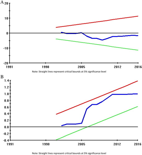
Figure 1 demonstrates plots of CUSUM and CUSUMSQ for Models 1–3. The CUSUM and CUSUMSQ plots show that the ARDL parameters in all the models are stable at 5% bounds. The stability of parameters over time is reflected through the graphical plots of CUSUM and CUSUM sum of squares (Figures 1(A,B), 2(A,B) and 3(A,B), respectively).

Figure 1. (A) Plot of cumulative sum of recursive residuals (Model 1). (B) Plot of cumulative sum of squares of recursive residuals (Model 1).

Note: Straight lines represent critical bounds at 5% significance level.

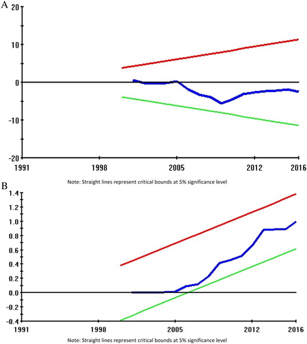
Figure 2. (A) Plot of cumulative sum of recursive residuals (Model 2). (B) Plot of cumulative sum of squares of recursive residuals (Model 2).

Note: Straight lines represent critical bounds at 5% significance level.

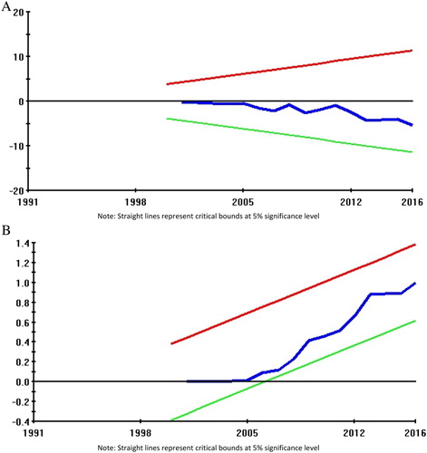
Figure 3. (A) Plot of cumulative sum of recursive residuals (Model 3). (B) Plot of cumulative sum of squares of recursive residuals (Model 3).

Note: Straight lines represent critical bounds at 5% significance level.

Toda Yamamoto causality results are reported in Table 9. Causal findings reveal that there exists bidirectional causality between globalisation and the indicators of poverty and between corruption and some indicators of poverty. Statistical significance is evident when the null hypotheses of no causality are rejected based on p-values.

Table 9. Toda Yamamoto causality test results.

	χ^2	Prob.		χ^2	Prob.
ΔlnMR → ΔlnLE	2.182878	0.1396	ΔlnLE → ΔlnMR	7.291313	0.0069
ΔlnHC → ΔlnLE	2.090599	0.1482	ΔlnLE → ΔlnHC	0.045276	0.8315
ΔGLO → ΔlnLE	0.785379	0.3755	ΔlnLE → ΔGLO	0.001880	0.9654
ΔCOR → ΔlnLE	1.835296	0.1755	ΔlnLE → ΔCOR	0.001911	0.9651
ΔlnHC → ΔlnMR	0.004476	0.9467	ΔlnMR → ΔlnHC	5.288921	0.0215
ΔGLO → ΔlnMR	0.893577	0.3445	ΔlnMR → ΔGLO	0.013947	0.9060
ΔCOR → ΔlnMR	0.165253	0.6844	ΔlnMR → ΔCOR	0.147764	0.7007
ΔGLO → ΔlnHC	0.457662	0.4987	ΔlnHC → ΔGLO	0.293853	0.5878
ΔCOR → ΔlnHC	0.080197	0.7770	ΔlnHC → ΔCOR	0.131983	0.7164
ΔCOR → ΔGLO	1.398093	0.2370	ΔGLO → ΔCOR	3.367715	0.0665

Results from the variance decomposition analysis are reported in Tables 10–12. Findings from all models suggest that globalisation and corruption will potentially have some negative effect on poverty in future across all three poverty indicators measured.

Table 10. Variance decomposition results (lnHC).

Period	LNHC	GLO	COR	LNGDPPC	INQ	LNFD	LNFDI	LNEDU	INT	LNMOB
1	100.000000	0.000000	0.000000	0.000000	0.000000	0.000000	0.000000	0.000000	0.000000	0.000000
2	68.311740	0.865366	0.129216	16.481910	6.797510	0.385963	0.942674	5.729493	0.191517	0.164616
3	57.776530	1.497676	0.515634	22.704340	7.939065	1.847063	1.342232	6.107837	0.141504	0.128117
4	52.915920	1.324243	0.829904	23.766960	10.756640	2.263296	1.874244	6.014178	0.125626	0.128988
5	51.257100	1.325965	0.818373	23.908630	11.865400	2.278943	1.898015	6.378190	0.145415	0.123964
6	50.484870	1.315468	0.823451	24.056890	12.113390	2.317670	2.129624	6.465504	0.171888	0.121243
7	49.810800	1.309347	1.034046	24.222450	12.169800	2.345019	2.203275	6.576245	0.210581	0.118444
8	49.084600	1.296670	1.247237	24.560700	11.998560	2.408416	2.375505	6.655259	0.257842	0.115204
9	48.380950	1.281815	1.543470	24.839800	11.841000	2.490328	2.504687	6.686404	0.318864	0.112678
10	47.658310	1.259739	1.892165	25.094600	11.653690	2.561030	2.658575	6.722557	0.389013	0.110319

Table 11. Variance decomposition results (lnMR).

Period	LNMR	GLO	COR	INT	INQ	LNEDU	LNFD	LNFDI	LNGDPPC
1	100.0000	0.000000	0.000000	0.000000	0.000000	0.000000	0.000000	0.000000	0.000000
2	80.16816	7.394742	2.086054	2.010177	1.527093	1.347602	0.354489	3.438348	1.673338
3	75.91277	8.964175	1.960760	2.157399	1.792160	1.568959	0.531718	5.252509	1.859548
4	72.64801	8.919575	2.507663	2.083936	1.795996	1.787107	0.518928	7.956260	1.782526
5	70.87407	8.757911	2.820424	2.235006	2.291796	2.146066	0.507319	8.594587	1.772823
6	70.49834	8.806950	2.876062	2.438634	2.279848	2.230738	0.504572	8.595204	1.769656
7	70.27884	8.933321	2.951561	2.451202	2.281177	2.263675	0.508038	8.568768	1.763418
8	70.15475	8.946582	2.984773	2.537653	2.276958	2.260622	0.507088	8.567714	1.763860
9	70.04677	8.975508	3.011976	2.590023	2.276732	2.261678	0.506318	8.569423	1.761569
10	69.95610	8.995550	3.029070	2.657409	2.274074	2.259315	0.506888	8.561950	1.759641

Table 12. Variance decomposition results (lnLE).

Period	LNLE	GLO	COR	INQ	INT	LNEDU	LNFD	LNFDI	LNGDPPC
1	100.0000	0.000000	0.000000	0.000000	0.000000	0.000000	0.000000	0.000000	0.000000
2	94.69130	0.672902	1.769843	0.463700	1.265251	0.170520	0.853577	0.106752	0.006154
3	88.65463	2.350125	2.986296	1.251996	3.008527	0.120486	1.363680	0.254861	0.009395
4	83.58421	4.008996	2.955973	1.741085	5.268558	0.082939	1.476110	0.838814	0.043311
5	79.58829	5.267447	2.636935	1.775353	7.763397	0.060039	1.417532	1.406359	0.084646
6	76.29787	6.032203	2.290769	1.600051	10.37354	0.045368	1.352092	1.889179	0.118924
7	73.49844	6.443330	1.981017	1.363900	12.95793	0.036126	1.344928	2.233862	0.140463
8	71.01530	6.625647	1.720879	1.145151	15.45687	0.029808	1.407205	2.448620	0.150520
9	68.72246	6.666488	1.501030	0.968076	17.85837	0.025215	1.535732	2.569451	0.153180
10	66.53381	6.622501	1.312924	0.835130	20.17408	0.021754	1.716475	2.631734	0.151592

5. Discussion

This article investigated the dynamic effects of globalisation and corruption on poverty in South Africa between 1991 and 2016, allowing for a set of control variables including economic growth, ICT diffusion and adherence to the rule of law. South Africa’s increasing integration into the global economy, combined with clear signs of increasing corruption provide sufficient reason to examine the effect of both indicators on poverty. There are only a few extant studies that have investigated these, especially in a country specific, time series context.

In this study, as part of the econometric procedures for estimating the empirical association between the variables, the Zivot–Andrews structural break unit root test was conducted to assess the stationarity of data in the presence of structural breaks. As variables were found to have a mixed order of integration, ARDL bounds testing was employed to estimate the short-run and long-run effects of globalisation and corruption on the three selected indicators of poverty. The Toda Yamamoto causality test was conducted to examine the causal link between poverty, globalisation and corruption. To assess whether or not the findings are robust, variance decomposition analysis was then performed.

The findings reveal that globalisation reduces poverty in the long run across all three specifications of the dependent variable. In the short run, globalisation reduces both the poverty headcount and the infant mortality rate. Corruption, however, leads to an increase in poverty in all model specifications, mainly on the poverty headcount in the short run. Causality findings confirm bidirectional causality of both globalisation and corruption with the indicators of poverty but without significance in many cases. In summary, these quantitative estimates generally support the a priori expected results of a positive effect of globalisation and a negative effect of corruption, on poverty in South Africa.

The most common approach to measuring poverty is the headcount or absolute poverty measure. However, this method has been widely criticised in the literature for its simplistic nature. Therefore, in this study three different indicators of poverty have been included as the dependent variable; a direct measure – headcount or absolute poverty and two indirect measures – infant mortality rate and life expectancy. Those three indicators are used independently for estimation purposes and to cross-check the estimates obtained. The results of the three measures indicate the limited value of the headcount indicator.

The core independent variables are globalisation and corruption. Most studies in the literature use trade integration (trade as a share of GDP) as a rather simplistic measure of globalisation. The KOF index which measures globalisation across economic, social and political dimensions was used and produced robust inputs as it allows for a separate analysis of economic flows and trade policies. Corruption is also a multidimensional concept and a very popular measure widely used is the Corruption Perceptions Index of Transparency International but it has poor data reliability from year to year, since corruption is, by its nature, difficult to observe. The World Bank World Governance Indicators comprises six indicators, including control of corruption and the rule of law and have good year to year data reliability.

5.1. Policy implications

The study has a number of policy implications. First, South Africa is enjoying some pay-offs from its long and persistent trade liberalisation efforts, with the expansion of formal employment seemingly the main factor contributing to the observed reduction in poverty from globalisation. Trade liberalisation has resulted in the expansion of the formal sector over recent years in South Africa, particularly for low-skilled and skilled workers (Bureau of Economic Research, 2018). These gains could be reversed by appeals for domestic economic protection via tariffs and other non-trade barriers.

The study results also lend credence to the hypothesis that corruption intensifies poverty. It may be argued that corruption and challenges to the rule of law (domestic security) might be key stumbling blocks towards the effectiveness of the many poverty reduction initiatives undertaken. Many prospective and highly potential foreign nationals have been engaged in different types of businesses in South Africa for decades, contributing to local employment and the economy, but this flow of foreign investment has slowed recently mostly due to deteriorating law and order. Good governance and the elimination of corruption is a must for improving the performance of all sectors of an economy. To achieve good governance, key state institutions, must be protected and strengthened. Otherwise, a lack of good governance will further exacerbate corruption which will further impoverish the nation.

5.2. Study limitations

This study suffers from a number of caveats. First, poverty, globalisation and corruption are all multidimensional and multifaceted concepts, with different sources constructing the measures in different ways. No consensus has yet been reached on their unique and undisputed measurement. Past empirical studies provide widely varied outcomes due to the heterogeneity in such measurements. Second, the findings should be generalised with caution, as different studies use different methodologies, datasets, sample periods and coverage of countries and regions.

Disclosure statement

No potential conflict of interest was reported by the authors.

References

- Adebayo, AA, 2013. The nexus of corruption and poverty in the quest for sustainable development in Nigeria. Journal of Sustainable Development in Africa 15, 225–35.
- Agénor, P-R, 2004. Does globalization hurt the poor? International Economics and Economic Policy 1(1), 21–51. doi: 10.1007/s10368-003-0004-3
- Attanasio, O, Goldberg, P & Pavenik, N, 2004. Trade reforms and wage inequality in Colombia. Journal of Development Economics 74, 331–66. doi: 10.1016/j.jdeveco.2003.07.001
- Basu, K, 2006. Globalization, poverty, and inequality: What is the relationship? What can be done? World Development 34(8), 1361–73. doi: 10.1016/j.worlddev.2005.10.009
- Ben Ali, MS, Cockx, L & Francken, N, 2016. The Middle East and North Africa: Cursed by natural resources? In Ben Ali, M-S (Ed.), Economic development in the Middle East and North Africa, challenges and prospects. Palgrave Macmillan, New York.
- Ben Ali, MS & Sassi, S, 2016. The corruption-inflation nexus: Evidence from developed and developing countries. The BE Journal of Macroeconomics 16(1), 125–44.
- Bergh, A & Nilsson, T, 2014. Is globalization reducing absolute poverty? World Development 62, 42–61. doi: 10.1016/j.worlddev.2014.04.007
- Bologna, J & Ross, A, 2015. Corruption and entrepreneurship: evidence from Brazilian municipalities. Public Choice 165, 59–77. doi: 10.1007/s11127-015-0292-5
- Bureau of Economic Research, 2018. Ten years after the Lehman collapse: South Africa’s post-crisis performance in perspective. Research note 1, 2018. Bureau of Economic Research, Stellenbosch.
- Cieślik, A & Goczek, L, 2018. Control of corruption, international investment, and economic growth – Evidence from panel data. World Development 103, 323–35. doi: 10.1016/j.worlddev.2017.10.028
- Desai, RM & Rudra, N, 2018. Trade, poverty, and social protection in developing countries. European Journal of Political Economy. doi:10.1016/j.ejpoleco.2018.08.008.
- Dincer, C & Gunalp, B, 2008. Corruption, income inequality and poverty in the United States. Working paper 54. Fondazione Eni Enrico Mattei, Milan.
- Dollar, D & Kraay, A, 2004. Trade, growth and poverty. The Economic Journal 114(493), F22–F49. doi: 10.1111/j.0013-0133.2004.00186.x
- Dowrick, S & DeLong, JB, 2001. Globalisation and convergence. Paper presented at the NBER Conference in Historical Perspective, 4–5 May, National Bureau of Economic Research, Cambridge, MA, USA.
- Dreher, A, 2006. Does globalization affect growth? Evidence from a new index of globalization. Applied Economics 38(10), 1091–110. doi: 10.1080/00036840500392078
- Dreher, A & Gassebner, M, 2013. Greasing the wheels? The impact of regulations and corruption on firm entry. Public Choice 155(3-4), 413–32. doi: 10.1007/s11127-011-9871-2
- Duasa, J, 2007. Determinants of Malaysian trade balance: An ARDL bound testing approach. Global Economic Review 36(1), 89–102. doi: 10.1080/12265080701217405
- Engle, RF & Granger, CWJ, 1987. Co-integration and error correction: Representation, estimation, and testing. Econometrica 55, 251–76. doi: 10.2307/1913236
- Erten, B, Leight, J & Tregenna, F, 2019. Trade liberalization and local labor market adjustment in South Africa. Journal of International Economics 118, 448–67. doi: 10.1016/j.jinteco.2019.02.006
- Fransman, T & Yu, D, 2018. Multidimensional poverty in South Africa in 2001–16. Development Southern Africa 36(1), 50–79. doi: 10.1080/0376835X.2018.1469971
- Ghobarah, HA, Huth, P & Russett, B, 2004. The post-war public health effects of civil conflict. Social Science & Medicine 59, 869–84. doi: 10.1016/j.socscimed.2003.11.043
- Goldberg, P & Pavcnik, N, 2003. The response of the informal sector to trade liberalization. Journal of Development Economics 72, 463–96. doi: 10.1016/S0304-3878(03)00116-0
- Gossel, SJ, 2018. FDI, democracy and corruption in Sub-Saharan Africa. Journal of Policy Modeling 40, 647–62. doi: 10.1016/j.jpolmod.2018.04.001
- Granger, CWJ, 1969. Investigating causal relations by econometric models and cross-spectral methods. Econometrica 37, 424–38. doi: 10.2307/1912791
- Gupta, S, Davoodi, H & Alonso-Terme, R, 2002. Does corruption affect income inequality and poverty? Economics of Governance 3(1), 23–45. doi: 10.1007/s101010100039
- Ha, E & Cain, NL, 2017. Who governs or how they govern: Testing the impact of democracy, ideology and globalization on the well being of the poor. The Social Science Journal 54, 271–86. doi: 10.1016/j.soscij.2017.01.010
- Harris, R & Sollis, R, 2003. Applied time series modeling and forecasting. Wiley, West Sussex.
- Hérault, N, 2006. Building and linking a microsimulation model to a CGE model for South Africa. South African Journal of Economics 74, 34–58. doi: 10.1111/j.1813-6982.2006.00047.x
- Hessami, Z, 2014. Political corruption, public procurement, and budget composition: theory and evidence from OECD countries. European Journal of Political Economy 34, 372–89. doi: 10.1016/j.ejpoleco.2014.02.005
- Hoffman, P, 2012. The effect of corruption on poverty. Accountability Now, Johannesburg. https://accountabilitynow.org.za/effect-corruption-poverty/ Accessed 10 January 2019.
- Huntington, S, 1968. Political order in changing societies. Yale University Press, New Haven.
- Husted, BW, 1999. Wealth, culture and corruption. Journal of International Business Studies 30(2), 339–59. doi: 10.1057/palgrave.jibs.8490073
- Ibrahim, MH, 2005. Sectoral effects of monetary policy: Evidence from Malaysia. Asian Economic Journal 19, 83–102. doi: 10.1111/j.1467-8381.2005.00205.x
- Justesen, MK & Bjørnskov, C, 2014. Exploiting the poor: Bureaucratic corruption and poverty in Africa. World Development 58, 106–15. doi: 10.1016/j.worlddev.2014.01.002
- Kaplinsky, R, 2002. Spreading the gains from globalisation: What can be learned from value chain analysis. IDS working paper 110. Institute of Development Studies, University of Sussex, Sussex.
- Kis-Katos, K & Sparrow, R, 2015. Poverty, labor markets and trade liberalization in Indonesia. Journal of Development Economics 117, 94–106. doi: 10.1016/j.jdeveco.2015.07.005
- Kitson, M & Michie, J, 1995. Trade and growth: A historical perspective. In Michie, J & Smith, JG (Eds.), Managing the global economy. Oxford University Press, Oxford.
- Klitgaard, R, 2017. Corruption and development. In Battersby, P & Roy, R (Eds.), International development: A global perspective on theory and practice. Sage, London, 150–64.
- Kozul-Wright, R & Rayment, P, 2004. Globalisation reloaded: An UNCTAD perspective. UNCTAD discussion paper 167. UNCTAD, Geneva.
- Krueger, A, 1983. Trade and employment in developing countries. Synthesis and conclusions. Vol. 3. National Bureau of Economic Research, New York.
- Krueger, A & Berg, A, 2003. Trade, growth, and poverty: A selective survey. IMF working paper, WP/03/30. International Monetary Fund, Washington, DC.
- Le Goff, M & Singh, R, 2014. Does trade reduce poverty? A view from Africa. Journal of African Trade 1, 5–14. doi: 10.1016/j.joat.2014.06.001
- Liyanaarachchi, TS, Naranpanawa, A & Bandara, JS, 2016. Impact of trade liberalisation on labour market and poverty in Sri Lanka. An integrated macro-micro modelling approach. Economic Modelling 59, 102–15. doi: 10.1016/j.econmod.2016.07.008
- Lund, C & Cois, A, 2018. Simultaneous social causation and social drift: Longitudinal analysis of depression and poverty in South Africa. Journal of Affective Disorders 229, 396–402. doi: 10.1016/j.jad.2017.12.050
- Lutkepohl, H, 2006. Structural vector autoregressive analysis for cointegrated variables, AStA. Advances in Statistical Analysis 90, 75–88.
- Magombeyi, MT & Odhiambo, NM, 2018. Dynamic impact of FDI inflows on poverty reduction: Empirical evidence from South Africa. Sustainable Cities and Society 39, 519–26. doi: 10.1016/j.scs.2018.03.020
- Méon, P & Sekkat, K, 2005. Does corruption grease or sand the wheels of growth? Public Choice 122(1/2), 69–97. doi: 10.1007/s11127-005-3988-0
- Negin, V, Rashid, ZA & Nikopour, H, 2010. The causal relationship between corruption and poverty: A panel data analysis. MPRA paper No. 4871. https://mpra.ub.uni-muenchen.de/24871/ Accessed 10 January 2019.
- Nissanke, M & Ferrarini, B, 2001. Debt dynamics and contingency financing: Theoretical reappraisal of the HIPC initiative. UNU-WIDER discussion paper 2001/139. UNU-WIDER, Helsinki.
- Nissanke, M & Thorbecke, E, 2006. Channels and policy debate in the globalization–inequality–poverty nexus. World Development 34(8), 1338–60. doi: 10.1016/j.worlddev.2005.10.008
- Nissanke, M & Thorbecke, E, 2010. Globalization, poverty, and inequality in Latin America: Findings from case studies. World Development 38(6), 797–802. doi: 10.1016/j.worlddev.2010.02.003
- N’zue, FF & N’guessan, CJF, 2006. The causality between corruption, poverty and growth: A panel data analysis. Working paper series. Secretariat for Institutional Support for Economic Research in Africa, Ottawa.
- Olper, A, Curzi, D & Swinnen, J, 2018. Trade liberalization and child mortality: A synthetic control method. World Development 110, 394–410. doi: 10.1016/j.worlddev.2018.05.034
- Pesaran, H & Shin, Y, 1999. An autoregressive distributed lag modeling approach to cointegration. Chapter 11 in Econometrics and economic theory in the 20th century: The Ragnar Frisch Centennial Symposium. Cambridge University Press, Cambridge.
- Pesaran, H, Shin, Y & Smith, R, 2001. Bounds testing approaches to the analysis of level relationships. Journal of Applied Econometrics 16(3), 289–326. doi: 10.1002/jae.616
- Pillay, S, 2004. Corruption – the challenge to good governance: A South African perspective. International Journal of Public Sector Management 17, 586–605. doi: 10.1108/09513550410562266
- Poveda, AC, Carvajal, JEM & Pulido, NR, 2019. Relations between economic development, violence and corruption: A nonparametric approach with DEA and data panel. Heliyon. doi:10.1016/j.heliyon.2019.e01496.
- Rahayu, IP & Widodo, T, 2012. The causal relationship between corruption and poverty in ASEAN: A general method of moments/ dynamic panel data analysis. Journal of Economics, Business, and Accountancy | Ventura 15(3), 527–36. doi: 10.14414/jebav.v15i3.119
- Ravallion, M, 2003. The debate on globalization, poverty and inequality: Why measurement matters. International Affairs 79, 739–53. doi: 10.1111/1468-2346.00334
- Salvatore, D, 2004. Growth and poverty in a globalizing world. Journal of Policy Modeling 26, 543–51. doi: 10.1016/j.jpolmod.2004.04.009
- Singh, R & Huang, Y, 2011. Financial deepening, property rights and poverty: Evidence from Sub-Saharan Africa. IMF working paper, WP/11/196, Washington. International Monetary Fund, Washington, USA.
- Statistics South Africa, 2018. Poverty on the rise in South Africa. http://www.statssa.gov.za/?p=10334 Accessed 18 June 2019.
- Swiss Economic Institute, 2018. KOF Globalisation Index. https://www.kof.ethz.ch/en/forecasts-and-indicators/indicators/kof-globalisation-index.html Accessed 10 January 2019.
- Tanzi, V, 1995. Corruption, arm’s-length relationships, and markets. In Fiorentini, G & Peltzman, S (Eds.), The economics of organised crime. Cambridge University Press, Cambridge, MA.
- Thurlow, J, 2006. Has trade liberalization in South Africa affected men and women differently? DSGD discussion paper no. 36. IFPRI, Washington, DC.
- Toda, HY & Yamamoto, T, 1995. Statistical inference in vector autoregressions with possibly integrated processes. Journal of Econometrics 66, 225–50. doi: 10.1016/0304-4076(94)01616-8
- Transparency International, 2019. Corruption Perceptions Index. https://www.transparency.org/cpi2018 Accessed 10 January 2019.
- Tsai, P & Huang, C, 2007. Openness, growth and poverty: The case of Taiwan. World Development 35, 1858–71. doi: 10.1016/j.worlddev.2006.11.013
- Ugur, M, 2014. Corruption’s direct effects on per-capita income growth: A meta-analysis. Journal of Economic Surveys 28(3), 472–90. doi: 10.1111/joes.12035
- World Bank, 2015. Sri Lanka ending poverty and promoting shared prosperity. World Bank, Washington, DC.
- World Bank, 2017. World development indicators database. http://data.worldbank.org/indicator/all Accessed 10 January 2019.
- World Bank, 2018. Worldwide governance indicators. http://info.worldbank.org/governance/wgi/index.aspx#doc Accessed 17 June 2019.
- Zivot, E & Andrews, D, 1992. Further evidence of on the great crash, the oil price shock and the unit root hypothesis. Journal of Business and Economic Statistics 10, 251–70.