Heterogeneous relationships between income levels and associated correlates in Gauteng province, South Africa: quantile regression approach

ABSTRACT

Despite implementation of several government policies since the dawn of democracy in South Africa, income distribution remains skewed in the country. This paper explores income distribution in the Gauteng province by addressing two important questions: first, what is the level and pattern of income distribution, and second, do the role of correlates in explaining income distribution differ across income groups? By employing quantile regression analysis, this paper’s results not only show the explanatory role of various correlates, such as race, but it also confirm that the explanatory role of these correlates is heterogeneous across income groups. The paper by drilling down into the data established that there are variations across some identifiable groups (e.g. youth, pensioners, and adults) and quantiles. These results enable policy makers to tailor policies to specific income and other identifiable groups, rather than one-size-fit-all policy focus.

KEYWORDS:

• Income levels
• heterogeneous relationship
• quantile regression
• Gauteng province
• South Africa

JEL CLASSIFICATIONS:

• D14
• D31
• H24
• R11

1. Introduction

South Africa, like many other sub-Saharan African (SSA) and developing countries, has pervasive development inequalities. Comparable data from the UNU-WIDER (2017) show the least Gini coefficient of 30.82 (Sao Tome), a highest Gini coefficient of 74.3 (Namibia), and a median Gini coefficient of 39.35. South Africa’s Gini coefficient has been declining, but at a very slow pace. For instance, post 2008–09 financial crisis, South Africa’s income-based Gini coefficient of 70 in 2009 declined marginally to 67.52 by 2014, then increased to reach 68.65 in 2018. Without social grants, South Africa’s income-based Gini coefficient of 74.44 in 2009 declined to 71.99 in 2014, then increased to reach 73.59 in 2018 (EasyData, 2019).

With income inequalities prominent along racial groups, and urban and rural areas, reducing income inequality in the country remains a serious developmental challenge. Past empirical work from many studies focusing on income inequality and poverty provide consensus that the former poses far more challenges to economic growth and poverty reductions, etc. (see, for example, Ravallion, 2001 and Tregenna, 2011). These worrying results happen in the backbone of a government that has gone all throttle to address income inequalities and poverty since 1994 through various policies. Shifting ideological debates and policy imperatives over the years partly have curtailed the success of these policies.¹ In Gauteng province, little success have been achieved in addressing income inequality. Moreover, with Gauteng province being the largest agglomeration – contributing about a third of national GDP, thus exerting a significant influence over the lives of the people of South Africa (OECD, 2011) – this paper’s focus on income distribution and inequality in the province is timely.

EasyData (2019) data shows that Gauteng’s income-based Gini coefficient of 66 in 2009 declined marginally to 62.78 by 2014, then rose to 65.13 in 2018. Without social grants, Gauteng’s income-based Gini coefficient of 67.54 in 2009 declined to 64.63 in 2014, then rose to 67.57 in 2018. With most measures, including income and non-income measures showing persisting inequalities across race groups and localities in Gauteng province, there is need for further research. This paper contributes to the existing literature on income distribution and inequality in Gauteng province and beyond. It addresses two important and pending questions. First, what is the level and pattern of income distribution and inequality in Gauteng province, and second, do the role of correlates in explain the level and pattern of income inequality differ across income groups?

The remainder of the paper is structured as follows. After the introduction, Section 2 reviews related literature, including a reflection on empirical work related to quantile regression analysis. Section 3 describes data and methods, including the study area, description of variables, as well as choice of analytical techniques. Section 4 dwells on results and related discussions, while the last section concludes the paper.

2. Review of related literature

2.1. Income inequality research

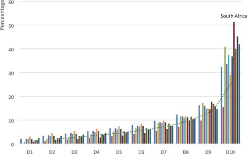
Inequality in SSA is perverse. Data from UNU-WIDER (2017) for several SSA countries show the least Gini coefficient of 30.82 (for Sao Tome), a highest Gini coefficient of 74.3 (for Namibia), and a median of 39.35. Although the data are for different years, there is no evidence to suggest that even with updated data; there would be a significant reduction in inequality among these countries. In Southern African region, South Africa shows more inequality compared to its neighbours. For example, Figure 1 shows the share of decile in income distribution for South Africa and its neighbours. The general trend is that of increasing share of income from the lowest to the highest deciles for all countries. The figure shows the prominent share of the highest deciles in South Africa. The smoothed trend line based on a 2-span weighted moving average shows the share of income progressively increasing and strengthening from lower to higher deciles.

Figure 1. Income distribution in Southern Africa: Share of deciles in income distribution. Source: UNU-WIDER (2017) for various years in each country – Angola (2008), Botswana (2009), Lesotho (2010), Madagascar (2012), Malawi (2010), Mauritius (2012), Mozambique (2008), Namibia (2010), South Africa (2011), Swaziland (2009), and Zambia (2010).

There is a rich list of existing literature on income inequality in developing countries, including South Africa. A few are reviewed here. Elbers et al. (2008) in their multi-country (including South Africa) study found that race, education levels, and the location (either rural or urban) of the household had an impact on households income. In his multi-country research, Glaeser (2005) notes that inequality levels differ wildly. He notes that inequality is correlated with a number of important variables, including ethnic heterogeneity, skill levels, and political economy variables (e.g. dictatorship, property rights). He cautions, however, that the nature of correlation is not straightforward at all times. For instance, he explains that if education and skill levels in input are non-homogeneous, inequality in output is likely to be high as well.

Okojie & Shimiles (2006) reviewed research on income and non-income inequalities focusing on SSA. Their results showed evidence of income differences between urban and rural areas and between gender, levels of education, and levels of infrastructure development. They also showed that demographic variables (e.g. large ethnic diversity and population density) have explanatory power on income differences.

In South Africa, Deaton (1997) showed that blacks were not only poorer than whites, but their living standards were more unequally distributed. He further showed that blacks were worse off than coloureds, Indian and whites. Deaton’s inequality measures are not surprising since inequality was entrenched in the policies of the apartheid government and in the history of the country generally (see Table 3.4 in Deaton, 1997:157).

Elsewhere, new data from StatsSA² has heralded income and poverty studies in South Africa. Often, across various measures of inequality, the blacks are worse off, followed by coloureds, Indians/Asians, and whites (Bhorat et al., 2009:53; Leibbrandt et al., 2009). There is also evidence of income variation within race groups (Bhorat et al., 2009). Existing literature also show that beyond race explaining income inequality, education (and particularly skill levels), location (either urban or rural or township or suburbs), and demographic variables (e.g. gender, migration status) also explain income inequality.

2.2. Quantile regression analysis approach

Since the pioneering work of Koenker and Bassett (e.g. Bassett & Koenker, 1978; Koenker & Bassett, 1978) there has been growth in empirical literature employing models that go beyond the conditional mean, typical of the least squares estimating procedures, to incorporate estimation based on conditional quantile functions. The latter are models in which quantiles of the conditional distribution of the response variable are expressed as functions of observed covariates (Koenker & Bassett, 2001:147). These empirical literature (covering developed and developing world) have addressed issues in the labour markets, school quality, demand analysis, finance, earning inequality and mobility, etc. (see Koenker & Hallock, 2001:151–2 for a selected review of these empirical work).

Schultz & Mwabu (1998) used a sample of 6016 employed (16–64 years) respondents collected by the SALDRU at the University of Cape Town in late 1993 (SALDRU, 1994). Their analysis showed that among male African workers in the bottom decile of the wage distribution, union membership was associated with wages that were 145% higher than those of comparable non-union workers, and among those in the top decile the differential was 19%. Moreover, Schultz & Mwabu (1998) found that returns to observed productive characteristics of workers, such as education and experience, were larger for non-union than union workers. Their results further suggested that if the large union relative wage effect were cut in half, the estimate showed that employment of African youth, age 16–29 years, would increase by two percentage points, and their labour force participation rate would also increase substantially.

In another study focusing on education returns across quantiles of the wage function, Mwabu & Schultz (1996) compared ordinary least square (OLS) and quantile regressions estimates and found interesting results with regard to the three levels of schooling for African and white males. They noted that by quantile regression reducing sensitivities to outliers, it informs us how returns vary across quantiles. For instance, they note that returns for Africans decline with increasing decile at higher education and are not linearly related to decile at the secondary level, while among whites the return to higher education increases significantly with decile, from 9% at the bottom (0.1 decile) to 18% at the top (0.9 decile) (Mwabu & Schultz, 1996:338).

Kwenda & Ntuli (2018) undertook a detailed decomposition of public-private sector wage gap in South Africa for 2000–14. Using unconditional quantile regressions as one of the techniques, they found that gender, age, marital status, education, occupation, and race have a role in explaining income inequality. Similarly, Finn & Leibbrandt (2018) identified education and the length of experience as drivers of changes in the distribution of earnings and earnings inequality in the South African labour market between 2000 and 2014. This paper adds to the existing rapporteur of studies on income distribution and inequality by employing quantile regression approach – a technique missing in the existing South African literature focusing on household or per capita income.

3. Data and methods

3.1. Study area

This study focuses on Gauteng province that is at the core of the Gauteng city-region. The city-region measures about 2% of national land mass and represents an integrated cluster of cities, towns and urban nodes to make the country’s largest economic agglomeration (see Figure 2 showing its location). The GCR’s economic footprint extends to the neighbouring provinces of Free State, Mpumalanga and North West. It thus shapes the growth or otherwise of the national economy and in the process exert a significant influence over the lives of the people of South Africa (OECD, 2011).

Figure 2. Gauteng province and its surroundings – forming the wider Gauteng city-region.

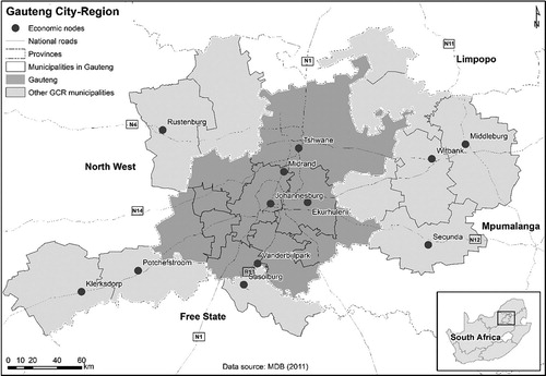
However, the Gauteng province (and by extension the GCR) has inherent placed-based economic features that bring both prosperity and despair. Existing literature (e.g. Presidency, 2006:72–3; Cheruiyot, 2018) show that Gauteng province has, not only, high levels of economic potential (as indicated by high GVA and relatively diverse economic activities, etc.), but also high levels of poverty (large numbers of people living below the Minimum Living Level) and huge disparities in income and access to services, etc.

Available data from EasyData (2019) show that in 2017 Gauteng province alone contributed 34.19% of national GVA, while the wider GCR accounted for 43.2% of the national GVA. Gauteng province accommodates about 14.7 million people, contributing a quarter of the national population. Gauteng province, thus, has the highest population density than the other eight provinces in the country (EasyData, 2019).

Gauteng province has a slightly lower expanded unemployment (34.4%) than the expanded national unemployment rate (37.2%) (StatsSA, 2018).³ There are consequently significant poverty effects in the province, for instance, in 2010 headcount rate (in %) was 29.2 and 18.9, based on StatsSA’s upper (= R577 a month poverty line) and lower (= R416 a month poverty line) bound, respectively (Mushongera et al., 2018). In both measures, Africans are worse off, followed by coloureds, Indian/Asian, and Whites. The continued juxtapositioning of opportunity and marginalisation needs a dedicated research that would inform appropriate policies.

3.2. Data

This paper uses the 2015 Gauteng City-Region Observatory’s (GCRO, 2015a) QoL survey (QoL IV) data obtained by interviewing adults (18 years and over) in Gauteng province. To achieve ward representivity, a minimum number of 30 and 60 interviews were conducted in non-metropolitan and metropolitan municipalities, respectively. Other steps undertaken to ensure representivity, include employing random sampling where replacement interviews were conducted from the Small Area Layer (SAL)⁴ as well as weighting according to population proportional to size (PPS). The SAL-based interviews were eventually aggregated to ward level, municipal level, and lastly, provincial level, where a sample of 30 002 respondents was realised. Ultimately, the results were weighted back to Census 2011 (StatsSA, 2011) in terms of the key demographic variables of gender, race, and geography (for a complete explanation of sampling methodology and weighting, see GCRO (2015b:4)).

The dependent variable in the paper is per capita monthly income – categorisation of income bands mirrors StatsSA’s categorisation. With the individual (geocoded at interview location) as the unit of analysis, several explanatory variables were hypothesised as (correlates) of monthly per capita income. The choice of explanatory variables was informed, largely, by the existing data as well as empirical work (e.g. Finn & Leibbrandt, 2018; Kwenda & Ntuli, 2018; see review literature above). The analysis is based on respondents who were in some form of employment (n = 14 847). Restricting the analysis to individuals with at least R1, a final sample size of 8567 was realised. The use of 8567 individuals was easily achieved by invoking the ‘na.action = na.omit’ in R studio modelling.

Table 1 contains the description of the dependent and explanatory variables used in the paper. The use of categorical or nominal variables, where applicable, was informed by data availability (how the data was recorded) as well as the attempt to drill down into the data to facilitate needed policy suggestions. For instance, while the age variable was recorded as a continuous variable, it serves little to know that age is positively related to income, that is, as respondents’ age rises so is their levels of income and vice versa. Rather, it is more important for policy formulation to know which group, say youth or pensioners, earns less or more, than adult population and at which quantile. The same logic applies to the other categorical or nominal variables.

Table 1. Description of model variables.

Variable	Measurement scale	Description
Income	Continuous	Per capita income
Race	Nominal	0 for Africans/blacks. 1 if coloured. 2 if Indian/Asians. 3 if white
Gender	Nominal	0 for household head is female. 1 if household head male
Age cohort	Nominal	0 for Adult (35–64 years). 1 if youth (18–34 years). 2 if Pensioners (65+ years)
Marital or relationship status	Nominal	0 for those in a relationship. 1 for those not married or in relationship
Education level	Continuous	Total number of years of school/college attendance
Business ownership	Nominal	0 for not owning business. 1 for those who owns a business
Household location	Nominal	0 for Ekurhuleni and the rest of the 8 metros taking a value from 1 to 8, accordingly.
Migration status	Nominal	0 for born in Gauteng. 1 for born in another province in South Africa. 2 born outside South Africa
Disability	Nominal	0 if household head has some disability. 1 for no disability
Sector	Nominal	0 if working in primary sector. 1 if working in secondary or tertiary sector

3.3. Choice of analytical techniques

This study employed quantile regression analysis. The choice of the technique was informed by the nature of the data. With the conditional mean of quantiles represented by x, and the conditional median represented by a dot, it is evident in Figure 3 that to adopt least squares estimation, where the conditional mean and median are varying is inappropriate, as this will lead to non-robust results. Accordingly, segmenting the sample into subsets defined according to the conditioning covariates was a valid option. The use of binary response models (e.g. logit or probit models) with arbitrary probability cut-offs levels, while it could have improved the results, quantile regression analysis was still more natural as suggested by Koenker & Hallock (2001:147).

Figure 3. Income distribution by quantiles in QoL IV survey data.

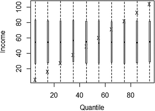
In addition, as a non-parametric technique, the use of quantile regression is appropriate when dealing with variables, which often are skewed, such as income distribution. Here quantile regression estimation minimises the role of the outliers, if any, in the sample data. Below is the econometric equation that was estimated by invoking rq function in R studio (Koenker, 2015).$\begin{array}{rl}Income& ={\text{β}}_0+{\text{β}}_1\ast Race+{\text{β}}_2\ast Gender+{\text{β}}_3\ast Agecohort+{\text{β}}_4\ast Maritalstatus\\ & +{\text{β}}_5\ast Education+{\text{β}}_6\ast Businessowner+{\text{β}}_7\ast Houselocation\\ & +{\text{β}}_8\ast Migrationstatus+{\text{β}}_9\ast disability+{\text{β}}_{10}\ast Sector+\epsilon \end{array}$where ε is the error term, ${\text{β}}_0$ is the intercept, and ${\text{β}}_0-{\text{β}}_{10}$ are estimated regression coefficients (allowing for two or more dummy coefficients, where applicable) of the various explanatory variables as described in Table 1.

4. Results and discussions

4.1. Descriptive results and related discussions

Table 2 shows the univariate statistics of the model variables. In the table, except for income and education variables, all the other model variables are categorical variables. As can be seen in Table 2, average monthly per capita income range from R29 to R409 600, with a standard deviation of R16 579. The large standard deviation and a small median of R1600 (relative to the mean = R5208) indicate that income distribution in the study area is positively skewed.

Table 2. Univariate statistics of model variables,

Variable	n	Min	Max	Mean	Standard deviation
Per capita income (Rands)	8567	29	409,600	5208	16 579
Race	14 847	0	3	0.73	1.25
Gender	14 847	0	1	0.58	0.49
Age cohort	14 932	0	2	0.46	0.54
Marital or relationship status	14 847	0	1	0.17	0.38
Education level	14 847	0	18	12.31	3.20
Business ownership	14 847	0	1	0.11	0.32
Household location	14 847	0	8	1.50	1.72
Migration status	14 847	0	2	0.46	0.66
Disability status	14 847	0	1	0.97	0.17
Sector	11 129	0	1	0.91	0.28

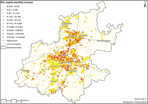
Figure 4 shows average monthly per capita income in Gauteng province (the study area). The data is mapped at the point of interview categorised in quantiles. With income ranging from the lowest of R29 to a high of R409 600 per month, it is evident that the data is not evenly distributed spatially. It shows that the core of the province in areas such as Sandton and Pretoria exhibit high incomes. Pockets of high incomes can also be observed in the areas to the north and south of Johannesburg. Adjacent to these areas, low incomes are visibly distributed. Low incomes are also spread across the province, with Mabopane, Bronkhorstspruit, Vosloosrus, Evaton, Mamelodi, and Soweto as specific examples.

Figure 4. Per capita monthly income in Gauteng.

4.2. Quantile regression results

Table 3 shows the OLS results in the second column and the different quantile regression results in the rest of the columns. Analysis of variance (ANOVA) tests on the nine quantile regressions led to the rejection of the null hypothesis, implying that at least one of the quantile regression is not equal to the others. The pattern of coefficients from lower quantiles to higher quantiles is mixed – for some variables coefficient values increases (e.g. education), some variables’ coefficient values broadly decreases (e.g. sector of employment), while for some variables coefficient values increases and decreases at every turn of the quantile range (e.g. business owner).

Table 3. Quantile regressions results.

Variable	Pooled OLS	tau = 01	02	03	04	05	06	07	08	09
Coloured	–0.079	–30.72	–85.13	–76.46	62.86	–200.11	–302.86	–413.18	–451.85	–1783.39
Indian/Asian	–0.045	–13.63	–6.10	35.10	–52.47	–204.55	–94.29	–91.11	–261.11	–1113.59
White	0.087	31.23	32.83	81.63	155.84	114.29	102.86	79.37	307.41	537.94*
Male	0.242***	46.02***	97.43***	171.70***	294.03***	439.26***	702.86***	1013.02***	1553.70***	2037.86***
Youth	0.051	–11.36	17.43	35.37	49.35	–12.01	14.29	135.71	468.52	1307.57**
Pensioners	0.162	149.35	185.67	286.26	191.17	137.04	28.57	–121.43	231.48	3319.64
Relationship status	0.222***	26.74	95.01**	185.31***	248.83***	360.74***	562.86***	713.33***	1483.33***	2334.89**
Education	0.177***	28.41***	66.05***	108.84***	168.83***	237.62***	320.00***	435.87***	581.48***	898.48***
Business Owner	–0.051	–10.20	4.26	6.12	12.99	–16.88	–120.00	4.76	81.48	–427.26
Johannesburg	0.087	29.33	71.19**	103.13***	151.17**	263.33***	182.86	360.16**	246.30	62.12
Tshwane	0.065	33.83	53.95	67.76**	112.21	204.55**	97.14	280.79	518.52	-224.35
Emfuleni	0.165	83.31	138.89	243.95**	331.95**	279.37	340.00	280.79	970.37	1483.23
Lesedi	0.186	-73.86***	31.61	138.50	62.86	367.14	1217.14**	1153.97	1331.48	2646.87
Midvaal	0.078	39.77	–6.39	125.17	150.65	279.37	145.71	352.38	–83.33	1213.51
Merafong City	0.130	103.19**	95.59	103.13	224.42	330.05	200.00	360.00	570.37	–354.55
Mogale City	–0.033	85.58**	–13.95	–117.55	–74.81	97.78	–182.86	45.71	-70.37	–837.36
West Rand	0.313**	158.68***	276.42***	312.93**	499.22**	496.35***	345.71	518.73	1714.82**	352.94
Born outside Gauteng	0.056	–1.16	19.08	32.38	62.34	81.38	102.86	135.71	272.22	224.35
Foreign born	0.249***	43.70	113.556	216.05***	330.39***	466.40***	1014.29***	1098.57**	2016.67***	3233.36***
Disability	0.187	73.27***	133.03**	170.61	280.00**	418.20***	654.29***	867.94	1187.04**	1134.75
Sector	–0.177***	–73.34**	–57.05	–149.93**	–296.62***	–320.16**	–557.14***	–344.92	–644.44	–2206.05

*** and ** indicate significance at 1%, and 5%, respectively.

Notes: Pooled OLS model was estimated with log-transformed per capita income as the dependent variable. In quantile regressions estimation, per capita income was used, since there was no need to transform the dependent variable (Koenker & Hallock, 2001).

Interpretation of results is as follows. For those variables whose coefficient increase, it implies that the explanatory role of that variable increases as well, as one moves from lower quantiles to higher quantiles. For instance, for the education variable, the coefficient value per quantile changes from a low of R28.41 (for 10% quantile) to a high of R898.48 (for a 90% quantile). This implies that the role of the level of education in explaining income is low for low-income quantile, but increases progressively towards higher-income quantiles in line with human capital theory. Other scholars have found evidence that income differentials can ‘partly be explained the ever-increasing skill premium paid to highly skilled workers’ (Bhorat & van der Westhuizen, 2008:53). In contrast, variables whose estimates decrease implies that the explanatory role of that variable decreases as one moves from lower quantiles to higher quantiles. The interpretation of dummy coefficients, such as for respondents race group, locality, gender, migration status, marital status, business ownership, gender, and disability status, is with respect to the reference group in each individual case.

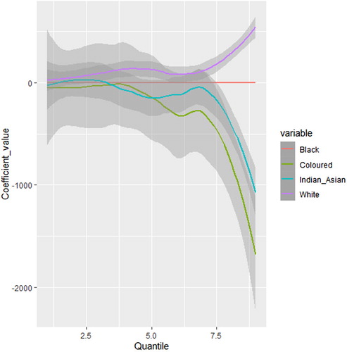
Table 3 shows that among the South African race groups, Africans or blacks was used a reference group. The race variable results in Table 3, although broadly not statistically significant (except in the 90% quantile for whites), show that compared to blacks, coloured, Indian/Asian’s coefficients are smaller, with the difference in incomes more pronounced in the higher quantiles than lower quantiles (see Figure 5). Figure 5 further shows whites’ coefficients were all positive, meaning higher than blacks’ coefficient values of zero. The quantile results specifically show that regression coefficients for white, Indian/Asian, and coloured range from R31.23, –R30.72, and –R13.63 at the lower quantile to R535.94, –R1113.59, and –R1783.39 for the higher quantile, respectively.

Figure 5. Varying coefficients for race variables, with 95% confidence intervals. Blacks was the reference group.

In terms of respondents’ location, Ekurhuleni was used as a reference group. There is a mixture of statistically significant and insignificant results as seen in Table 3. In the OLS model, only the coefficient for West Rand City is statistically significant, implying that respondents in West Rand City earned more than respondents in Ekurhuleni metro. The coefficients for Johannesburg, Merafong City, Lesedi, Emfuleni, Tshwane, and Midvaal are positive, but statistically insignificant in the OLS results. Mogale City’s regression coefficient is negative in the OLS results. In the latter two cases, we can conclude that there was no sufficient evidence that respondents’ incomes in these municipalities were different from respondents’ incomes in Ekurhuleni metro. However, a varied picture is obtained under quantile regression results. On the one hand, the explanatory power of locality in explaining income levels in some municipalities are statistically significant in specific quantiles, while statistically insignificant in other quantiles. For instance, Emfuleni and Mogale City’s coefficients in the 30% (also 40%) and 10% quantiles, respectively, are statistically significant. In these instances, we imply that Emfuleni and Mogale City’s respondents earned more than their counterparts in Ekurhuleni metro (see Figure 7 for the pattern of West Rand City coefficients).

The gender variable had female as the reference group. The statistically significant results show that males earn more than females in the OLS results, as well as in the quantile regressions. In the latter, the amount males earn more than females range from a low of R46.02 for the lower quantile to a high of R2037.86 for the highest quantile. The associated confidence interval width at 95% was uniform from the lower to higher quantiles, implying that males consistently earn more than females regardless of income level (see Figure 6 for graphic presentation of males’ coefficient relative to females’).

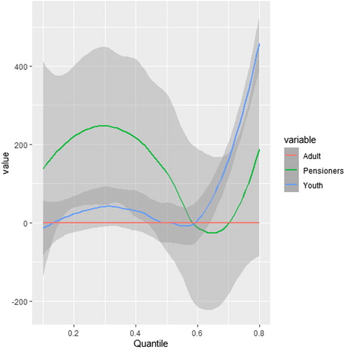
Figure 6. Quantile regression results for pensioners and youth compared to adult (reference group) – with 95% confidence intervals.

The migration variable had three categories – born in Gauteng, migrated to Gauteng from other South African province, and migrated to Gauteng from outside South Africa (foreigners). With ‘those born in Gauteng’ used as a reference, the results imply that foreign respondents earned more than the respondents born in Gauteng in the OLS results and some of the quantiles, where the results were statistically significant (e.g. in the 30% through to 90% quantile). In the 10% and 20% quantiles, we can infer that there is insufficient evidence to conclude that foreigners in these quantiles earned more than the respondents born in Gauteng. None of the regression coefficients for ‘those who migrated to Gauteng from other South African provinces’ are statistically significant, implying that we cannot conclude that these respondents earned more than respondents born in Gauteng.

Estimation results in Table 3 further indicate that none of the regression coefficients for ‘those who own businesses’ were statistically significant. We there conclude that there is insufficient evidence to conclude that respondents who owned businesses either in the OLS or in the quantile regressions earned differently from those without businesses (the latter group acted as the reference group). Results for the disability variable also show that OLS and some of the quantile regression coefficients (e.g. 30% and 70% quantiles) were statistically insignificant. Only regression coefficients for 10%, 20%, 40%, 50%, 60%, and 80% were statistically significant in quantile regression. In the latter case, we can conclude that respondents who are not disabled in these quantiles earned more than disabled respondents – with the magnitude of differences increasing progressively from lower to higher quantiles.

The results for the age dummy – where three categories were used, that is, youth (18–34 years), adults (35–64 years), and pensioners (65+ years) – are interesting. With adults as a reference group (see red horizontal line in Figure 6), estimation results are broadly statistically insignificant. Only youth’s 90% quantile regression coefficient is statistically significant and positive, implying that youth earned more than adults did in this instance (see Figure 6 for graphical illustration).

Figure 7 further presents, graphically, the varying coefficient values (with 95% confidence intervals) of other selected explanatory variables (see Table 3). The relationship status variable was measured as nominal variable, where ‘those in a relationship’ was used as a reference group. Estimation results in Table 3 indicate that respondents ‘who were not in any relationship’ earned more in pooled OLS results as well as in the quantile regression results (except the 10% quantile). Moreover, earnings of ‘those not in a relationship’ progressively increase from their married or in a relationship counterparts’ earnings from the lower quantiles to higher quantiles (see Figure 7).

Figure 7. Varying estimate values for other selected explanatory variables (with 95% confidence intervals each).

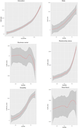
The changing pattern of confidence interval reveals interesting results as well (see Figure 7). For instance, as one moves from lower to higher quantiles for the education plot, the width of the confidence interval decreases, implying that the sample standard deviation decreases. In other words, the results show that variation in income distribution in the higher quantiles is less compared to lower quantiles. A similar broad pattern is observed with regard to the ‘relationship status’ variable. For the male, business ownership, disability, and West Rand City variables, the confidence intervals appear to remain the same – hence little, if any, variations in income distribution in these variables as one moves from lower to higher quantiles.

5. Conclusion

This paper set out to explore income distributions and inequality, measured as per capita income, in Gauteng province using GCRO’s QoL 2015/16 survey data. In doing so, it confirmed that income distribution is skewed – with the respondents in the higher quantiles earning disproportionately more than in the lower quantiles. It further employed quantile regression analysis to explore how different correlates relate to respondents’ income, the latter stratified in quantiles. As suggested by Mosteller & Tukey (1977) and others, the paper drilled down and computed several different regression curves corresponding to the various percentage points of the income distribution – in the process obtaining a more complete picture of the heterogeneous relationship between income and its correlates. In addition, heterogeneous relationships are evident in the varying statistical significance or insignificance across the quantiles for specific variables. This shows evidence or lack of the explanatory role of respective variables, respectively. Often these heterogeneous relationships are masked by other techniques, such as OLS. The paper, thus, contributes to needed debates and methods for addressing income distribution and inequality in Gauteng province and beyond.

The paper further devised the use of categorical or nominal variables, where applicable, rather than the use of continuous variables. It thus successfully drilled down into the data to facilitate needed policy suggestions as well. For instance, while the age variable was recorded as a continuous variable, it serves little to know that income is positively related to income, that is, as respondents’ age rises so are their levels of income and vice versa. Rather, it is more important for policy formulation to know which group, say youth or pensioners, earns less or more, than adult population and at which quantile. This analytical framework was equally useful when applied to other identifiable groups.

Overall, the results not only show the explanatory role of various correlates, such as race, gender, age, marital or relationship status, migration status, business ownership, sector of employment, location, and education, but it also confirms that the explanatory role of these variables is heterogeneous across income groups. These enable policy makers to tailor policies to specific-income and other identifiable groups, rather than one-size-fit-all policy focus, especially that implementation of past policies have led to slow decline in income inequality in the country. Cautiously, we need to take cue from Kwenda & Ntuli (2018) that the manner in which the above factors work to shape income inequality is complex and to succeed we need a broad structural configuration in the economy – a feat not easy to achieve. However, one way would be to undertake policy support scenarios aimed at tackling the structural rigidities that stand in the way of growing the economy and reduction in income inequality, etc. Available models include ADRS’ that can allow policy scenario modelling based on a mix of microeconomic, macroeconomic, trade and industrial, social, private sector, and external policy support strategies (Adelzadeh, 2019).

Disclosure statement

No potential conflict of interest was reported by the author.

Correction Statement

This article has been republished with minor changes. These changes do not impact the academic content of the article.

Notes

1 These policies include Reconstruction and Development Programme (RDP) of 1994–6, Growth, Employment and Redistribution (GEAR) of 1996, the Extended Public Works Programme (EPWP) of 2004, and the Accelerated and Shared Growth Initiative for South Africa (AsgiSA) of 2006. Others are Broad-Based Black Economic Empowerment (BBBEE), New Growth Path (NGP), and National Development Plan (NDP) Vision 2030 (see Cheruiyot & Mushongera, 2018:218–19).

2 These include Quarterly Labour Force Survey (formerly October Household Survey and more recently the Labour Force Survey), the Income and Expenditure Survey, the General Household Survey and the national census.

3 The ‘expanded’ unemployment rate is calculated as the ratio of the number of unemployed, including discouraged work seekers, to the total number of the economically active persons or labour force (which includes the employed, unemployed, and discouraged work seekers). It is considered a true reflection of the development challenge facing governments.

4 Typically made up of two or three Enumerator Areas (EAs), EAs being the lowest StatsSA’s Census statistical geographical unit.

References

- Adelzadeh, A, 2019. Economic policy scenarios for growth and development of South Africa: 2019–2030. Applied Development Research Solutions (ADRS). California, USA & Johannesburg, South Africa.
- Bassett Jr, G & Koenker, R, 1978. Asymptotic theory of least absolute error regression. Journal of the American Statistical Association 73, 618–22. doi: 10.1080/01621459.1978.10480065
- Bhorat, H & van der Westhuizen, C, 2008. Economic growth, poverty and inequality in South Africa: The first decade of democracy. Paper commissioned by The Presidency for the 15 year review process. University of Cape Town (Development Policy Research Unit), Cape Town.
- Bhorat, H, van der Westhuizen, C & Jacobs, T, 2009. Income and non-income inequality in post-apartheid South Africa: What are the drivers and possible policy interventions? Development Policy Research Institute. www.tips.org.za/files/u65/income_and_non-income_inequality_in_post-apartheid_south_africa_-_bhorat_van_der_westhuizen_jacobs.pdf.
- Cheruiyot, K, 2018. City-regions and their changing space economies. In Cheruiyot, Koech (Ed.), The changing space economy of city-regions, 1–24. Springer, Cham.
- Cheruiyot, K & Mushongera, D, 2018. Testing economic growth convergence and its policy implications in the Gauteng city-region. In Cheruiyot, Koech (Ed.), The changing space economy of city-regions, 213–39. Springer, Cham.
- Deaton, A, 1997. The analysis of household surveys: A micro-econometric approach to development policy. World Bank, Washington, DC.
- EasyData, 2019. RSA regional indicators. http://www.quantec.co.za/. Accessed 16 October 2019.
- Elbers, C, Lanjouw, P, Mistiaen, JA & Özler, B, 2008. Reinterpreting between-group inequality. The Journal of Economic Inequality 6, 231–45. doi: 10.1007/s10888-007-9064-x
- Finn, A & Leibbrandt, M, 2018. The evolution and determination of earnings inequality in post-apartheid South Africa. WIDER Working Paper 2018/83. www.wider.unu.edu/sites/default/files/Publications/Working-paper/PDF/wp2018-83_0.pdf.
- GCRO (Gauteng City-Region Observatory), 2015a. Quality of life IV data. Gauteng City-Region Observatory (GCRO), Johannesburg, South Africa.
- GCRO (Gauteng City-Region Observatory), 2015b. Gauteng city-region observatory quality of life 2013 survey: City benchmarking report. Gauteng City-Region Observatory (GCRO), Johannesburg, South Africa.
- Glaeser, EL, 2005. Inequality. NBER Working Paper 2005/11511. National Bureau of Economic Research, Cambridge. www.nber.org/papers/w11511.pdf.
- Koenker, R, 2015. Quantile regression in R: A vignette. www.cran.r-project.org/web/packages/quantreg/vignettes/rq.pdf.
- Koenker, R & Bassett Jr, G, 1978. Regression quantiles. Econometrica: Journal of the Econometric Society 46, 33–50. doi: 10.2307/1913643
- Koenker, R & Hallock, KF, 2001. Quantile regression. Journal of Economic Perspectives 15, 143–56. doi: 10.1257/jep.15.4.143
- Kwenda, P & Ntuli, M, 2018. A detailed decomposition analysis of the public-private sector wage gap in South Africa. Development Southern Africa 35, 815–38. doi: 10.1080/0376835X.2018.1499501
- Leibbrandt, M, Woolard, C & Woolard, I, 2009. Poverty and inequality dynamics in South Africa: Post-apartheid developments in the light of the long-run legacy. In Aron J, Kahn B & Kingdon G (Eds.), South African economic policy under democracy, Chapter 10. Oxford University Press, Oxford, 270–299.
- Mosteller, F & Tukey, JW, 1977. Data analysis and regression: A second course in statistics. Addison-Wesley series in behavioral science: Quantitative methods. Addison-Wesley, Reading, MA.
- Mushongera, D, Tseng, D, Kwenda, P, Benhura, M, Zikhali, P & Ngwenya, P, 2018. Poverty and inequality in the Gauteng city-region. GCRO Research Report No. 09. www.gcro.ac.za/media/reports/GCRO_Research_Report_9_Understanding_poverty_and_inequality_June_2018.pdf.
- Mwabu, G & Schultz, TP, 1996. Education returns across quantiles of the wage function: Alternative explanations for returns to education by race in South Africa. The American Economic Review 86, 335–9.
- OECD, 2011. The Gauteng city-region, South Africa. OECD territorial reviews. OECD Publishing, Paris.
- Okojie, C & Shimeles, A, 2006. Inequality in sub-Saharan Africa. A synthesis of recent research on the levels, trends, effects and determinants of inequality in its different dimensions. Overseas Development Institute, 2–40. www.odi.org/sites/odi.org.uk/files/odi-assets/publications-opinion-files/4058.pdf.
- Presidency, 2006. The national spatial development perspective. The Presidency Policy Coordination and Advisory Services, Pretoria.
- Ravallion, M, 2001. Growth, inequality and poverty: Looking beyond averages. World Development 29, 1803–15. doi: 10.1016/S0305-750X(01)00072-9
- SALDRU (Southern Africa Labour and Development Research Unit), 1994. National income dynamics study. Department of Planning Monitoring and Evaluation, Cape Town & Pretoria.
- Schultz, TP & Mwabu, G, 1998. Labour unions and the distribution of wages and employment in South Africa. ILR Review 51, 680–703. doi: 10.1177/001979399805100407
- StatsSA (Statistics South Africa), 2018. Quarterly labour force survey Q2. Statistics South Africa, Pretoria.
- StatsSA (Statistics South Africa), 2011. Census. Statistics South Africa, Pretoria.
- Tregenna, F, 2011. Halving poverty in South Africa: Growth and distribution aspects. Distribution implications of halving poverty in South Africa. Working Paper No 2011/60. www.semanticscholar.org/paper/Halving-Poverty-in-South-Africa-%3A-Growth-and-of-in-Tregenna/ff61c83f35db75786ec0f2e5a804520d29e814e9.
- UNU-WIDER, 2017. World income inequality database (WIID3.4), January 2017. UNU-WIDER, Helsinki www.wider.unu.edu/database/world-income-inequality-database-wiid34. Accessed 28 October 2018.