Robust Guaranteed-Cost Control for Half-Vehicle Active Suspension Systems Subject to Markovian Controller Uncertainties

Abstract

This paper proposes a robust guaranteed-cost controller for a half-vehicle active suspension system (HVASS) where the controller is subject to stochastic gain fluctuations. This randomly occurring uncertainty is a result of the imperfect implementation of the controller as well as the aging of the components. In this approach, the state-feedback controller is represented via multiple gains orchestrated by a Markovian process, and then an optimal multi-mode design approach with H₂ norm constraints is considered to ensure system’s asymptotic stability with a prescribed disturbance attenuation level. This design is based on Lyapunov theory and the controller is realized via a set of linear matrix inequalities. Compared to the existing works, the design is more reliable for practical HVASSs and is directly reducible to systems with perfectly implemented controllers. Simulation results and comparisons demonstrate the applicability and potentials of the proposed method.

KEYWORDS:

• Markov process
• Uncertainty
• Half vehicle active suspension system
• H₂ Control
• Linear matrix inequality
• Stochastic control

1. INTRODUCTION

Active suspension systems are mechatronic structures that have received increasing attention in recent years [1,2]. They highly affect ride comfort, stability of the vehicle, road handling performance, and suspension deflections. Generally, there exist three suspension systems: passive, semi-active, and active [3]. Passive ones include the conventional springs and dampers; they barely provide satisfactory ride comfort and the road handling capacity. Semi-active suspension systems consisted of springs and variable dampers and lead to considerable improvements over the passive systems but still face limitations in providing ultimate ride comfort and handling. Active suspension systems have actuators parallel to the system assemblies and provide external forces to add or dissipate energy from the system. They perform better in fulfilling the objectives of the suspension control system. Extensive studies have concentrated on the challenges of active suspension control systems considering the conflicting performance criteria [4]. Robust controllers are designed to deal with parametric uncertainties [5,6] and external disturbances [7,8]. Optimal controllers are proposed in [9], fuzzy logic-based structures are given in [10,11], and a wide variety of studies have emphasized on practical limitations such as delay [12,13] and faults [14,15]. Most of the mentioned studies assume that the controllers are going to be implemented perfectly. However, this assumption does not come true in practice and the uncertainty in the controller structure is inevitable. This uncertainty can be caused by factors like faults in the controller components, round-off errors in numerical arithmetic, finite word length in digital systems, and inherent imprecision in the analogue system [16]. Furthermore, the suspension system consists of pneumatic, hydraulic, and electric components, which are subject to normal aging and repairs, so controller uncertainties inevitably appear in the structure. To this end, the uncertainty of the controller for suspension systems is considered in some studies. Non-fragile H_∞ controller is designed by [17] for a quarter-car active suspension system. Non-fragile H_∞ control issue for half-vehicle suspension systems is proposed in [18]. Finite frequency H_∞ static output-feedback controller is designed in [19], non-fragile multi-objective [20], and H_∞/ L₂ − L_∞ delayed output-feedback control is investigated in [21].

All the above-mentioned controllers consider minor uncertainty of the controller in the form of additive and norm-bounded errors and design the so-called non-fragile structures. Practically, the uncertainty in the controller may not always be small or bounded. Undesired faults, internal, or external factors might lead to major variations in the controller, and this uncertainty has a different characteristic compared to the bounded uncertainty in the system. Therefore, a novel scheme is required to deal with this kind of uncertainties. In this study, it is assumed that the controller is subject to major stochastic fluctuations. It is assumed to have a multi-mode structure, each mode dedicated to a situation drastically different with the other one. The random fluctuation in the controller is modeled via Markov process. The Markov process is considered here because it has no memory, representing the current state only dependent to the one-step previous state and not dependent to the full history [22,23]. This property is remarkably significance in case of gain variations induced by faults or errors. Here, the preferred controller is of H₂ type since the vehicle suspension control is influenced by several conflicting factors and attributes, and these factors are best to be combined into an overall performance index for the H₂ optimization problem. With the attempt to minimize the corresponding cost, the H₂ optimization problem effectively soft constrains the suspension displacement, ride comfort, and the road holding. Although various robust controllers have been designed for HVASS, but the H₂-based designs have not gained enough attention, and investigating them subject to possible gain variations is the contribution of the current study. It is also worth mentioning that, compared to the existing research [24–29] which considers controller uncertainties; this study focuses on H₂ constraint cost control of such systems which has not yet been addressed so far as well.

The organization of this paper is as follows: in Section 2, preliminaries are given; the HVASS model is formulated, the definitions and lemmas are recalled, and the controller structure subject to stochastic variations is introduced. In Section 3, the controller is designed. In Section 4, the simulations are conducted to show the effectiveness of the proposed method, and finally, there are concluding remarks in Section 5.

2. PRELIMINARIES AND PROBLEM FORMULATION

This section provides concepts and preliminaries which will be used in remainder of the paper.

2.1. System Dynamics

A half-vehicle model consisting half of the body mass, suspension components, and two wheels, as depicted in Figure 1. The system’s dynamic equations are given by Equation (1) which are derived through the Newton’s second law and the static equilibrium position at the origin for both displacements in the center of mass and the angular displacement of the vehicle body. (1) $\begin{array}{rl}& m_s{\ddot{z}}_c\left(t\right)+k_{\mathrm{sf}}\left[z_{\mathrm{sf}}\right(t)-z_{\mathrm{uf}}(t\left)\right]+c_{\mathrm{sf}}\left[{\dot{z}}_{\mathrm{sf}}\right(t)-{\dot{z}}_{\mathrm{uf}}(t\left)\right]\\ & +k_{\mathrm{sr}}\left[z_{\mathrm{sr}}\right(t)-z_{\mathrm{ur}}(t\left)\right]+c_{\mathrm{sr}}\left[{\dot{z}}_{\mathrm{sr}}\right(t)-{\dot{z}}_{\mathrm{ur}}(t\left)\right]\\ & =u_f\left(t\right)+u_r\left(t\right)\\ & I_{\phi }\ddot{\phi }\left(t\right)-l_1{k}_{\mathrm{sf}}\left[z_{\mathrm{sf}}\right(t)-z_{\mathrm{uf}}(t\left)\right]-l_1{c}_{\mathrm{sf}}\left[{\dot{z}}_{\mathrm{sf}}\right(t)-{\dot{z}}_{\mathrm{uf}}(t\left)\right]\\ & +l_2{k}_{\mathrm{sr}}\left[z_{\mathrm{sr}}\right(t)-z_{\mathrm{ur}}(t\left)\right]+l_2{c}_{\mathrm{sr}}\left[{\dot{z}}_{\mathrm{sr}}\right(t)-{\dot{z}}_{\mathrm{ur}}(t\left)\right]\\ & =-l_1{u}_f\left(t\right)+l_2{u}_r\left(t\right)\\ & m_{\mathrm{uf}}{\ddot{z}}_{\mathrm{uf}}\left(t\right)-k_{\mathrm{sf}}\left[z_{\mathrm{sf}}\right(t)-z_{\mathrm{uf}}(t\left)\right]-c_{\mathrm{sf}}\left[{\dot{z}}_{\mathrm{sf}}\right(t)-{\dot{z}}_{\mathrm{uf}}(t\left)\right]\\ & +k_{\mathrm{tf}}\left[z_{\mathrm{uf}}\right(t)-z_{\mathrm{rf}}(t\left)\right]=-u_f\left(t\right)\\ & m_{\mathrm{ur}}{\ddot{z}}_{\mathrm{ur}}\left(t\right)-k_{\mathrm{sr}}\left[z_{\mathrm{sr}}\right(t)-z_{\mathrm{ur}}(t\left)\right]-c_{\mathrm{sr}}\left[{\dot{z}}_{\mathrm{sr}}\right(t)-{\dot{z}}_{\mathrm{ur}}(t\left)\right]\\ & +k_{\mathrm{tr}}\left[z_{\mathrm{ur}}\right(t)-z_{\mathrm{rr}}(t\left)\right]=-u_r\left(t\right)\end{array}$(1)

Figure 1: Half vehicle active suspension system components diagram

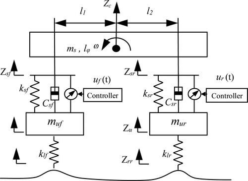
Here it is assumed that the pitch angle φ(t) is small [30], and Equation (1) is obtained based on the following equation: (2) $z_{\mathrm{sf}}\left(t\right)=z_c\left(t\right)-l_1\phi \left(t\right),z_{\mathrm{sr}}\left(t\right)=z_c\left(t\right)+l_2\phi \left(t\right)$(2) In Equation (1), the variables and parameters are listed in Table 1.

Table 1: Half-vehicle active suspension system variables and parameters

Definition of the variable	Symbol	Definition of the parameter	Symbol
Front body displacement	$z_{\mathrm{sf}}\left(t\right)$	Distance between the front axle and the center of mass	$l_1$
Rear body displacement	$z_{\mathrm{sr}}\left(t\right)$	Distance between the rear axle and the center of mass	$l_2$
Front unsprung mass displacement	$z_{\mathrm{uf}}\left(t\right)$	Car body mass	$m_s$
Rear unsprung mass displacement	$z_{\mathrm{ur}}\left(t\right)$	Unsprung mass on the front wheel	$m_{\mathrm{uf}}$
Front terrain height displacement	$z_{\mathrm{rf}}\left(t\right)$	Unsprung mass on the rear wheel	$m_{\mathrm{ur}}$
Rear terrain height displacement	$z_{\mathrm{rr}}\left(t\right)$	Pitch moment of inertia about the center of mass	$I_{\phi }$
Pitch angle	$\phi \left(t\right)$	Stiffness of the passive elements of the front wheel	$c_{\mathrm{sf}}$
Center of mass Displacement	$z_c\left(t\right)$	Stiffness of the passive elements of the rear wheel	$c_{\mathrm{sr}}$
Front actuator force input	$u_f\left(t\right)$	Front tire stiffness	$k_{\mathrm{sf}}$
Rear actuator force input	$u_r\left(t\right)$	Rear tire stiffness	$k_{\mathrm{sr}}$

Based on Equations (1) and (2), the state space representation of the system can be obtained. To do so, the state space variables are defined as $x_1\left(t\right)=z_{\mathrm{sf}}\left(t\right)-z_{\mathrm{ur}}\left(t\right)$ and $x_2\left(t\right)=z_{\mathrm{sr}}\left(t\right)-z_{\mathrm{ur}}\left(t\right)$, which denote the suspension deflections of the front and the rear car body,$x_3\left(t\right)=z_{\mathrm{uf}}\left(t\right)-z_{\mathrm{rf}}\left(t\right)$, $x_4\left(t\right)=z_{\mathrm{ur}}\left(t\right)-z_{\mathrm{rr}}\left(t\right)$, which are the tire deflection of the front and rear car body,$x_5\left(t\right)={\dot{z}}_{\mathrm{sf}}\left(t\right)$, $x_6\left(t\right)={\dot{z}}_{\mathrm{sr}}\left(t\right)$, specifying the vertical velocity of the front and rear car body,$x_7\left(t\right)={\dot{z}}_{\mathrm{uf}}\left(t\right)$,$x_8\left(t\right)={\dot{z}}_{\mathrm{ur}}\left(t\right)$, as the vertical velocity of the front and rear wheels. The control input variables are the front and rear actuator force inputs $u_f\left(t\right)$,$u_r\left(t\right)$ and the disturbance variables are considered as the front and terrain speed, ${\dot{z}}_{\mathrm{rf}}\left(t\right)$,${\dot{z}}_{\mathrm{rr}}\left(t\right)$. The heave and pitch accelerations, ${\ddot{z}}_c\left(t\right)$,$\ddot{\left(t\right)}$ are selected as the performance output variable of the system because the ride comfort, as the main performance criteria, is related to the vertical acceleration experienced by the car body. To guarantee the suspension performance of the designed controller subject to the mechanical constraints of vehicle components and passenger comfort generation, the inequalities of (3) are provided, where $z_{f,\max }$ and $z_{r,\max }$ are the maximum limits for front and rear suspension deflection. (3) $\begin{array}{rl}& |\left(z_{\mathrm{sf}}\right(t)-z_{\mathrm{uf}}(t)|\le z_{f,max}\\ & |\left(z_{\mathrm{sr}}\right(t)-z_{\mathrm{ur}}(t\left)\right)|\le z_{r,max}\end{array}$(3) The following two constraints of (4) are also considered to ensure a firm uninterrupted contact of the wheels with the road. Based on these constraints the dynamic tire loads should not excess the static loads for both front and rear wheel (4) $\begin{array}{rl}& |k_{\mathrm{sf}}\left(z_{\mathrm{uf}}\right(t)-z_{\mathrm{rf}}(t\left)\right)|\le F_f\\ & |k_{\mathrm{sr}}\left(z_{\mathrm{ur}}\right(t)-z_{\mathrm{rr}}(t\left)\right)|\le F_r\end{array}$(4) Here, $F_f$ and $F_r$ are the static tire loads calculated by the following equation: (5) $\begin{array}{rl}& F_r(l_1+l_2)=m_{s}g{l}_1+m_{\mathrm{ur}}g(l_1+l_2)\\ & F_f+F_r=(m_s+m_{\mathrm{uf}}+m_{\mathrm{ur}})\end{array}$(5) By the state space variables, inputs, and the output constraints, the dynamic equations of the HVASS are obtained by the following equation: (6) ${\mathbb{G}}_0:\{\begin{array}{l}\dot{x}\left(t\right)=\mathrm{Ax}\left(t\right)+\mathrm{Bu}\left(t\right)+B_{1}w\left(t\right)\\ z_1\left(t\right)=C_{1}x\left(t\right)+D_{1}u\left(t\right)\\ z_2\left(t\right)=C_{2}x\left(t\right),,x\left(t_0\right)=x_0,w\left(t\right)\in L_2^m\end{array}$(6) where $x\left(t\right)$ is the state vector, $u\left(t\right)$ is the control input vector,$w\left(t\right)$ is the disturbance input and $z_1\left(t\right)$, $z_2\left(t\right)$ are the controlled outputs. Also, x₀ is the initial state vector. The system matrices are defined by the following equation: (7) $\begin{array}{rl}A& =[\begin{array}{cccc}0& 0& 0& 0\\ 0& 0& 0& 0\\ 0& 0& 0& 0\\ 0& 0& 0& 0\\ -a_1{k}_{\mathrm{sf}}& -a_2{k}_{\mathrm{sr}}& 0& 0\\ -a_2{k}_{\mathrm{sf}}& -a_3{k}_{\mathrm{sr}}& 0& 0\\ k_{\mathrm{sf}}/m_{\mathrm{uf}}& 0& -k_{\mathrm{lf}}/m_{\mathrm{uf}}& 0\\ 0& k_{\mathrm{sr}}/m_{\mathrm{ur}}& 0& -k_{\mathrm{lr}}/m_{\mathrm{ur}}\end{array}\\ & \begin{array}{cccc}1& 0& -1& 0\\ 0& 1& 0& -1\\ 0& 0& 1& 0\\ 0& 0& 0& 1\\ -a_1{c}_{\mathrm{sf}}& -a_2{c}_{\mathrm{sr}}& a_1{c}_{\mathrm{sf}}& a_2{c}_{\mathrm{sr}}\\ -a_2{c}_{\mathrm{sf}}& -a_3{c}_{\mathrm{sr}}& a_2{c}_{\mathrm{sf}}& a_3{c}_{\mathrm{sr}}\\ c_{\mathrm{sf}}/m_{\mathrm{uf}}& 0& -c_{\mathrm{sf}}/m_{\mathrm{uf}}& 0\\ 0& c_{\mathrm{sr}}/m_{\mathrm{ur}}& 0& -c_{\mathrm{sr}}/m_{\mathrm{ur}}\end{array}]\\ B& ={\left[\begin{array}{ccccc}{0}_{1\times 4}& a_1& a_2& -1/m_{\mathrm{uf}}& 0\\ 0_{1\times 4}& a_2& a_3& 0& -1/m_{\mathrm{ur}}\end{array}\right]}^T,\\ B_1& ={\left[\begin{array}{ccccc}0& 0& -1& 0& 0_{1\times 4}\\ 0& 0& 0& -1& 0_{1\times 4}\end{array}\right]}^T\end{array}$(7) $\begin{array}{rl}{a}_1& =1/m_s+{l_1}^2/I_{\phi },a_2=1/m_s-l_1{l}_2/I_{\phi },\\ a_3& =1/m_s+{l_2}^2/I_{\phi }\end{array}$ The output matrices of the system are also obtained as given by the following equation: (8) $\begin{array}{rl}{C}_1& =[\begin{array}{cccc}-k_{\mathrm{sf}}/m_s& -k_{\mathrm{sr}}/m_s& 0& 0\\ l_1{k}_{\mathrm{sf}}/I_{\phi }& -l_2{k}_{\mathrm{sr}}/I_{\phi }& 0& 0\end{array}\\ & \begin{array}{cccc}-c_{\mathrm{sf}}/m_s& -c_{\mathrm{sr}}/m_s& c_{\mathrm{sf}}/m_s& c_{\mathrm{sr}}/m_s\\ l_1{c}_{\mathrm{sf}}/I_{\phi }& -l_2{c}_{\mathrm{sr}}/I_{\phi }& -l_1{c}_{\mathrm{sf}}/I_{\phi }& l_2{c}_{\mathrm{sr}}/I_{\phi }\end{array}]\\ C_2& =[\begin{array}{cccc}1/z_{fmax}& 0& 0& 0\\ 0& 1/z_{fmax}& 0& 0\\ 0& 0& k_{\mathrm{sf}}/z_{fmax}& 0\\ 0& 0& 0& k_{\mathrm{sr}}/F_r\end{array}\begin{array}{c}{0}_{1\times 4}\\ 0_{1\times 4}\\ 0_{1\times 4}\\ 0_{1\times 4}\end{array}]\\ D_1& =\left[\begin{array}{cc}1/m_s& 1/m_s\\ -l_1/I_{\phi }& -l_2/I_{\phi }\end{array}\right]\end{array}$(8) For simplicity, the system is reformulated as (9) by considering $z\left(t\right)=\left[\begin{array}{cc}{z}_1\left(t\right)& z_2\left(t\right)\end{array}\right]$ and the matrices defined by $C={\left[\begin{array}{cc}{C}_1& C_2\end{array}\right]}^T,D={\left[\begin{array}{cc}{D}_1& 0\end{array}\right]}^T$. (9) $\mathbb{G}:\{\begin{array}{l}\dot{x}\left(t\right)=\mathrm{Ax}\left(t\right)+\mathrm{Bu}\left(t\right)+B_{1}w\left(t\right)\\ z_1\left(t\right)=\mathrm{Cx}\left(t\right)+\mathrm{Du}\left(t\right)\\ z_2\left(t\right)=C_{2}x\left(t\right),x\left(t_0\right)=x_0,w\left(t\right)\in L_2^m\end{array}$(9)

2.2. Controller Structure

The HVASS controller is assumed to be subject to gain fluctuations and uncertainties. As mentioned earlier, the controller uncertainty may be caused by factors such as buffer size in digital systems, repair of the devices and the aging of the controller components. The controller uncertainty is supposed to have a stochastic source and modeled by a continuous time Markov process. By this assumption, a multi-mode controller gain is considered for the system. The structure of this controller is as the following. (10) $u\left(t\right)=K({\sigma }_t,t)x\left(t\right)$(10) The matrix K(σ_t,t) is the mode-dependent, time-varying controller gain with the compatible dimension, designed to control the system. The parameter {σ_t, t ≥ 0} is the Markov chain governing switching between candidate gains of K(σ_t,t). σ_t, is a continuous-time, discrete-valued Markov process defined in finite set, $\underset{\_}{M}=:\left\{1,2,\cdots ,M\right\}$ with M modes, the initial condition of ${\sigma }_{t_0}={\sigma }_0$ and a generator square matrix in the form of (11). (11) $\begin{array}{rl}& P=\left[p_{\mathrm{mn}}\right],m,n=1,\dots ,M\\ & Pr\left\{{\sigma }_{t+h}=n|{\sigma }_t=m\right\}=\{\begin{array}{ll}{p}_{\mathrm{mn}}h+o\left(h\right)& m\ne n\\ 1+p_{\mathrm{mm}}h+o\left(h\right)& m=n\end{array}\end{array}$(11) Here $p_{\mathrm{mn}}\ge 0$ with the condition of $p_{\mathrm{mm}}=-{\sum }_{n=1,n\ne m}^M{p}_{\mathrm{mn}}$ is the transition rate from mode m of the controller at time t to mode n at time t + h, with h as time increment. To deal with a more practical situation, the controller gain is assumed to include additive norm bounded uncertainty as well. The controller gains of (10) are now defined as $K\left({\sigma }_1,t\right)=\overline{K}\left({\sigma }_t\right)+\mathrm{\Delta K}\left({\sigma }_t,t\right)$ where $\overline{K}\left({\sigma }_t\right)$ is the nominal gain to be designed and $\mathrm{\Delta K}\left({\sigma }_t,t\right)$ is the time-varying, norm-bounded parametric uncertainty.$\mathrm{\Delta K}\left({\sigma }_t,t\right)$ is an unknown, mode-dependent matrix with the following form, (12) $\mathrm{\Delta K}({\sigma }_t,t)=H_K\left({\sigma }_t\right)F_K({\sigma }_t,t)E_K\left({\sigma }_t\right)$(12) where H_K(σ_t) and E_K(σ_t) are known real-valued constant matrices, and F_K (σ_t, t) is unknown time-varying matrix with Lebesgue measurable elements satisfying $F_K^T\left(\sigma ,t\right)F_K\left(\sigma ,t\right)\le I$. Hereafter, for the convenience of notations σ_t= m is used. Thus, matrices are labeled as K(m), ΔK(m,t), E_K(m), H_K(m) and F_K(m, t). Also, for simplicity, the initial time is set to zero, t₀ = 0 and the initial state vector, x₀ and the initial mode, σ₀ are supposed to be available a priory.

3. MAIN RESULTS: ROBUST H₂ GUARANTEED COST CONTROLLER DESIGN

In this section, the controller is assumed to have the mode-dependent state feedback form. Substituting the controller into the system, yields the closed-loop system as (13): (13) $\begin{array}{rl}& {\mathbb{G}}_1:\{\begin{array}{l}\dot{x}\left(t\right)=\overline{A}({\sigma }_t,t)x\left(t\right)+B_{1}w\left(t\right)\\ z\left(t\right)=\overline{C}({\sigma }_t,t)x\left(t\right)\\ x\left(t_0\right)=x_0,\sigma \left(t_0\right)={\sigma }_0,w\left(t\right)\in L_2^m\end{array}\end{array}$(13) (14) $\begin{array}{rl}& \overline{A}({\sigma }_t,t)=A+\mathrm{BK}({\sigma }_t,t),\\ & \overline{C}({\sigma }_t,t)=C+\mathrm{DK}({\sigma }_t,t)\end{array}$(14) Before designing the controller, the following definitions are recalled.

Definition 1:

[31] For any initial mode σ₀, and any given initial state vector x₀, the system ${\mathbb{G}}_1$ with w(t) = u(t) = 0 is said to be robustly stochastically mean square stable (MSS) if (15) $\int E\left\{||x\left(t\right)||\mathrm{dt}|x,\sigma \right\}<\mathrm{\infty }$(15) Holds for all admissible uncertainties, where E {.|.} is the expectation conditioning on the initial distributions of x₀, σ₀.

Definition 2:

[31,32] The H₂ norm of a mean square stable system ${\mathbb{G}}_1$ is defined as: (16) $||{\mathbb{G}}_1|{|}_2^2=\sum _{s=1}^S\sum _{m=1}^M{\mu }_m||z_{s,m}|{|}_2^2$(16) where $z_{s,m}$ represents the output when:

1. The input is given by $w=\left\{w\left(t\right):t\ge 0\right\}$ , $w\left(t\right)=e_s\eta \left(t\right)$ , $\eta \left(t\right)$ is the unitary impulse and$e_s$ the M-dimensional unitary vector formed by 1 at the s^th position and zero elsewhere,

2. $x_0=0$ and $\sigma \left(t\right)=m$ , Clearly, the closed-loop system is a Markov jump linear system and the following lemma provides the stochastic stability with constraint H₂ norm.

Lemma 1:

[32] If there exist square, symmetric, positive definite matrices$P_m$ , such that the following hold for $1\le m\le M:$ (17) $\begin{array}{rl}& {{\overline{A}}_m}^T{P}_m+P_m{\overline{A}}_m+\sum _{n=1}^M{p}_{\mathrm{mn}}{P}_n+{\overline{C}}_m^T{\overline{C}}_m<0,\end{array}$(17) (18) $\begin{array}{rl}& \sum _{m=1}^M{\mu }_m\mathrm{Trace}\left(B_1^T{P}_m{B}_1\right)<\gamma \end{array}$(18) Then the MJLS of $\mathbb{G}{}_0$ is stochastically stable with norm H₂ less than $\sqrt{\gamma }$.

Now the controller can be designed. It is designed such that the resulting closed-loop system is MSS and meets the H₂ performance bound requirement.

Theorem 1:

If there exist symmetric matrices $Q_m,P_m$ and matrices $V_m$ and $L_m$ satisfying the following LMIs for $1\le m\le M:$ (19) $\begin{array}{rl}& [\begin{array}{ccc}-V_m-V_m^T& \ast & \ast \\ A{V}_m+B{L}_m+Q_m& p_{\mathrm{mm}}{Q}_m-Q_m& 0\\ C{V}_m+D{L}_m& 0& -I\\ V_m& 0& 0\\ {\overline{V}}_m& 0& 0\end{array}\\ & \begin{array}{cc}\ast & \ast \\ \ast & \ast \\ \ast & \ast \\ Q_m& \ast \\ 0& -{\overline{Q}}_m\end{array}]<0\end{array}$(19) (20) $\begin{array}{rl}& \sum _{m=1}^M{\mu }_m\mathrm{Trace}\left(B_1^T{P}_m{B}_1\right)<\gamma ,\end{array}$(20) where (21) $\begin{array}{rl}& {\overline{V}}_m^T=[\sqrt{p_{m1}}{V}_m^T\dots \sqrt{p_{m\left(m-1\right)}}{V}_m^T,\\ & \sqrt{p_{m\left(m+1\right)}}{V}_m^T\dots \sqrt{p_{\mathrm{mN}}}{V}_m^T],\end{array}$(21) (22) $\begin{array}{rl}& {\overline{Q}}_m^T=\mathrm{diag}\left[Q_1\dots Q_{m-1}{Q}_{m+1}\dots Q_M\right],\end{array}$(22) Then the suspension system with the form of ${\mathbb{G}}_1$ is stochastically stable with norm H₂ less than $\sqrt{\gamma }$ the controller gains are also obtained by$K_m=L_m{V}_m^{-1}$ .

Proof

1: Consider (14) and (15) as the stability conditions of the closed-loop system with H₂ norm constraint. Select $W_m=-P_{m}A-p_{\mathrm{mm}}{P}_m+P_m$, then (14) can be rewritten in the following form. (23) $\begin{array}{rl}& {\sum }_{n=1,n\ne m}^M{p}_{\mathrm{mn}}P+{\overline{C}}_m^T{\overline{C}}_m-W_m-W_m^T+P_m\\ & -\left(P_m{\overline{A}}_m+W_m\right)(p_{\mathrm{mm}}{P}_m-P_m{)}^{-1}(P_m{\overline{A}}_m+W_m{)}^T\\ & <0,\end{array}$(23) Substitute the closed-loop matrices of (14) into in (20) and the following is obtained: (24) $\begin{array}{rl}& \sum _{n=1,m\ne n}^M{p}_{\mathrm{mn}}{P}_m-W_m-W_m^T+P_m+(C+D{K}_m\\ & +D{H}_{m}F\left(t\right)E_m{)}^T(C+D{K}_m+D{H}_{m}F(t\left)E_m\right)\\ & -\left(P_m(A+B{K}_m)+W_m\right)(p_{\mathrm{mn}}{P}_m-P_m{)}^{-1}\\ & (P_m(A+B{K}_m)+W_m{)}^T<0,1\le m\le M\end{array}$(24) Also, (17) turns to (25) by the Schur complement lemma. (25) $\begin{array}{rl}& \left[\begin{array}{cc}\begin{array}{c}\sum _{n=1,m\ne n}^M(p_{\mathrm{mn}}{P}_n\\ -W_m-W_m^T+P_m^{-1}\\ +{(C+D{K}_m)}^T(C+D{K}_m))\end{array}& \ast \\ P_m(A+B{K}_m)+W_m& p_{\mathrm{mn}}{P}_m-P_m\end{array}\right]<0\\ & 1\le m\le M\end{array}$(25) The inequality $P_m{\overline{A}}_m+\frac{1}{2}{P}_{\mathrm{mm}}{P}_m<0$, $1\le m\le N$ is directly deduced from (14) which leads to $P_m{\overline{A}}_m+P_{\mathrm{mm}}{P}_m-P_m<0$ considering $P_m>0$ and $P_{\mathrm{mm}}<0$. This means that $W_m=-P_i{\overline{A}}_m-P_{\mathrm{mm}}{P}_m+P_m$ is invertible. Define $V_m=W_m^{-1}$ and $Q_m=P_m^{-1}$, pre-multiplying (24) by $\mathrm{diag}\left[V_m^T{Q}_m\right]$ yields (26). (26) $\begin{array}{rl}& [\begin{array}{c}{V}_m^T\left({\sum }_{n=1,n\ne m}^M{p}_{\mathrm{mn}}{Q}_n^{-1}\right)-V_m^T{W}_m-V_m^T{W}_m^T\\ +V_m^T{P}_m+V_m^T{(C+D{K}_m)}^T(C+D{K}_m)\\ \\ Q_m{P}_m(A+B{K}_m)+Q_m{W}_m\end{array}\\ & \begin{array}{c}{V}_m^T{(A+B{K}_m)}^T{P}_m+V_m^T{W}_m^T\\ \\ \\ p_{\mathrm{mm}}{Q}_m{P}_m-Q_m{P}_m\end{array}]<0\end{array}$(26) Post-multiplying (23) by $\mathrm{diag}\left[V_m^T{Q}_m\right]$ provides (27). (27) $\begin{array}{rl}& [\begin{array}{c}{V}_m^T\left({\sum }_{n=1,n\ne m}^M{p}_{\mathrm{mn}}{Q}_n^{-1}\right)V_m-V_m^T{W}_m{V}_m\\ -V_m^T{W}_m^T{V}_m+V_m^T{P}_m{V}_m\\ +V_m^T{(C+D{K}_m)}^T(C+D{K}_m)V_m\\ \\ Q_m{P}_m(A+B{K}_m)V_m+Q_m{W}_m{V}_m\end{array}\\ & \begin{array}{c}{V}_m^T{(A+B{K}_m)}^T{P}_m{Q}_m^T+V_m^T{W}_m^T{Q}_m^T\\ \\ \\ p_{\mathrm{mm}}{Q}_m{P}_m{Q}_m^T-Q_m{P}_m{Q}_m^T\end{array}]<0\end{array}$(27) Via the change in variables by $V_m=W_m^{-1}$ and $Q_m=P_m^{-1},$(26) changes to (28). (28) $\begin{array}{rl}& [\begin{array}{c}{V}_m^T\left({\sum }_{n=1,n\ne m}^M{p}_{\mathrm{mn}}{Q}_n^{-1}\right)V_i-V_m^T-V_m\\ +V_m^T{Q}_m^{-1}{V}_m+V_m^T{(C+D{K}_m)}^T(C+D{K}_m)V_m\\ \\ (A+B{K}_m)V_m+Q_m\end{array}\\ & \begin{array}{c}{V}_m^T{(A+B{K}_m)}^T+Q_m^T\\ \\ \\ p_{\mathrm{mm}}{Q}_m-Q_m\end{array}]<0\end{array}$(28) which can be rewritten in the following form using the following equation: (29) ${\sum }_{n=1,n\ne m}^M{p}_{\mathrm{mn}}{Q}_n^{-1}={\overline{V}}_m^T{\overline{Q}}_m^{-1}{\overline{V}}_m$(29) With further simplifications performed on (28), the inequality of (30) is obtained: (30) $\begin{array}{rl}& [\begin{array}{cc}-V_m-V_m^T& \ast \\ (A+B{K}_m)V_m+Q_m& (p_{\mathrm{mm}}-I)Q_m\\ (C+D{K}_m)V_m& 0\\ V_m& 0\\ {\overline{V}}_m& 0\end{array}\\ & \begin{array}{ccc}\ast & \ast & \ast \\ 0& \ast & \ast \\ -I& \ast & \ast \\ 0& Q_m& \ast \\ 0& 0& -{\overline{Q}}_m\end{array}]<0\end{array}$(30) By defining $K_m{V}_m=L_m$ the LMI of (16) is achieved and the proof is completed.

4. SIMULATION RESULTS

To show the effectiveness and applicability of the proposed theorem, a stabilizing controller is designed in this section and then applied to active suspension system of (6) with the system parameters given at Table 2. The vehicle is assumed to be subject to the velocity disturbance given at Figure 2 for both front and rear wheels. The controller gains are as (31). (31) $\begin{array}{rl}K\left(1\right)& =1\mathrm{e}4\ast \left[\begin{array}{l}\left[\begin{array}{cccc}-\text{9}\text{.40 }& -\text{.611 }& -\text{6}\text{.207 }& \text{.0874 }\\ -\text{1}\text{.83 }& -\text{.2832 }& -\text{.0518 }& -\text{.0487}\end{array}\right]\text{;}\\ \left[\begin{array}{cccc}\text{.426 }& -7.63& -.2493& -5.82\\ \text{.1919 }& -\text{1}\text{.464 }& \text{.0124 }& -\text{.0495}\end{array}\right]\end{array}\right]\\ K\left(2\right)& =1\mathrm{e}4\ast \left[\begin{array}{l}\left[\begin{array}{cccc}-\text{9}\text{.69 }& -\text{.7980 }& -\text{6}\text{.341 }& -\text{.0813 }\\ -\text{1}\text{.82 }& -\text{.3047 }& -\text{.0524 }& -\text{.0504}\end{array}\right]\text{;}\\ \left[\begin{array}{cccc}\text{2}\text{.411 }& -\text{7}\text{.844 }& -\text{.2427 }& -\text{6}\text{.085 }\\ \text{.1882 }& -\text{1}\text{.4425 }& \text{.0125 }& -\text{.0503}\end{array}\right]\end{array}\right]\end{array}$(31) obtained with respect to the assumed uncertainty matrices of (32), (32) $\begin{array}{rl}E\left(1\right)& =E\left(2\right)=[\begin{array}{cccc}-1& -1& -1& -1\\ 2& 2& 2& 2\end{array}\\ & \begin{array}{cccc}1& 1& 1& 1\\ -2& -2& -2& -2\end{array}],\\ H\left(1\right)& =H\left(2\right)=[10;01]\end{array}$(32) and time-varying matrices of $F\left(1\right)=\text{cos}\left(t\right)\mathrm{eye}\left(2\right)$, $F\left(2\right)=\text{sin}\left(t\right)\mathrm{eye}\left(2\right)$ satisfying $F_K^T({\sigma }_t,t)F_K({\sigma }_t,t)\le I.$A realization of the actuator uncertainty by Markov process, σ_t is depicted in Figure 3. It is the result of an uncertainty following the transition rate matrix of $P=\left[-33;2-2\right]$Controlled system states are illustrated in the Figure 4. The output trajectories of the controlled system are illustrated in Figures 5 and 6, respectively. The controller signals are given at Figure 7. The results contain comparisons with the passive suspension system. As the results show, via active controller, despite the disturbance imposed on the system and although there are uncertainties in the controller structure, the system states are successfully converged to their origin. Comparisons between the active and passive control methods also show that the active method is more efficient than the passive schemes in the presence of controller stochastic variations. This superiority is obvious in the settling time required by the two approaches.

Figure 2: Ground velocities disturbances for the front (dashed line) and rear (solid line) wheels

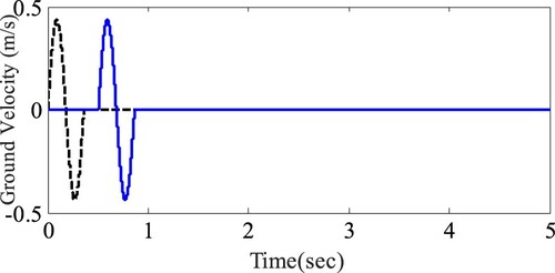
Figure 3: Changing between two modes of the controller

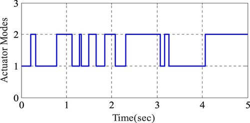
Figure 4: Controlled states of the system

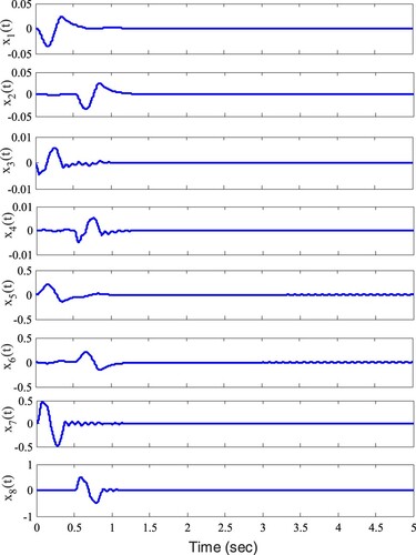
Figure 5: Controlled output z₁(t) = [z₁₁(t), z₁₂(t)]

Figure 6: Controlled outputs z₂(t) = [z₂₁(t), z₂₂(t), z₂₃(t), z₂₄(t)]

Figure 7: Control signal u(t) =[u₁(t), u₂(t)] of the system

Table 2: Parameters of simulated the active suspension system

Parameter	Value	Parameter	Value
$l_1$	1.3 m	$c_{\mathrm{sr}}$	1000 Ns/m
$l_2$	1.5 m	$k_{\mathrm{sf}}$	18.000 N/m
$m_s$	690 kg	$k_{\mathrm{sr}}$	22.000 N/m
$m_{\mathrm{uf}}$	40 kg	$k_{\mathrm{tf}}$	200.000 N/m
$m_{\mathrm{ur}}$	45 kg	$k_{\mathrm{tr}}$	200.000 N/m
$I_{\phi }$	1222 kgm^2	$z_{maxr}$	0.08
$c_{\mathrm{sf}}$	1000 Ns/m	$z_{maxf}$	0.08

5. CONCLUSION

In this paper, robust controller design for an HVASS is discussed in the presence of controller uncertainties. Considering the fact that there is always an inconsistency between the design and implementation of the controller hardware, the controller uncertainty is inevitable. The results show that despite the uncertainties and disturbances, the active suspension system with guaranteed cost control scheme provides an acceptable performance.

However, the proposed structure still faces limitations. Access to the Markov process transition rates is one of the main challenges of the design. An accurate identification of these rates is necessary for the successful implementation of the controller. Therefore, the designed scheme is expected to be extended such that it can consider a more general form of uncertainness in the Markov model of the controller. This is the next step that will be taken by the authors.

Additional information

Notes on contributors

Mona Faraji-Niri

Mona Faraji Niri received her PhD degree in control engineering from Iran University of Science and Technology, Tehran, Iran in 2016. She is currently a research fellow at Warwick Manufacturing Group, The University of Warwick, United Kingdom. Her research interests include electric vehicle dynamics and powertrain modelling and control, battery management systems, stochastic systems, robust control algorithms, and machine learning.

Fatemeh Khani

Fatemeh Khani received her PhD degree in control engineering from Islamic Azad University, Science and Research of Tehran, Iran in 2015. She is currently an assistant professor at Pooyesh Institute of Higher Education, Qom, Iran. Her research interests include optimal control, robust, model predictive control, fault detection and disturbance observers. Email: [email protected]

References

- C. Hua, J. Chen, Y. Li, and L. Li, “Adaptive prescribed performance control of half-car active suspension system with unknown dead-zone input,” Mech. Syst. Signal Process., Vol. 111, pp. 135–48, 2018.
- J. Mrazgua, and M. Ouahi, “Fuzzy fault-tolerant H∞ control approach for nonlinear active suspension systems with actuator failure,” Procedia. Comput. Sci., Vol. 148, pp. 465–74, 2019.
- S. B. A. Kashem, M. Ektesabi, and R. Nagarajah, “Comparison between different sets of suspension parameters and introduction of new modified skyhook control strategy incorporating varying road condition,” Veh. Syst. Dyn., Vol. 50, no. 7, pp. 1173–90, 2012.
- P. S. Els, J. N. J. Theron, P. E. Uys, and M. J. Thoresson, “The ride comfort vs. handling compromise for off-road vehicles,” J. Terramechanics, Vol. 44, no. 4, pp. 303–17, 2007.
- W. Sun, H. Pan, Y. Zhang, and H. Gao, “Multi-objective control for uncertain nonlinear active suspension systems,” Mechatronics, Vol. 24, no. 4, pp. 318–27, 2014.
- X. Shao, F. Naghdy, H. Du, and H. Li, “Output feedback H∞ control for active suspension of in-wheel motor driven electric vehicle with control faults and input delay,” ISA Trans., Vol. 92, pp. 94–108, 2019.
- J. Marzbanrad, and N. Zahabi, “H∞ active control of a vehicle suspension system exited by harmonic and random roads,” Mech. Mech. Eng., Vol. 21, no. 1, pp. 171–180, 2017.
- N. M. Ghazaly, A. E. N. S. Ahmed, A. S. Ali, and G. T. El-Jaber, “H∞ control of active suspension system for a quarter Car model,” Int. J. Veh. Struct. Syst., Vol. 8, no. 1, pp. 14519–14524, 2016.
- K. D. Rao, and S. Kumar. “Modeling and simulation of quarter car semi active suspension system using LQR controller,” In 3rd International Conference on Frontiers of Intelligent Computing: Theory and Applications (FICTA) 2014. Springer, Cham, 2015, pp. 441–8.
- R. Kalaivani, P. Lakshmi, and K. Sudhagar, “Vibration control of vehicle active suspension system using novel fuzzy logic controller,” Int. J. Enterpr. Netw. Manage., Vol. 6, no. 2, pp. 139–52, 2014.
- Z. Xie, P. K. Wong, J. Zhao, and T. Xu, “Design of a denoising hybrid fuzzy-pid controller for active suspension systems of heavy vehicles based on model adaptive wheelbase preview strategy,” J. Vibroeng., Vol. 17, no. 2, pp. 883–904, 2015.
- H. Li, X. Jing, and H. R. Karimi, “Output-feedback-based H∞ control for vehicle suspension systems with control delay,” IEEE Trans. Ind. Electron., Vol. 61, no. 1, pp. 436–46, 2013.
- H. Li, H. Liu, S. Hand, and C. Hilton, “Design of robust H∞ controller for a half-vehicle active suspension system with input delay,” Int. J. Syst. Sci., Vol. 44, no. 4, pp. 625–40, 2013.
- W. Sun, H. Pan, J. Yu, and H. Gao, “Reliability control for uncertain half-car active suspension systems with possible actuator faults,” IET Control Theory Applic., Vol. 8, no. 9, pp. 746–54, 2014.
- M. Moradi, and A. Fekih, “Adaptive PID-sliding-mode fault-tolerant control approach for vehicle suspension systems subject to actuator faults,” IEEE Trans. Veh. Technol., Vol. 63, no. 9, pp. 1041–54, 2013.
- H. Du, J. Lam, and K. Y. Sze, “Design of non-fragile H∞ controller for active vehicle suspensions,” J. Vib. Control, Vol. 11, no. 2, pp. 225–43, 2005.
- H. Du, J. Lam, and K. Sze, “Non-fragile output feedback H∞ vehicle suspension control using genetic algorithm,” Eng. Appl. Artif. Intell., Vol. 16, pp. 667–80, 2003.
- H. Li, H. Liu, C. Hilton, and S. Hand, “Non-fragile H∞ control for half-vehicle active suspension systems with actuator uncertainties,” J. Vib. Control, Vol. 19, no. 4, pp. 560–75, 2013.
- G. Wang, C. Chen, and S. Yu, “Robust non-fragile finite-frequency H∞ static output-feedback control for active suspension systems,” Mech. Syst. Signal. Process., Vol. 91, pp. 41–56, 2017.
- Y. Kong, D. Zhao, B. Yang, C. Han, and K. Han, “Non-fragile multi-objective static output feedback control of vehicle active suspension with time-delay,” Veh. Syst. Dyn., Vol. 52, no. 7, pp. 948–68, 2014.
- Y. Kong, D. Zhao, B. Yang, C. Han, and K. Han, “Robust non-fragile H∞/ L2− L∞ control of uncertain linear system with time-delay and application to vehicle active suspension,” Int. J. Robust Nonlinear Control, Vol. 25, no. 13, pp. 2122–41, 2015.
- M. Faraji-Niri, M. R. Jahed-Motlagh, and M. Barkhordari-Yazdi. “Robust stabilization of uncertain non-homogeneous Markov jump linear systems,” The 3rd International Conference on Control, Instrumentation, and Automation, 2013, pp. 42–6.
- M. Faraji-Niri, M. R. Jahed-Motlagh, and M. Barkhordari-Yazdi, “Stochastic stability and stabilization of a class of piecewise-homogeneous Markov jump linear systems with mixed uncertainties,” Int. J. Robust Nonlinear Control, Vol. 27, no. 6, pp. 894–914, 2017.
- K. Shi, J. Wang, Y. Tang, and S. Zhong, “Reliable asynchronous sampled-data filtering of T–S fuzzy uncertain delayed neural networks with stochastic switched topologies,” Fuzzy Sets Syst., Vol. 381, pp. 1–25, 2020.
- K. Shi, J. Wang, S. Zhong, Y. Tang, and J. Cheng, “Non-fragile memory filtering of TS fuzzy delayed neural networks based on switched fuzzy sampled-data,” control,” Fuzzy Sets Syst., Vol. 394, pp. 40–64, 2020.
- Y. Xu, M. Fang, Y. J. Pan, K. Shi, and Z. G. Wu, “Event-triggered output synchronization for nonhomogeneous agent systems with periodic denial-of-service attacks,” Int. J. Robust Nonlinear Control, Vol. 31, pp. 1851–1865, 2020.
- K. Shi, Y. Tang, X. Liu, and S. Zhong, “Non-fragile sampled-data robust synchronization of uncertain delayed chaotic Lurie systems with randomly occurring controller gain fluctuation,” ISA Trans., Vol. 66, pp. 185–99, 2017.
- K. Shi, Y. Tang, S. Zhong, C. Yin, X. Huang, and W. Wang, “Nonfragile asynchronous control for uncertain chaotic Lurie network systems with Bernoulli stochastic process,” Int. J. Robust Nonlinear Control, Vol. 28, no. 5, pp. 1693–714, 2018.
- K. Shi, J. Wang, S. Zhong, X. Zhang, Y. Liu, and J. Cheng, “New reliable non-uniform sampling control for uncertain chaotic neural networks under Markov switching topologies,” Appl. Math. Comput., Vol. 347, pp. 169–93, 2019.
- H. Du, and N. Zhang, “Constrained H∞ control of active suspension for a half-car model with a time delay in control,” Proc. Inst. Mech. Eng., Part D: J. Automobile Eng., Vol. 222, no. 5, pp. 665–84, 2008.
- E. K. Boukas. Stochastic switching systems: analysis and design. Basel: Birkhäuser, 2005.
- D. P. De Farias, J. C. Geromel, J. B. Do Val, and O. L. V. Costa, “Output feedback control of Markov jump linear systems in continuous-time,” IEEE Trans. Autom. Control, Vol. 45, no. 5, pp. 944–9, 2000.