Recommendations for riparian buffer widths based on field surveys of erosion processes on steep cultivated slopes

Abstract

Results of field surveys are used to build knowledge about erosion processes occurring on steep cultivated slopes next to watercourses, and to propose conservation measures with an emphasis on widths for riparian buffer strips. The surveys were conducted on a 108-km² watershed in Portneuf region, Québec, Canada. Using a handheld global positioning system (GPS), measuring tapes, a 0.5-m resolution satellite image and a 1-m resolution Digital Terrain Model (DTM), 12 erosion-prone areas, totalling 53 ha, located close to river banks were surveyed during four days of the rainy and snowmelt period of April–May 2012. As a result, 328 erosion features were identified and classified into 10 categories. Predominant erosion features included rills, ephemeral gullies and sheet erosion (70% of all features observed). Rills and smaller gullies had lengths of 0.5–160 m, depths of 5–55 cm, and breadths of 5–130 cm. Most erosion features (n = 194) occurred on hillslopes > 8% and had lengths of 10–60 m. At present, most riparian buffer strips in the surveyed field are 1–3 m wide, which is the minimum dimension required by the provincial policy that regulates vegetated filters. In most places surveyed, ephemeral gullying on steep slopes simply extends through the thin 1–3 m buffer strip to easily discharge sediments and pollutants into flowing streams. Based on the local slopes assessed, it is proposed herein to convert these steep cultivated hillslopes into riparian buffer strips of 10–60 m, so that vegetated strips effectively act as boundaries between watercourses and damaging uphill erosion processes, which are sources of sedimentation and, in all likelihood, eutrophication.

Résumé

Dans le présent projet, des relevés terrain ont été réalisés afin d’étudier les processus d’érosion sur des pentes cultivées proches des cours d’eau, et de proposer des mesures de conservation, particulièrement les largeurs des bandes riveraines. Les relevés terrain ont été faits dans un bassin versant de 108 km2 dans la région de Portneuf, Québec, Canada. En utilisant un GPS (global positioning system) de poche, des rubans à mesurer, une image satellitaire à 0.5 m résolution et un modèle numérique de terrain (MNT) à 1 m résolution, 12 zones assujetties à l’érosion (totalisant 53 ha) et situées proches des cours d’eau ont été relevées pendant quatre journées durant la période de fortes pluies et de fonte de neige des mois d’avril–mai 2012. Le résultat est 328 traces d’érosion relevées et classées en 10 catégories. Les érosions prédominantes sont l’érosion en nappe et les ravinements au champ (70% de toute l’érosion observée). Les ravinements avaient des longueurs de 0.5–160 m, des profondeurs de 5–55 cm, et des largeurs de 5–130 cm. La plupart des traces d’érosions (n = 194) se produisent sur des pentes > 8% et ont des longueurs de 10–60 m. à l’heure actuelle, les bandes riveraines sur le terrain sont de 1–3 m, le minimum requis pour se conformer à la politique provinciale réglementant la largeur des bandes riveraines. Dans la plupart des zones relevées, le ravinement se fait tout simplement à travers la mince bande riveraine de 1–3 m pour aisément aller déposer les sédiments et polluants dans le cours d’eau. Sur la base des pentes évaluées, il est proposé dans cet article de convertir ces pentes cultivées en bandes riveraines de 10–60 m, de sorte que la bande de végétation agisse comme un tampon entre le cours d’eau et les cicatrices découlant du processus d’érosion en amont (en tant que sources de sédimentation et possiblement d’eutrophisation).

Introduction

The ability to synthesize knowledge from a wide range of fields to inform policy and decision-making is one of the key challenges to a successful environmental management framework. Leaving aside the potential for politicization of science (e.g., Lackey 2007; Irvine 2009), translating scientific principles into environmental management policies and practices remains a daunting challenge, frequently testing the limits of expert knowledge (see e.g., Boardman 2006 and Bui et al. 2011). The field of soil erosion assessment faces this challenge too when it comes to implementing results into conservation policy definition (e.g., Stonehouse and Bohl 1993; Renschler and Harbor 2002; Knowler and Bradshaw 2007).

Nonetheless, in the twenty-first century, soil erosion remains a major land degradation problem (Lal 2001), and the ensuing impact seems to be receiving renewed interest internationally (e.g., Prasuhn 2011; Liu et al. 2012). Erosion is a natural hazard, but it can be exacerbated by human activities. Using data drawn from a global compilation of studies, Montgomery (2007) quantitatively confirmed the long-articulated contention that erosion rates from conventionally plowed agricultural fields are, on average, one to two orders of magnitude greater than rates of soil production, erosion under native vegetation and long-term geological erosion.

The consequences of accelerated erosion on agricultural lands are two-fold: (1) on-site, loss of fertile topsoil threatens to decrease agricultural production, and (2) off-site, delivery of eroded sediments and adsorbed contaminants can pollute waterways and receiving water bodies (Lal 2001). In Canada, soil erosion is a major threat to the sustainability of agriculture because it decreases potential storage volume of water for crops, reduces the total nutrient supply, threatens soil structure and tilth (Lobb et al. 2010), and causes significant off-farm adverse environmental impacts through the release of nutrients, pesticides, pathogens and toxins, particularly in water bodies (Gordon et al. 2011; Rees et al. 2011). Moreover, the presence of eroded fine sediments in watercourses can have negative impacts on biodiversity. For example, in Québec, deposited fine sediments are reported to kill spawns or damage spawning grounds (Avery et al. 2011).

A solution to the off-site impacts of soil erosion is the implementation of riparian buffer strips, which when composed of native or planted vegetation can remove sediments and other pollutants from surface runoff by filtration, deposition, infiltration, adsorption, absorption, decomposition and volatilization (Dillaha et al. 1989; Nieswand et al. 1990; P.M. van Dijk et al. 1996; Gumiere et al. 2011). In this way, the riparian buffer strip becomes the boundary that lies between the watercourse and damaging uphill erosion processes (as sources of sedimentation and potential eutrophication).

In the province of Québec, Canada, there exists a prototype two-dimensional (2D) landform used as the basis for regulating the minimum vegetated riparian buffer width (Ministère du développement durable de l’environnement et des parcs [MDDEP] 2007a, 2007b, 2007c). The basis is to keep a buffer strip of 10 or 15 m from the high water level line (Provincial Regulation, LRQ c. Q-2, r. 35, ar. 2.2), but the regulation becomes lenient when allowing cultivations at a minimum of 3 m from the high water line or at a 1-m buffer from the embankment (Provincial Regulation, LRQ c. Q-2, r. 35, ar. 3.3-f). In discussing possible riparian buffer widths suitable for Québec, Gagnon and Gangbazo (2007) recognized that a single range of optimum widths would not be possible as buffer width depends on topography, soil type, hydrological processes, etc., and that based on 12 studies worldwide, optimum widths recommended for vegetated filters buffering uniform shallow flow can vary between 7.5 m wide (mean of 15 m) to 114 m wide (mean of 68 m).

While erosion modelling exercises can provide insight into beneficial management practices (BMPs) or optimum riparian buffer widths to be adopted (e.g., Michaud et al. 2007; Rousseau et al. 2012, 2013; Gumiere et al. 2013), field surveys supported by geospatial analysis represent a complementary approach for smaller areas (e.g., Jankauskas and Fullen 2002; Dosskey et al. 2005; van Dijk et al. 2005).

It is generally recognized that four factors affect erosion, namely, rainfall, soil type, topography, and land cover type and practices (e.g., the RUSLE-CAN model by Wall et al. 2002). On individual undulating land parcels, three of the following four factors can be constant: rainfall depth, soil type and land cover type and practices (Wischmeier and Smith 1978; Renard et al. 1997). This leaves topography as the only variable factor for active erosion processes taking place on such sites (Shi et al. 2012). With recent advances in satellite remote sensing technologies, it is possible to obtain high-resolution digital terrain models (DTM) every 1–2 days for an area of interest (e.g., Anderson and Marchisio 2012). With such DTMs and field GPS erosion surveys, it is possible to build a detailed Geographic Information System (GIS) database depicting observed erosion features and the slope steepness and length (LS) factor to understand erosion processes occurring and to propose conservation measures.

The present study aims to build knowledge about field erosion processes occurring on steep cultivated slopes next to watercourses and to propose conservation measures, particularly adequate widths for riparian buffer strips. The following steps are applied to achieve this goal, namely: (1) perform a GPS-based field survey of erosion features on erosion-prone hillslopes of a selected watershed, (2) classify and categorize the erosion features observed, (3) analyse geospatially the results with respect to soil type and use, hydrological processes in place, and topography (1-m DTM derived from remote sensing), and (4) analyse the different kinds of three-dimensional (3D) complex landforms existing in the field and being degraded by erosion, while impacting downslope water bodies by passing through vegetated filters. Based on landforms observed, conservation measures can be proposed. It is postulated in this work that the real 3D landscapes are not properly taken into account in the current prototype 2D landform implemented in current regulation (MDDEP 2007a). Consequently, this lack of accounting for complex 3D landforms in the regulation may result in an inadequate protection of watercourses and water bodies against uphill erosion processes.

Study area description

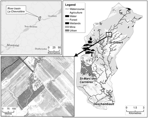
The study area is a small, 108-km², watershed (Figure 1) located (72°0’W, 46°43’N) in the Portneuf municipal region of Québec. The source of the Chevrotière River is situated in the town of Sainte-Christine d’Auvergne in a wetland environment and it discharges in the St. Lawrence River between the towns of Deschambault and Grondines. The Chevrotière River is about 29 km long with an average slope of about 1% (La Corporation d’aménagement et de protection de la rivière Sainte-Anne [CAPSA] 2011).

Figure 1 The study area, La Chevrotière watershed (108 km²) situated in the province of Quèbec, Canada. The main economic activity within the watershed is agriculture (crop production, beef production and dairy), which covers 34% of the watershed surface area.

The geological formations are the Grenville for the northern part (1.2 GY to 950 MY) and the Plate-forme du Saint-Laurent (700–350 MY) for the southern part. The Grenville consists of a variety of igneous and sedimentary rocks that have undergone strong deformation and are metamorphosed. The Plate-forme du Saint-Laurent stratum is composed of sedimentary rocks lying on top of formations from the Grenville (Bourque 2004; Ministère des Ressources naturelles et de la Faune [MRNF] 2006).

Regarding topography, the watershed starts at the northern bank of the St. Lawrence River to reach an elevation of 150 m in the interior. Based on calculated slopes with a 1-m resolution DTM, 40% of the watershed has slopes < 2% (∼3°) and 47% of the watershed has slopes between 2–8% (∼3–9°). Most of the landscape is either farmed or covered by forest and urban areas. At stream locations, the flat terrain becomes undulated with slopes > 8%, that are being exploited for farming, forest and shrubs.

Soils present in the watershed belong to the following five taxonomic orders (Figure 2) (Agriculture and Agri-Food Canada [AAFC] 2010):

• Brunisols (soils formed under forest cover, ideal for agricultural production),

• Gleysols (waterlogged soils, limited agricultural production),

• Podzols (soils formed on acid parent materials under forest vegetation),

• Regosols (sandy soils with poorly developed drainage), and

• Organic (soils saturated with water for prolonged periods).

Figure 2 Soil map of the watershed (see text for description of soil types).

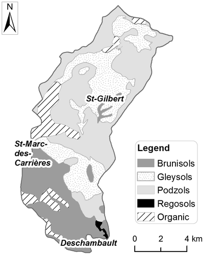
The soils are mostly clayey (St-Gilbert), coarse-loamy textured (in St-Marc-des-Carrières and Deschambault), and sandy (around St-Gilbert). Drainage classes are in four categories ranging from moderately well drained to poorly drained soils. In the region of interest, namely St-Gilbert and St-Marc-des-Carrières, farming takes place mostly on imperfectly, poorly and very poorly drained soils (Ministère de l’Agriculture, des Pêcheries et de l’Alimentation du Québec [MAPAQ] and Institut de recherche et de développement en agroenvironnement [IRDA] 2003).

Climate, hydrology and land use

The climate in the watershed is humid continental. There are significant temperature variations, with hot summers, cold winters and abundant rainfall. Average annual temperatures range from 4.2–5.8°C. Average annual precipitation recorded at the Deschambault station (period 1976–2006) is 1132 mm (Standard Deviation [SD] = 88 mm), with a mean annual rainfall of 932 mm (SD = 89 mm) (Environment Canada [EC] 2007). The month with the highest rainfall amount is July with a mean of 125 mm and SD = 28 mm (Table 1).

Table 1. Mean monthly rainfall (1976 to 2006) from April to October at Deschambault station (Lat 46°41’27”N, Long 71°58’18”W). Data source: EC (2007).

Month	Rainfall depth (mm)
	Mean	SD	Min	Max
April	73	25	7	154
May	101	34	29	233
June	109	31	33	221
July	125	28	55	224
August	109	25	31	181
September	120	28	60	225
October	100	21	36	159

The average daily discharge (2006–2010) near the river outlet is 0.35 m³ s^–1, with the month of April having the largest average daily flow (1.15 m³ s^–1, period 2006–2010) (MDDEP and Centre d’expertise hydrique du Québec [CEHQ] 2011). As shown in Table 1, although April is not the month with the highest rainfall of the year, it is nonetheless the month where river flow and surface runoff are highest, and this is due to snowmelt and saturated soil conditions. During this period, high runoff combined with little vegetative cover produce erosion. Regarding land use, the main economic activity of the watershed is agriculture (crop production, beef production and dairy), which covers 34% of the watershed. Forest cover is 60%. The rest comprises urban areas (5%), and water bodies and wetlands (1%) (see Figure 1) (CAPSA 2011).

Erosional areas of the watershed and existing regulations

During the preliminary description of the watershed performed by CAPSA (the organisation in charge of the integrated water resources management in the watershed), some 50 erosional areas were identified (covering all types of erosion – sheet and rill, erosion, bank erosion, etc.), including a dozen areas that are steep cultivated hillslopes close to streams (CAPSA 2011). For many of these agricultural sites, CAPSA had started planting herbaceous, shrubby and arboreous species along the riparian zone. Additionally, in a few instances, steep hillslopes had been converted into riparian buffer strips (in collaboration with the land owners), which is an example of the possibility to extend uphill vegetated filters for water protection.

Currently, the provincial government follows its policy Protection of riverbanks, littoral zones and floodplains to protect rivers and lakes against pollution and environmental damage (MDDEP 2007a). In agricultural areas, the riparian buffer width must be at least 3 m beyond the high water line or 1 m above the embankment. In addition, the Environmental regulation on agricultural farms (REA) regulates the application of fertilizers in the field in order to reduce downstream impacts (MDDEP 2002).

Materials and methods

GIS database and remote sensing images of the watershed

A GIS database was created for the watershed including: a Digital DTM, a pair of stereoscopic satellite images and auxiliary data obtained from CAPSA, such as soil, cadastral data, infrastructure, etc. The GIS projection is MTM7 (Modified Transverse Mercator, 7), with the North American Datum – NAD 1983. The GIS database was designed for the study of erosion features surveyed in the field, notably their soil types and topographic slopes.

The satellite imagery characterizes bare soil following snowmelt and was captured by the satellite Worldview2 over the watershed on 14 April 2012 at 15:58 and 15:59 GMT. Each image has eight multispectral bands at 2-m spatial resolution and one panchromatic band at 0.5-m resolution. The captured images, which were in UTM projection with WGS84 datum, were geo-referenced to fit with the GIS database projection.

The stereoscopic image pair was used to generate a 1-m DTM that was contracted to Effigis Inc. One of the images (captured at 15:58 GMT) was pansharpened to generate a high-resolution image with eight multispectral bands at 0.5-m resolution. Pansharpening is the process of fusing a high-resolution panchromatic image with a lower-resolution multispectral image. The pansharpening was done with the software PCI geomatics (PCI Geomatics Enterprises 2011).

Field erosion survey

A first visit to the erosion zones was made on 20 April 2012 together with CAPSA personnel. Low rainfall was experienced on that day and the days that followed:

1. Friday, 20 April: 6.5 mm of rainfall

2. Saturday, 21 April: 14 mm (+1.0 mm of snow)

3. Sunday, 22 April: 22.8 mm

4. Monday, 23 April: 22.3 mm

Previously, rainfall occurred on 10 and 11 April (7.4 and 1.0 mm, respectively). Rainfall more or less ceased on Tuesday, 24 April, and the surveys began. Figure 3 shows the rainfall recorded at the Deschambault station and flow in the Chevrotière River, before and during the survey period (data from EC 2012a and MDDEP and CEHQ 2012).

Figure 3 Rainfall and river flow before and during the survey period. Data source: EC (2012b), MDDEP and CEHQ (2012).

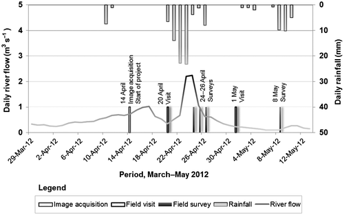
As shown in Figure 3, the most significant erosive rainfall events during the month of April occurred during the period 20–23 April. The surveys started after that date (on 24 April). The river flow follows the same pattern as rainfall, with a maximum flow of 2.24 m³ s^–1 on 24 April. The field surveys were conducted between 24 and 26 April. New erosion zones were then visited with CAPSA on 1 May; the zones were then surveyed on 8 May. In total there were four days of intensive surveys. Equipment used during the survey included measuring tapes (3 m and 50 m long), a portable GPS, a notebook for sketching and a digital photographic camera with video. During the field survey the following characteristics were noted:

• GPS coordinates and lengths of visible erosion features;

• Depth and width of different segments along each erosion feature;

• Drawings, sketches and categorization of the observed erosion features (a detailed description of the categorization scheme used is discussed below); and

• Micro-topography and landscape next to erosion features using photographs and videos.

In total, 12 erosion zones were surveyed: one zone near Deschambault, another in St-Marc-des-Carrières, and the remaining in St-Gilbert. These zones are recognized by CAPSA as being affected by soil erosion. All zones (53 ha) are farmed and are located near river banks. They had mostly bare tilled soil when surveyed (or with little vegetation), except for zones 3, 4, 5 and 6, where large portions of the land are covered by pasture (Figure 4 and Table 2).

Figure 4 The 12 erosion zones surveyed.

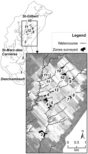
Table 2. Characteristics of each erosion zone visited (see Figure 4).

Zone		Slope (%)	Soil
No.	Area (ha)		Status	Use	Texture	Drainage	Soil Series^q	Order
1	4.7	2–8% and 8–13% (towards the bank)	Bare - tilled	Maize culture	Coarse loamy	good	Fa	Brunisols
					Sandy	imperfect	J	Podzols
2	1.3	2–8% and 6–10% (bank)	Bare - tilled	culture	Coarse loamy	good	Ba	Brunisols
3	9	> 8%	Not tilled	culture fodder	Sandy	imperfect	Ac	Podzols
4	6.7	2–8% on the flat part & > 8% (towards the bank)	Bare - tilled	culture	Coarse loamy	imperfect	Ce	Gleysols
5	3.2		Not tilled	pasture
6	3.1		Tilled in east, west	pasture bare soil	Clayey	good	Ri-e	Gleysols
7	4.1		Not tilled	culture fodder	Loam	good	Pc	Brunisols
8	0.6
9	3.3		Bare - tilled & grass	culture & pasture	Clayey	good	Ri-e	Gleysols
10	13		Bare - tilled	culture	Coarse loamy	imperfect	Ce	Gleysols
11	2.6		Not tilled	culture	Clayey	good	Ri-e	Gleysols
12	1.1		Bare - tilled	culture

^qSoil series: Fa, Farmington; Ba, Batiscan; Pc, Pontiac; Ce, Chaloupe; Ri-e, Rideau; J, Saint-Jude; Ac, Achigan.

Survey data processing

Six hundred and sixty three photos and 12 videos were taken in the field to analyse the erosion features surveyed. These photos and videos were geo-referenced in the GIS database using the following procedure:

1. The photo was first inspected.

2. At the place where the photo was taken, a GPS point was also noted.

3. The time the photo was taken (hh: mm: ss) corresponds to the time that the GPS point was recorded.

4. By establishing an automatic relationship between the two times, it is possible to automatically position the photo on the satellite imagery.

5. Often, a GPS point recorded was not always exactly at the place it should have been because the handheld GPS used had an accuracy of a few metres.

6. The GPS point in question was, when needed, shifted by a few metres in order to match as closely as possible the real location. Elements on the image and corresponding elements on the photograph helped during this step, such as corners of trees, curves of the river, crossing ditches and even traces of erosion.

7. Once the location where the photograph was taken was identified, the next step was to define the field of view of the photograph in the form of a semi-triangular polygon pointing in the direction the photo was taken.

8. After the semi-triangular polygon was created, the photo was attached to the polygon using the hyperlink tool. In the present case, the GIS software used was ArcGIS10 (Environmental System Research Institute [ESRI] 2010).

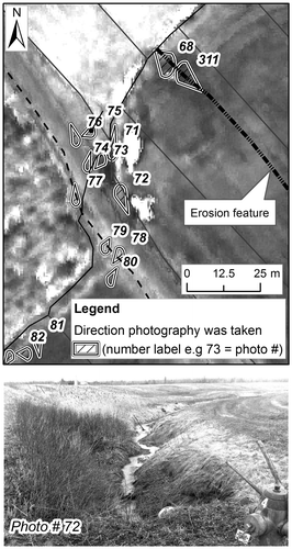
Figure 5 shows some of the semi-triangular polygons created, to which photos were hyperlinked. By clicking on the polygon in the GIS, the hyperlinked photo automatically appears on the screen. One such photo, #72, is shown in Figure 5 (note: the region shown corresponds to the middle of the inset of Figure 1).

Figure 5 Geo-referencing of photographs.

After the GPS points and photographs were geo-referenced in the GIS, it was possible to digitize the surveyed erosion features. For this, the sketches and drawings, as well as the measurements (length, width and depth) that had been made in the field were digitized and geo-referenced in the GIS.

Categorization of erosion features

A fact sheet on the diagnosis and solutions to erosion problems in the field has been devised by Agriculture and Agri-Food Canada (AAFC) and the Ministère de l’Agriculture, des Pêcheries et de l’Alimentation du Québec (MAPAQ). The factsheet elaborates on six categories of erosion commonly observed in the field (AAFC and MAPAQ 2007). These six categories were also observed in the present study and were thus adopted:

1. Interrill or sheet erosion – uniform or non-concentrated flow of water that detaches and transports soil particles. Particles detached from sheet erosion are often later transported in rills.

2. Ephemeral field gullying – detachment and transport of soil particles by a concentrated flow of water. Ephemeral gullies more or less occur at the same place each year and can be obliterated by tillage. When smaller in size and occurring at any location (haphazardly), such gullies should be called rills (rill erosion). When ephemeral gullies cannot be obliterated by tillage (thus becoming permanent), they are called classical gullies.

3. Erosion at confluences – confluences of ditches, runnels and furrows are often prone to erosion, since runoff volume and flow are significant in these spots.

4. Poor drainage of depressions – when depressions filled with water start to drain in an uncontrolled manner, thereby causing gullying problems.

5. Resurgence of subsurface runoff or unconfined groundwater – when water resurges in steep hillside and causes gullying, especially if the soil is tilled and bare.

6. Bank erosion – like confluences, banks of watercourses are zones where risk of erosion is high, because of concentration of surface runoff and differences in elevation between fields and watercourses.

In addition to the above six categories, two other types of erosion were observed in the field, and were thus added to the list, namely:

1. Tunnel erosion – water seeps through subsoil forming underground channels (e.g. Zhu 2012). The process begins on cultivated lands and finishes in the lower part of the bank over lengths of 3–13 m. Causes of tunnel erosion observed in the field are due to poor vegetation cover, sheet and gully erosion upslope, and the presence of a steep slope that increases concentrated runoff.

2. Erosion due to malfunctioning drainage sumps – when the capacity of the sump (also known as a drainage well) to evacuate water is exceeded or the sump is clogged with sediments, there is an overflow of water that makes its way to the watercourse via the surface, thereby causing erosion.

Furthermore, inspired by the work of Deslandes and Belvisi (2008), the abovementioned category 2 (ephemeral field gullying or rill erosion) was expanded to create two additional categories:

1. Ephemeral field gullying connected to stream – when concentrated flowing water with high kinetic energy detaches and transports soil particles towards riparian buffer strips and goes through it to reach the stream.

2. Ephemeral field gullying connected to ditches – when concentrated flowing water detaches and transports soil particles towards man-made ditches and drains.

In the field, the biggest difference between these two categories was that gullying connected to streams had much steeper slopes than gullying connected to ditches. With these two new categories, category 2 was restricted to small ephemeral field gullying alone (i.e. rill erosion).

Results

Figure 6 illustrates the abovementioned erosion categories as observed in the field. The total number of erosion features surveyed was 328, with a total length of 8206 m, including indicative lengths of sheet erosion observed (Table 3). Ephemeral field gullying connected to stream was most common, followed by sheet erosion and rill erosion. Rills and ephemeral gullies had individual lengths of 0.5–160 m, depths of 5–55 cm, and breadths of 5–130 cm. It must be noted that the number and length for sheet erosion features is only indicative of the occurrence of this erosion category in the field. Sheet erosion is the only one of the 10 erosion categories identified above to not produce linear traces. In fact, sites affected by sheet erosion were identified by the deposition of eroded material in the downstream ledges, or near the bank. In this case, the “length” of the sheet erosion that occurred was obtained by measuring the segment from where the sheet erosion began to where the materials were deposited.

Figure 6 Different erosion categories surveyed.

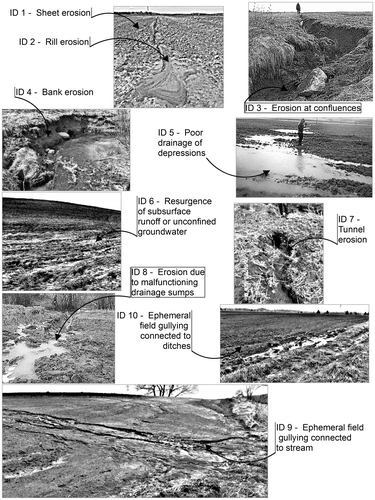
Table 3. Erosion categories ranked according to total length surveyed.

Rank	Erosion category	ID	Number of features n	Total length L (m)
1^st	Ephemeral field gullying connected to stream	9	38	1983 (mean = 52, SD = 40)
2^nd	Sheet erosion	1	99	1832 (mean = 19, SD = 16)
3^rd	Rill erosion	2	83	1566 (mean = 19, SD = 19)
4^th	Poor drainage of depressions	5	23	788 (mean = 34, SD = 49)
5^th	Resurgence of subsurface runoff or unconfined groundwater	6	26	508 (mean = 20, SD = 12)
6^th	Erosion due to malfunctioning drainage sumps	8	10	488 (mean = 49, SD = 29)
7^th	Erosion at confluences	3	16	454 (mean = 28, SD = 46)
8^th	Ephemeral field gullying connected to ditches	10	10	359 (mean = 36, SD = 19)
9^th	Bank erosion	4	7	127 (mean = 18, SD = 5)
10^th	Tunnel erosion	7	16	101 (mean = 6, SD = 12)
Total			328	8206

Table 4 gives the number and length of the different erosion categories observed in each zone visited. Category 1, sheet erosion, was observed in all zones except zone 5, where the site is used for pasture. Category 9, ephemeral field gullying connected to stream, occurred everywhere, except for zone 10, where water was evacuated from the field by drainage sumps installed onsite. In four locations, these sumps failed to work properly, resulting in erosion due to malfunctioning drainage sumps (see row ID 8, Table 4). Rill erosion was also very common, except in zones 5 and 6, where there were pastures and processes of ephemeral field gullying connected to stream, respectively (Table 2 gives a description of each zone surveyed). The zone with the greatest number of features (in terms of length) was zone 7 (l = 1355 m, n = 39). It was also one of the zones where the greatest variety of erosion features was observed (eight categories).

Table 4. Erosion categories observed across each zone.

Erosion category			Erosion zone												Total
ID	Category	S^r	1	2	3	4	5	6	7	8	9	10	11	12
1	Sheet erosion	n	13	6	8	7		8	14	3	8	16	4	12	99
		l	427	64	84	91		226	268	24	129	437	29	53	1832
2	Rill erosion	n	16	15	1	1			3	5	7	32	2	1	83
		l	209	351	8	42			91	73	156	561	22	53	1566
3	Erosion at confluences	n	1		3	2	2		1	1	2	4			16
		l	7		47	26	56		202	13	24	79			454
4	Bank erosion	n			6				1						7
		l			110				17						127
5	Poor drainage of depressions	n		3	13	1	4		1				1		23
		l		18	350	9	368		15				28		788
6	Resurgence subsurface flow	n			5	6	2	13							26
		l			107	150	43	208							508
7	Tunnel erosion	n			6			1	4	3				2	16
		l			46			6	28	16				5	101
8	Mal-functioning sumps	n							6			4			10
		l							355			133			488
9	Gullying connected to stream	n	4	1	2	2	1	2	9	3	8		3	3	38
		l	412	92	57	163	42	19	379	251	229		210	129	1983
10	Gullying connected to ditches	n	5		1	4									10
		l	245		35	79									359
Total		n	39	25	45	23	9	24	39	15	25	56	10	18	328
		l	1300	525	844	560	509	459	1355	377	538	1210	289	240	8206

S^r, Statistics, n = number of features observed, l = total length of all features (m).

When analysing Table 4, there is no direct link between zones and erosion categories, because each zone had its own particularity, which was not necessarily seen in other zones. The variability between zones was mainly due to different slopes, tillage practices, land cover and soil type. All this variability prevents a direct comparison between zones. However, analyses of erosion categories with regard to slopes alone or soil types can be made. Indeed, from a management standpoint, and according to several researchers (Jankauskas and Fullen 2002; Morgan 2005; Nigel and Rughooputh 2010a): (1) slopes of 0–2% have erosion that is easily controllable, (2) slopes of 2–8% have low erosion that is easily controllable by proper crop selection, (3) slopes of 8–13% have fairly moderate erosion where control will be more extensive and at greater cost, (4) slopes of 13–20% are affected by moderate erosion and control is mostly feasible but more extensive and involves more investment, technical knowledge and maintenance, (5) slopes of 20–30% are affected by strong erosion where control will be the most difficult and expensive, and (6) slopes greater than 30% are very strongly affected by erosion that is impossible to control, whether technically or financially. Figure 7 shows boxplots for each erosion category and the local mean slope in % obtained from the 1-m resolution DTM.

Figure 7 Boxplot of erosion categories and their mean slope (median and quartiles shown).

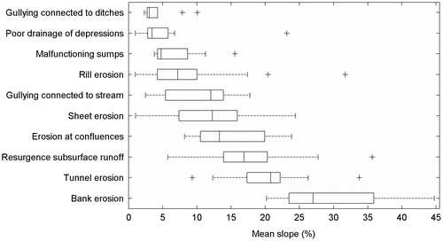
Bank erosion occurred on the steepest slopes, with a mean of 30% (n = 7, SD = 8%, min = 20% and max = 45%), followed by tunnel erosion, which was observed on 9% slopy terrain before ending in river banks of 34% slope (mean = 21%, n = 16, SD = 6%). Resurgence of subsurface runoff or unconfined groundwater occurred on slopes of 6% to 36% (mean = 17%, n = 26, SD = 7%).

Erosion at confluences took place on mean slopes of 15% (n = 16, and SD = 5%). Sheet erosion occurred on slopes 1–24% (mean = 12%, n = 99, SD = 6%). Ephemeral field gullying connected to stream was observed on slopes averaging 11% (n = 38), while rill erosion occurred on average slopes of 8% (n = 83).

Based on these observations, seven erosion categories were very active on sloping lands where erosion control would not have been easy (slopes > 8%), thus resulting in intensive erosion processes. The three remaining erosion categories – erosion due to malfunctioning drainage sumps, poor drainage of depressions and ephemeral field gullying connected to ditches – were observed on slopes ranging from 2–8%. From Figure 7, three is a direct link between erosion category and slope type, where some categories are explicitly found on certain slopes, such as bank erosion with slopes between 20 and 45%, and erosion at confluences originating on slopes of 8–24%, in line with the theoretical description of erosion types (AAFC and MAPAQ 2007).

In addition, when the erosion features were located on slopes greater than 8% next to watercourses, they were found to be hydrologically and sedimentologically connected to watercourses (namely tunnel erosion, bank erosion, erosion at confluences and ephemeral field gullying connected to streams). On flat landscapes (slopes < 8%), such hydrological and sedimentological connections were not observed (Figure 7).

The different erosion categories and their occurrences (total length) on different soil types are presented in Table 5. There are more erosion features in the soil series Chaloupe (Ce), with a total length of 2279 m (28% of all erosion). However, this soil type was found in three zones, which explains the high occurrence of erosion observations (n = 88, total area = 22.9 ha). Soils with good drainage (e.g., Brunisols) were equally affected by erosion compared to soils with imperfect drainage (Podzols), while many of the aforementioned erosion features were observed on Gleysols.

Table 5. Erosion categories and soil type.

Soil				Total length of erosion features surveyed in each category 1 to 10, l (m)										Total length L (m) and n^p
order	Series^z (zone^y)	Texture	Drainage	1	2	3	4	5	6	7	8	9	10
Brunisols	Fa (1)	Coarse loamy	Good	352								124	40	516 n = 10
	Ba (2)			64	351			18				92		525 n = 25
	Pc (7,8)	Loam		292	164	215	17	15		44	355	630		1,732 n = 54
Gleysols	Ce (4, 5, 10)	Coarse loamy	Imperfect	528	603	161		377	193		133	205	79	2,279 n = 88
	Ri-e (6,9, 11,12)	Clay	Moderately good	437	231	24		28	208	11		587		1,526 n = 77
Podzols	J (1)	Sandy	Imperfect	75	169	7						288	245	784 n = 27
	Ac (3)			84	8	47	50	350	107	106		57	35	844 n = 45

Series^z: Fa, Farmington; Ba, Batiscan; Pc, Pontiac; Ce, Chaloupe; Ri-e, Rideau; J, Saint-Jude; Ac, Achigan. (zone^y): zone 1 to 12 surveyed. n^p = number of features observed. An empty cell indicates that this erosion category was not found on this particular soil.

The main finding from the survey is that erosion features are highly correlated with the rate of change of slope. As such, there is a topographical control on hydrological connectivity – that drives sediment from uphill cultivated lands affected by erosion to the watercourse. This sediment connectivity occurred even though riparian buffer strips of 1 to 3 m were in the landscape as required by the policy Protection of riverbanks, littoral zones and floodplains of the MDDEP (2007a) – and this regardless of their ability to conserve soil and water.

To reduce sediment connectivity and erosion rates on steep cultivated hillslopes, new conservation measures need to be adopted. For this, many erosion control measures described by AAFC and MAPAQ (2007) can be leveraged – and used in conjunction with an extended riparian buffer strip that takes advantage of the topographical control on sediment connectivity to better conserve soil and water.

Observed erosion processes, proposed conservation measures, and GIS-based determination of suitable riparian buffer widths

Ephemeral field gullying connected to stream was the category most observed in the field, with 38 features totaling 1983 m. Slopes range from 2–18%, with a mean of 11% (SD = 4%). In this category, the sedimentological connectivity began uphill on flat agricultural land and ended in the riparian buffer strip and the stream. In some instances, while approaching the buffer strip, the high-velocity flowing water in the gullies was capable of excavating tunnels and water reached the stream by passing underground – that is, under the narrow 1–3 m vegetative strip.

On flat cultivated parcels with ∼2% slopes, superficial and isolated sheet and rill erosion processes were active due to rainfall erosivity. However, because of the connectivity induced by steep slopes where ephemeral gullies occurred, these uplands exported fertile soils and associated pollutants. The sedimentological connectivity was thus established by the ephemeral steep gullies which were in turn responsible for the transport of the sediments and pollutants to the stream.

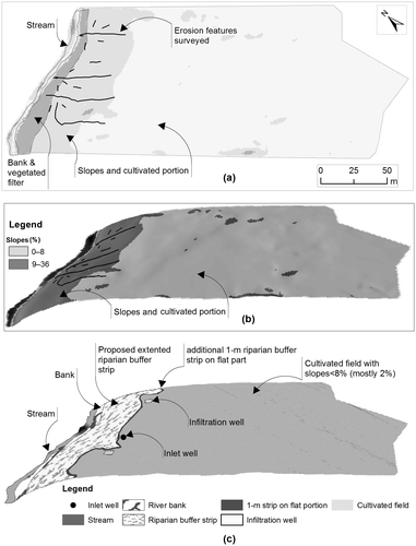
In comparison to the size of an agricultural parcel, steep cultivated slopes constituted only a very small percentage of the total area. As such, a possible solution to the observed erosion processes could be to simply stop cultivating these steep slopes, and convert them into vegetative areas instead, that is, designate them as conservation areas. To illustrate this idea, consider for example the agricultural parcel comprising zone 12, as shown in Figure 8a. The parcel has an area of 7.1 ha and is located between two river banks. Erosion features were surveyed close to the left river bank. The area of the portion of the parcel draining to the left is 2.5 ha (Figure 8a). The direction of water flow on the parcel was determined from a 1-m DTM, along with hydrological tools that simulate surface water flow, accumulation and runoff (ESRI 2012). A closer view of the parcel draining to the left where features of ephemeral gullies connected to stream were surveyed is given in Figure 8b. The active processes of ephemeral gullies on steep slopes enhance the erosion, transport and deposition of sediments and associated pollutants from all over the parcel portion into the buffer strip and the stream (a photo of this process is shown in Figure 6, for the illustration of ephemeral field gullying connected to stream). At the same location, two 2.5-m long tunnel erosions (mean length) were observed (tunnel erosion that goes under the buffer strip).

Figure 8 Cultivated slopes, water flow direction and erosion features; (a) cultivated parcel comprising zone 12; (b) closer view of the parcel portion draining towards the erosional zone surveyed.

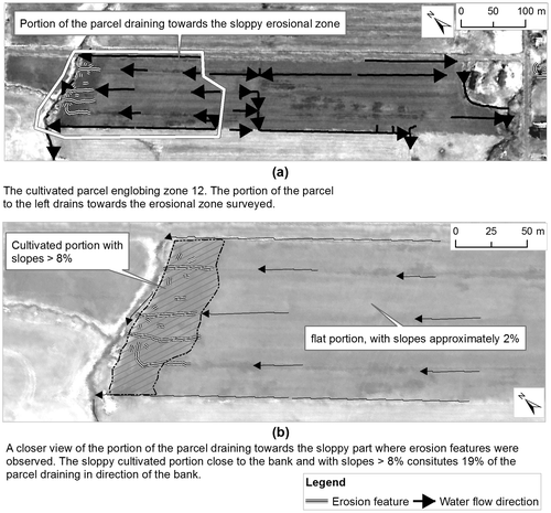
The steep cultivated slopes (> 8%) shown in Figure 8b have an area of 0.47 ha, which is 19% of the total area of the parcel portion draining to the left. If these 19% of steep slopes were no longer cultivated, but converted to vegetated strips (i.e., conservation areas), no more ephemeral gullies connected to stream would be observed. Additionally, the superficial and isolated sheet and rill erosions on the flat portion would no longer have gullies to deliver sediments and associated pollutants to the stream. Consequently, the total erosion from that parcel portion may well decrease by a large amount (possibly more than 19% – the percentage of slopes to be conserved). The steep slopes that are proposed for conservation are about 40–60 m long, and these would be exactly the width of the riparian zone that would need to be implemented.

Figure 9a shows a plan view of the current situation of zone 12, with an equivalent 3D view in Figure 9b (vertical exaggeration of 3). Figure 9b shows the flat cultivated ledge, as well as cultivated steep slopes > 8%, and where erosion features were observed. The proposed action to no longer cultivate these steep slopes near the embankment is illustrated in Figure 9c, which shows the stream, the river bank and the proposed vegetative filters with variable widths of 40–60 m on the steep slopes. Beyond the vegetative strip, an additional buffer strip of 1–2 m is maintained on the plateau, so that flowing water will enter into the extended strip with little momentum. Once past this additional buffer strip, drainage systems could be installed, including inlet and infiltration wells and permeable trenches as means to drain water from the parcel to the stream (AAFC and MAPAQ 2007).

Figure 9 Conservation measures proposed; (a) the current situation in plan view and (b) in three-dimensional (3D) view; (c) the proposed conservation measures in 3D view.

Sheet erosion was the second most observed category in the field, particularly on bare soil on steep terrain. If conservation measures, such as those proposed in Figure 9c, were adopted, sheet erosion on slopes near watercourses would decrease. On the other hand, superficial and isolated sheet erosion on slopes ∼2% will always occur, which could be easily controlled by a good vegetation cover, reduced tillage and balanced rotation (with grassland or green-manure catch crops or intercropping) (AAFC and MAPAQ 2007). Any ensuing sediments would be retained in the inlet and infiltration wells, and the permeable trenches, and thus would no longer have the opportunity to join the stream through gullying.

Rill erosion was the third most observed category in the field, and was observed on both steep hillslopes and flatter areas. Like sheet erosion, the proposed measures to refrain from cultivating steep slopes near river banks would greatly help to reduce rill erosion in such places. On flat terrain, rill erosion could be controlled by forage crops, reduced tillage or direct seeding and cross slope cropping (AAFC and MAPAQ 2007).

Poor drainage of depressions, resulting from improper drainage methods, was the fourth most observed category. Solutions to this problem would be levelling, infiltration and inlet wells or permeable trenches and grassed waterways (AAFC and MAPAQ 2007).

Resurgence of subsurface runoff or unconfined groundwater was the fifth most observed category, mostly on bare soils with slopes > 8% and close to river banks. The proposed action to no longer cultivate these steep slopes would directly resolve this erosion problem on this particular landform.

Erosion due to malfunctioning drainage sumps was the sixth most common category. In fact, the inlet well system is much more efficient than drainage sumps, and should be adopted instead (AAFC and MAPAQ 2007).

Erosion at confluences was the seventh most observed category with occurrences on slopes ranging from 8–24% (mean 15%, SD = 5%). On some occasions, ephemeral gullies changed into erosion at confluences. In such cases, the proposed action to convert steep slopes into vegetated filter would solve the problem. For the other cases, the solutions would involve grassed and rock chutes and drainage ditches (AAFC and MAPAQ 2007).

Ephemeral field gullying connected to ditches was the eighth most observed category. This erosion was more active on flat area with slopes ∼2%. On such slopes, effective conservation measures would be the same as for rill erosion.

Bank erosion was the ninth most observed category with seven features and 127 m total. The slopes range from 20–45%, with a mean of 30% (SD = 8%). In addition to measures to no longer cultivate steep slopes, other solutions would be rock chute and inlet well with berm (AAFC and MAPAQ 2007).

Tunnel erosion was the least observed category with occurrences on slopes ranging from 9–34% (mean 21%, SD = 6%). The tunnels had diameters of 30–70 cm, depths of 20–60 cm and lengths of 3–13 m (mean = 6.4 m, n = 16, and SD = 3 m). Tunnel erosion was observed in steep cultivated hillslopes near the river bank. Therefore, the proposed action to conserve these areas would directly solve the problem.

Discussion

By detailing the conservation measures for each erosion category, it is clear that the proposed action to no longer cultivate steep slopes would directly solve most erosion problems observed in the field, except for drainage depressions, malfunctioning sumps and isolated rill and sheet erosions active on flat areas. These erosion problems, however, have their solutions listed in extension bulletins published by AAFC and MAPAQ (2007).

As confirmed in previous field studies, slope plays an important role in erosion processes, such that steep slopes are definitely prone to erosion (e.g., Jankauskas and Fullen 2002). On such slopes, the easiest way to proceed is to conserve the entire slope up to the flat ledge with an extended riparian buffer strip, thus effectively taking into account the slope gradient and its length (LS), which is the determining parameter for topographic characterization (e.g., Nigel and Rughooputh 2010b).

On flatter slopes < 8%, the method to determine the width of riparian buffer strips should be to use a mathematical model that takes into account not only topography, but also soil type, turbulent flow, etc. Such a model has been recently developed (the Vegetated Filter Dimensioning Model, VFDM) by Gumiere et al. (2013). Other existing physical models and tools to dimension riparian buffers in flat areas can be used, such as the Vegetative Filter Strip Modeling System model of Muñoz-Carpena et al. (1999), the TRAVA model of Deletic (2001) and simpler tools devised for practical applications by Dosskey et al. (2002, 2008) and Bentrup (2008).

The current regulations on riparian buffer strips in Québec (MDDEP 2007a) can now take advantage of the aforementioned findings (concerning specifically the types of landforms and slopes of the 12 erosional zones surveyed in the La Chevrotière watershed). As more studies on the subject are performed and for more diverse watersheds, it will be possible over the years to build up a strong database and rationale to start incorporating these scientific findings into soil and water conservation policy formulation (Lackey 2007; Irvine 2009; Bui et al. 2011).

Locally, from a farmer’s standpoint, it may be argued that the conversion of large sections of slopes into riparian buffer strips will decrease the land available for agricultural productivity, thus resulting in economic losses. However, the current provincial “Prime-Vert” program supports farms so that they can comply with provincial laws, regulations and environmental policies (MAPAQ 2012). In the event that a modified policy requires steep cultivated lands next to watercourses to be converted to conservation areas, then the “Prime-Vert” program would have to accommodate the monetary compensation for such land conservation scenarios – albeit this could be quite complex to implement in Québec, as discussed by L’Italien (2012). In addition to provincial programs, other organisations may also be interested in providing compensation for conservation scenarios. For instance, during the 2006–2010 period, the “Fondation de la Faune du Québec” put together a program of monetary compensation to 522 farmers for land and biodiversity conservation next to watercourses (Fondation de la Faune du Québec [FFQ] 2011).

An extended riparian buffer strip, as proposed in this study, would also be beneficial to biodiversity. For instance, Spackman and Hughes (1995) showed that riparian buffer strip widths of 10–15 m can recover 90% of terrestrial vascular plants found in their territory (Vermont, USA), with birds and mammals establishing well beyond this distance. Based on studies in the Boyer River watershed in Québec, Maisonneuve and Rioux (2001) recommended that to maintain a good biodiversity of small mammals and herpetofauna, there needs to be a complexity of vegetation structure in a riparian buffer strip (woody, shrubby and herbaceous), and that the number of species increases with an increase in riparian buffer width.

Conversion of steep cultivated slopes into buffer strips would also be economically beneficial to farmers through the gains on reduced fertilizers and reduced soil loss – since soil has its own value too, as well as reduced time spent repairing the erosion scars (MDDEP 2007b). Watershed organizations such as CAPSA also have the technical know-how and manpower required to assist farmers in such conservation scenarios and make their actions profitable – both economically and environmentally.

Furthermore, for this study watershed, 34% of the land was used for cultivation, which is well above the recommended 5% by the MDDEP (2010) to sustain limited impact from nutrients runoff, particularly phosphorus. Therefore, the conversion of steep slopes into vegetated strips would be much more beneficial than detrimental to the La Chevrotière watershed.

Conclusions

The digital terrain analysis and field and remote sensing surveys performed in this work enabled demonstrating that the real 3D landscape features – driving sedimentological connectivity from upland erosion to watercourses (by passing through the riparian buffer strip) – are not properly taken into account in the current 2D landform model implemented in the provincial policy that regulates vegetated filters. This omission results in an inadequate protection of watercourses and water bodies against environmental damages due to accelerated erosion processes and resulting water pollution. For instance, the erosion process ephemeral field gullying connected to stream was shown not only to cause soil loss on steep slopes, but also to convey soil particles from uphill flat lands to streams. Supported by 3D terrain illustrations, it is proposed that the riparian buffer should include the distance from the river bank up to the ledge uphill where normal superficial sheet and rill erosion sediments would not have the chance to enter the stream. This way, the vegetated strip would effectively act as a boundary between the watercourse and the damaging uphill erosion processes.

Acknowledgements

This research was supported by the Growing Forward initiative (Cultivons l’avenir), a joint partnership between Agriculture and Agri-Food Canada (AAFC) & the Ministère de l’Agriculture, des Pêcheries et de l’Alimentation du Québec (MAPAQ), under the “Programme de soutien à l’innovation en agroalimentaire” (PSIA), Project # 811083. The authors wish to thank Stéphane Blouin of CAPSA for leading the visit to the erosion zones. The authors also thank Yassin Aljane and Rachid Lhissou for their assistance during the surveys.

References

- Agriculture and Agri-Food Canada (AAFC). 2010. The Canadian system of soil classification, 3rd ed. Agriculture and Agri-Food Canada. http://sis.agr.gc.ca/cansis/taxa/cssc3/intro.html. (accessed August, 2012).
- Agriculture and Agri-Food Canada (AAFC), and Ministère de l’Agriculture, des Pêcheries et de l’Alimentation du Québec (MAPAQ). 2007. Diagnosis and solutions for field erosion and surface drainage problems. http://www4.agr.gc.ca/resources/prod/doc/terr/pdf/Diagnosis_and_Solutions_for_Field_Erosion.pdf. (accessed August, 2012).
- Anderson, N.T., and G.B. Marchisio. 2012. WorldView-2 and the evolution of the DigitalGlobe remote sensing satellite constellation: Introductory paper for the special session on WorldView-2. In Algorithms and Technologies for Multispectral, Hyperspectral, and Ultraspectral Imagery XVIII, 83900L. Proc. SPIE, edited by Sylvia S. Shen and Paul E. Lewis. Baltimore, MD: Spie Digital Library.
- Avery, A., S. Thibaudeau, S. Lamoureux, A. Bélanger, and C. Grondin. 2011. Fiche technique : Des actions pour la faune en milieu agricole – Les habitats des poissons. Fondation de la Faune Québec. http://www.fondationdelafaune.qc.ca/documents/x_guides/968_fiche_poissons.pdf. (accessed September, 2012).
- Bentrup, G. 2008. Conservation buffers: Design guidelines for buffers, corridors, and greenways. Gen. Tech. Rep. SRS-109. Asheville, NC: Department of Agriculture, Forest Service, Southern Research Station.
- Boardman, J. 2006. “Soil erosion science: Reflections on the limitations of current approaches.” CATENA 68(2–3): 73–86.
- Bourque, P.A. 2004. Le Québec géologique. Dans Planète Terre. Département de géologie et de génie géologique de l’Université laval. http://www2.ggl.ulaval.ca/personnel/bourque/intro.pt/planete_terre.html. (accessed August, 2012).
- Bui, E.N., G.J. Hancock, and S.N. Wilkinson. 2011. “Tolerable hillslope soil erosion rates in Australia: Linking science and policy.” Agriculture, Ecosystems & Environment 144(1): 136–149.
- La Corporation d’aménagement et de protection de la rivière Sainte-Anne (CAPSA). 2011. Organisme des bassins versants des rivières Sainte-Anne, Portneuf, La Chevrotière et Belle-Isle). Portrait préliminaire des nouvelles zones de gestion intégrée de l’eau par bassin versant de la CAPSA : les bassins versants des rivières La Chevrotière et Belle-Isle, St-Raymond, Québec. Saint-Raymond, QC: CAPSA.
- Deletic, A. 2001. “Modelling of water and sediment transport over grassed areas.” Journal of Hydrology 248(1–4): 168–182.
- Deslandes, J., and J. Belvisi. 2008. Outils de diagnostic multi-échelle pour des applications en matière de lutte contre l’érosion. Géomatique appliquée à la régie des sols : pour des terres bien égouttées et une eau propre. St-Hyacinthe, 21 janvier 2008. http://www.agrireseau.qc.ca/references/6/Belvisi_JetDeslandes_J.pdf. (accessed August, 2012).
- Dillaha, T.A., R.B. Reneau, S. Mostaghimi, and D. Lee. 1989. “Vegetative filter strips for agricultural nonpoint source pollution control.” Transactions of the American Society of Agricultural Engineers 32(2): 513–519.
- Dosskey, M.G., D.E. Eisenhauer, and M.J. Helmers. 2005. “Establishing conservation buffers using precision information.” Journal of Soil and Water Conservation 60(6): 349–354.
- Dosskey, M.G., M.J. Helmers, and D.E. Eisenhauer. 2008. “A design aid for determining width of filter strips.” Journal of Soil and Water Conservation 63(4): 232–241.
- Dosskey, M.G., M.J. Helmers, D.E. Eisenhauer, T.G. Franti, and K.D. Hoagland. 2002. “Assessment of concentrated flow through riparian buffers.” Journal of Soil and Water Conservation 57(6): 336–343.
- Environment Canada (EC). 2007. Canadian daily climate data (CDCD). Environment Canada, Ottawa, Ontario. ftp://ftp.tor.ec.gc.ca/Pub/Data/Canadian_Daily_Climate_Data_CDCD/. (accessed September, 2012).
- Environment Canada (EC). 2012a. National climate data and information archive. Environment Canada. http://www.climate.weatheroffice.gc.ca/Welcome_f.html. (accessed August, 2012)
- Environment Canada (EC). 2012b. Short-duration rainfall intensity-duration-frequency (IDF). Environment Canada. http://climate.weatheroffice.gc.ca/prods_servs/index_e.html. (accessed January, 2013).
- Environmental System Research Institute (ESRI). 2010. ArcGIS Software Version 10. Redlands, CA: Environmental System Research Institute.
- Environmental System Research Institute (ESRI). 2012. ArcHydro Tools 2.0 for ArcGIS10. Redlands, CA: Environmental System Research Institute.
- Fondation de la Faune du Québec (FFQ). 2011. Wildlife initiatives – Biodiversity in farming communities. Fondation de la Faune du Québec. http://www.fondationdelafaune.qc.ca/initiatives/biodiversite_en_milieu_agricole. (accessed September, 2012).
- Gagnon, É., and G. Gangbazo. 2007. Efficacité des bandes riveraines : analyse de la documentation scientifique et perspectives Développement durable, environnement et parcs Québec (MDDEP). http://www.mddep.gouv.qc.ca/eau/bassinversant/fiches/bandes-riv.pdf. (accessed August, 2012).
- Gordon, R.J., A.C. VanderZaag, P.A. Dekker, R. De Haan, and A. Madani. 2011. “Impact of modified tillage on runoff and nutrient loads from potato fields in prince Edward Island.” Agricultural Water Management 98(12): 1782–1788.
- Gumiere, S.J., Y. Le Bissonnais, D. Raclot, and B. Cheviron. 2011. “Vegetated filter effects on sedimentological connectivity of agricultural catchments in erosion modelling: a review.” Earth Surface Processes and Landforms 36: 3–19.
- Gumiere, S.J., A.N. Rousseau, D.W. Hallema, and P.-É. Isabelle. 2013. “Development of VFDM: A riparian vegetated filter dimensioning model for agricultural watersheds.” Canadian Water Resources Journal 38(3): 169–184.
- Irvine, J.R. 2009. “The successful completion of scientific public policy: Lessons learned while developing Canada’s wild salmon policy.” Environmental Science & Policy 12(2): 140–148.
- Jankauskas, B., and M.A. Fullen. 2002. “A pedological investigation of soil erosion severity on undulating land in Lithuania.” Canadian Journal of Soil Science 82(3): 311–321.
- Knowler, D., and B. Bradshaw. 2007. “Farmers’ adoption of conservation agriculture: a review and synthesis of recent research.” Food Policy 32(1): 25–48.
- Lackey, R.T. 2007. “Science, scientists, and policy advocacy.” Conservation Biology 21(1): 12–17.
- Lal, R. 2001. “Soil degradation by erosion.” Land Degradation & Development 12(6): 519–539.
- L’Italien, F. 2012. L’accaparement des terres et les dispositifs d’intervention sur le foncier agricole – Les enjeux pour l’agriculture québécoise. Research Report. Institut de recherche en économie contemporaine (IREC), Montréal. http://www.upa.qc.ca/ScriptorBD/publication/204694/Accaparement%20des%20terres%20Mars%202012.pdf. (accessed September, 2012).
- Liu, Y., B. Fu, Y. Lü, Z. Wang, and G. Gao. 2012. “Hydrological responses and soil erosion potential of abandoned cropland in the Loess Plateau, China.” Geomorphology 138(1): 404–414.
- Lobb, D.A., S. Li, and B.G. McConkey. 2010. “Soil erosion risk (integrating the risks of wind, water and tillage Erosion): national coverage 1981 to 2006.” In Environmental Sustainability of Canadian Agriculture: Agri-Environmental Indicator Report Series – Report #3, edited by W.M.R. Eilers, L. Graham and A. Lefebvre. Ottawa, ON: Agriculture and Agri-Food Canada.
- Maisonneuve, C., and S. Rioux. 2001. “Importance of riparian habitats for small mammal and herpetofaunal communities in agricultural landscapes of southern Québec.” Agriculture, Ecosystems & Environment 83(1–2): 165–175.
- Michaud, A.R., I. Beaudin, J. Deslandes, F. Bonn, and C.A. Madramootoo. 2007. “SWAT-Predicted influence of different landscape and cropping system alterations on phosphorus mobility within the Pike River watershed of south-western Québec.” Canadian Journal of Soil Science 87(3): 329–344.
- Ministère de l’Agriculture, des Pêcheries et de l’Alimentation du Québec (MAPAQ). 2012. Prime-Vert program to promote and disseminate good agricultural practices. The Ministère de l’Agriculture, des Pêcheries et de l’Alimentation du Québec. http://www.mapaq.gouv.qc.ca/fr/productions/md/programmes/pages/primevert.aspx. (accessed September, 2012).
- Ministère de l’Agriculture, des Pêcheries et de l’Alimentation du Québec (MAPAQ) and Institut de recherche et de développement en agroenvironnement (IRDA). 2003. Pédologie (fichiers numériques) de source inventaire des terres du Canada de Aménagement rural et développement de l’agriculture (ARDA). échelle de numérisation: 1 : 20 000, année de numérisation: 1998–2003. Ville de Québec, Québec: MAPAQ & IRDA.
- Ministère du développement durable de l’environnement et des parcs (MDDEP), 2002. Règlement sur les exploitations agricoles (REA): Développement durable, environnement et parcs Québec. Québec: QC. http://www.mddep.gouv.qc.ca/milieu_agri/agricole/index.htm. (accessed August, 2012).
- Ministère du développement durable de l’environnement et des parcs (MDDEP). 2007a. Protection des rives, du littoral et des plaines inondables : Guide d’interprétation. In Ministère du développement durable de l’environnement et des parcs. Direction des politiques de, l. e., and Québec. Service de l’aménagement des eaux, edited by. C. Michaud, P. Dubois, P., Québec. QC: Développement durable, environnement et parcs Québec.
- Ministère du développement durable de l’environnement et des parcs (MDDEP). 2007b. Vos lacs et cours d’eau – Une valeur à préserver en milieu agricole. Québec, QC: Développement durable, environnement et parcs Québec. http://www.mddep.gouv.qc.ca/eau/rives/agricole/index.htm. (accessed August, 2012).
- Ministère du développement durable de l’environnement et des parcs (MDDEP). 2007c. Vos lacs et cours d’eau – Une richesse collective à préserver. Québec, QC: Développement durable, environnement et parcs Québec. http://www.mddep.gouv.qc.ca/eau/rives/richesse/LacsCoursDeau.pdf. (accessed August, 2012).
- Ministère du développement durable de l’environnement et des parcs (MDDEP). 2010. Les bases scientifiques du Règlement Exploitation Agricole (REA). Québec, QC: Développement durable, environnement et parcs Québec. http://www.mddep.gouv.qc.ca/milieu_agri/agricole/bases.pdf. (accessed August, 2012).
- Ministère du développement durable de l’environnement et des parcs (MDDEP). and Centre d’expertise hydrique du Québec (CEHQ). 2011. Fiche signalétique de la station 050501 – La Chevrotière. Québec, QC: Développement durable, environnement et parcs Québec & Centre d’expertise hydrique du Québec. http://www.cehq.gouv.qc.ca/depot/historique_donnees_som_mensuels/050501_Q_MOY.txt. (accessed September, 2012).
- Ministère du développement durable de l’environnement et des parcs (MDDEP), and Centre d’expertise hydrique du Québec (CEHQ). 2012. Fiche signalétique de la station la Chevrotière. Développement durable, environnement et parcs Québec & Centre d’expertise hydrique du Québec. http://www.cehq.gouv.qc.ca/depot/historique_donnees/fichier/050501_Q.txt. (accessed August, 2012).
- Ministère des Ressources naturelles et de la Faune (MRNF). 2006. Gros Plan Sur La Capitale-Nationale. Structure géologique. Québec City, QC: Ministère des Ressources naturelles et de la Faune.
- Montgomery, D.R. 2007. “Soil erosion and agricultural sustainability.” Proceedings of the National Academy of Sciences of the USA 104(33): 13268–13272.
- Morgan, R.P.C. 2005. Soil Erosion and Conservation. Oxford: Blackwell Publishing.
- Muñoz-Carpena, R., J.E. Parsons, and J.W. Gilliam. 1999. “Modeling hydrology and sediment transport in vegetative filter strips.” Journal of Hydrology 214(1–4): 111–129.
- Nieswand, G.H., R.M. Hordon, T.B. Shelton, B.B. Chavooshian, and S. Blarr. 1990. “Buffer strips to protect water supply reservoirs: a model and recommendations.” Journal of the American Water Resources Association 26(6): 959–966.
- Nigel, R., and S. Rughooputh. 2010a. “Mapping of monthly soil erosion risk of mainland Mauritius and its aggregation with delineated basins.” Geomorphology 114(3): 101–114.
- Nigel, R., and S.D.D.V. Rughooputh. 2010b. “Soil erosion risk mapping with new datasets: an improved identification and prioritisation of high erosion risk areas.” CATENA 82(3): 191–205.
- PCI Geomatics Enterprises. 2011. PCI Focus. Richmond Hill, ON: PCI Geomatics Enterprises.
- Prasuhn, V. 2011. “Soil erosion in the Swiss Midlands: results of a 10-year field survey.” Geomorphology 126(1–2): 32–41.
- Rees, H.W., T.L. Chow, B.J. Zebarth, Z. Xing, P. Toner, J. Lavoie, and J.L. Daigle. 2011. “Effects of supplemental poultry manure applications on soil erosion and runoff water quality from a loam soil under potato production in northwestern New Brunswick.” Canadian Journal of Soil Science 91(4): 595–613.
- Renard, K.G., G.R. Foster, G.A. Weesies, D.K. McCool, and D.C. Yoder. 1997. Predicting Soil Erosion by Water: a Guide to Conservation Planning with the Revised Universal Soil Loss Equation (RUSLE). Tucson, AZ: USDA-ARS, Southwest Watershed Research Center.
- Renschler, C.S., and J. Harbor. 2002. “Soil erosion assessment tools from point to regional scales – the role of Geomorphologists in land management research and implementation.” Geomorphology 47(2–4): 189–209.
- Rousseau, A.N., P. Lafrance, M.-P. Lavigne, S. Savary, B. Konan, R. Quilbé, P. Jiapizian, et al. 2012. “A hydrological modeling framework for defining achievable performance standards for pesticides.” Journal of Environmental Quality 41(1): 52–63.
- Rousseau, A.N., S. Savary, D.W. Hallema, S.J. Gumiere, and E. Foulon. 2013. “Modeling the effects of agricultural BMPs on sediments, nutrients and water quality of the Beaurivage River watershed (Quebec, Canada).” Canadian Water Resources Journal 38(2): 99–120.
- Shi, Z.H., N.F. Fang, F.Z. Wu, L. Wang, B.J. Yue, and G.L. Wu. 2012. “Soil erosion processes and sediment sorting associated with transport mechanisms on steep slopes.” Journal of Hydrology 454–5: 123–130.
- Spackman, S.C., and J.W. Hughes. 1995. “Assessment of minimum stream corridor width for biological conservation: Species richness and distribution along mid-order streams in Vermont, USA.” Biological Conservation 71(3): 325–332.
- Stonehouse, D.P., and M.J. Bohl. 1993. “Selected government policies for encouraging soil conservation on Ontario cash-cropping farms.” Journal of Soil and Water Conservation 48(4): 343–349.
- van Dijk, A.I.J.M., L.A. Bruijnzeel, R.A. Vertessy, and J. Ruijter. 2005. “Runoff and sediment generation on bench-terraced hillsides: Measurements and up-scaling of a field-based model.” Hydrological Processes 19(8): 1667–1685.
- van Dijk, P.M., F.J.P.M. Kwaad, and M. Klapwijk. 1996. “Rentention of water and sediment by grass strips.” Hydrological Processes 10(8): 1069–1080.
- Wall, G.J., D.R. Coote, E.A. Pringle, and I.J. Shelton. 2002. RUSLE-CAN – Universal soil loss equation for application in Canda. Manual for evaluation of soil loss by water erosion in Canada. Contribution No. AAC2244F. Ottawa, ON: Research Branch of Agriculture and Agri-Food Canada (AAFC).
- Wischmeier, W., and D. Smith. 1978. Predicting Rainfall Erosion Losses: a Guide to Conservation Planning. Washington, DC: United States Department of Agriculture.
- Zhu, T.X. 2012. “Gully and tunnel erosion in the Hilly Loess Plateau region, China.” Geomorphology 153–4: 144–155.