Power in the European Union: an evolutionary computing approach

ABSTRACT

Even the best existing model of legislative decisionmaking in the European Union, the compromise model, makes huge prediction errors when it is assumed that each actor’s power is determined by their formal voting weight. A few studies have attempted to improve the model’s predictive accuracy by examining alternative distributions of power, but extending their brute force approach poses daunting computational challenges. In this paper I illustrate how techniques from evolutionary computing can be employed to overcome these challenges. I then demonstrate the new possibilities that this approach opens up by identifying the relative power of each actor that best predicts policy outcomes from the EU-15 period. Some actors appear to punch significantly above or below their formal weight, with power varying dramatically across legislative procedures. My analysis highlights important unanswered questions about power in EU decisionmaking, and potentially indicates fundamental problems with the compromise model or the underlying data.

KEYWORDS:

• Power
• decision making
• evolutionary computing
• bargaining
• European Union

Introduction

If there is one thing that the European Union (EU) does, it legislates. The EU may have no independent military capabilities and a tiny central budget, but each year it adopts hundreds of new laws. This massive corpus of rules creates an internal market amongst the (currently) 27 Member States, regulates the characteristics of traded goods and services, sets agricultural subsidies, establishes common environmental standards, governs food safety and other risks, manages external trade with the rest of the world and much else.

That the EU does so much that is clearly not trivial raises questions about the relative power of each actor in EU legislative decisionmaking, and who is best able to achieve their desired policy outcomes. Yet answers to these questions remain elusive. On the face of it, one might suspect that actors with the most formal voting power in the Council of Ministers, like France and Germany, dominate the legislative process, but the empirical evidence undeniably suggests that they dont. Numerous regression studies have found that states with more votes in the Council do no better, or do consistently worse than states with fewer votes at attaining outcomes nearer their own policy preference. Even the best available model – the compromise model – makes huge errors in predicting policy outcomes when it is assumed that the power of each actor is determined solely by their formal voting weight (Shapley-Shubik Index values).

Which begs the question: what if the compromise model is basically correct but SSI values are problematic? Can we retain the compromise model, given that it is the best to date, but identify power scores that improve the model’s predictions and align them more closely with the regression results? A few studies have attempted to improve the predictive accuracy of the compromise model by investigating sets of alternative power scores for the Commission, Parliament and Member States, but these efforts only scratch the surface, and extending their ‘brute force’ approach more widely poses daunting computational challenges.

The main purpose of this paper is to illustrate how techniques from evolutionary computing can be employed to overcome these challenges. Then, to demonstrate the new possibilities that this approach opens up, I determine how much better we can do in our predictions depending on how far we are willing to allow actor power to deviate from formal voting weight. With the compromise model as the basic building block of my analysis, I employ evolutionary computing to identify the relative power of each actor that best predicts 162 actual policy outcomes in the EU-15, before the 2004 enlargement. The results, whether from a fully optimised model or one that only allows deviations that are much smaller than those considered in previous studies, challenge core assumptions about how the EU operates. Some actors punch significantly above or below their formal weight, with power varying dramatically across legislative procedures.

My analysis proceeds as follows. Section one reviews three well-known items from EU studies that will feature throughout the paper: formal voting power, the Decisionmaking in the European Union (DEU) data, and the compromise model. Section two highlights the mismatch between formal voting power and what we know about EU legislative outcomes, discusses the few previous attempts to explore the accuracy of the compromise model when fit with alternatives to SSI values, and shows that extending the approach of these studies more widely presents an insurmountable computational challenge. Section three introduces an evolutionary computing approach that can overcome this challenge, then applies it to the EU-15 data. Section four discusses the results, identifies unanswered questions, and highlights potential avenues for future research.

Building blocks

In order to critique the use of formal voting power as a predictor of EU legislative outcomes, some preliminary comments about conceptual terminology are required. The literature on EU decisionmaking tends to use the terms ‘power’, ‘power resources’, ‘actual power’, ‘capabilities’, and ‘influence’ interchangeably.¹ Instead of attempting to parse these various terms, I will treat an actor’s power, whether a Member State or the European Commission or the European Parliament, as their ability to secure their preferred legislative outcomes despite initial resistance (Tallberg 2008, 687; Bailer 2004, 101; Thomson and Hosli 2006, 394; Schneider, Finke, and Bailer 2010, 86). Actors will always encounter at least some resistance; given the diversity of preferences on each legislative issue, they are never pushing on an open door.

My distinction between ‘formal’ and ‘informal’ power also follows the terminology commonly used in leading EU studies (Widgrén and Pajala 2006, 239; Thomson and Hosli 2006, although Bailer (2004, 2006) prefers the labels ‘exogenous’ and ‘endogenous’), whereby formal refers to power conferred by the voting weights, agenda setting and veto rules contained in the treaty, and informal denotes any other source of power. The EU’s formal rules can seem labyrinthine, but fortunately only a few key provisions pertain to the present analysis of the period before the 2004 enlargement.² The Commission is the only actor that can formally issue or withdraw a proposal. Formally the Council decides by either unanimity, with one vote per Member State so all must agree in order to pass a law, or qualified majority (QMV), with each state casting a number of votes roughly proportional to its population and about five-sevenths of the total votes is required to adopt a law. Under the consultation procedure, the European Parliament can offer its opinion on a legislative proposal but the Council can ignore it, whereas under the codecision procedure legislative adoption requires the joint agreement of the Parliament and Council.

Those who advocate a voting power approach to understand EU decisionmaking assume that each Member State’s power corresponds with the number of formal votes it has in the Council (Hosli 1996). The first building block of my analysis is therefore the widely used SSI voting power index, which attributes each actor with a score that reflects the proportion of all possible coalitions where they are pivotal; that is, they can cast the decisive vote to turn a losing coalition into a winning one (Shapley and Shubik 1954).³ For relative Member State power, the formal voting rule – QMV or unanimity – matters much more than the European Parliament’s involvement via either consultation or codecision. Under unanimous voting, all states have equal SSI scores since they are all pivotal. Under QMV, large states have more votes than small ones, but, as with most other federal systems, small states are heavily overrepresented. Large states each consistently have two or three times more power than small ones, and power does not differ significantly between the large or between the small states.

One can also calculate SSI scores for the Council, Commission and European Parliament. Under codecision, the Commission has no formal power relative to the Council because, legally, it can be excluded from winning coalitions. The same applies to the Parliament under consultation. Under codecision and QMV, the Parliament is nearly half as strong as the Council, or put another way, about as powerful as France, Germany, Italy and the UK combined. Under consultation and QMV, the Commission has approximately one-third the formal power of the Council. Finally, in the rare situation of codecision and unanimity, the Parliament has one-fifteenth the power of the Council, exactly the same as any individual Member State.

The famous European Union Decisionmaking dataset, from the book The European Union Decides (Thomson et al. 2006), provides the second building block of my analysis. This is the only available dataset that contains information on policy outcomes across many cases, which is necessary to systematically investigate relative power in the EU. A team of researchers gathered data during the EU-15 period on 162 controversial policy issues contained in 66 legislative proposals from the Commission. For each issue they were able to identify and scale the policy alternative most preferred by each actor (the fifteen Member States, the Commission and EP), the salience each actor attached to the issue, and the position of the eventual legislative outcome. This initial dataset was later expanded to include 125 proposals, half of them from the post-2004 period (for details on the DEUII dataset see Thomson et al. 2012). It is essential to note that in using the DEU dataset I accept the project’s simplification of the EU’s complex multi-level environment. Although each actor’s preferred position is likely shaped by a combination of personal views, partisan considerations, ideological concerns and both domestic and supranational lobbying efforts, the dataset does not attempt to trace the coded ideal points back to some set of proximate causes or microfoundations.

The third building block in my analysis is the so-called ‘compromise model’. Formalised by Van den Bos (1991) and also used in Bueno de Mesquita and Stokman (1994), the compromise model is similar to a Nash bargaining solution and predicts political outcomes to occur at the weighted mean of actors’ most preferred points, with weights given by the product of power and salience. With n actors,

(1) $O_a=\frac{\sum _{i=1}^n{x}_{ia}{p}_i{s}_{ia}}{\sum _{i=1}^n{p}_i{s}_{ia}}$(1)

where O_a is the predicted outcome on issue a, x_ia is the ideal outcome for actor i on issue a, p_i is the power of actor i, and s_ia is the salience actor i attaches to issue a. Simply put, the model posits that more powerful actors and more intense actors have more influence than the weak or the apathetic (Achen 2006a, 92). Importantly, the model is ‘not concerned with the composition of actors’ power’ (Thomson and Hosli 2006, 402) – power derives from an unspecified combination of formal and informal resources. In the EU context, the only actors are the Member States, Commission, and European Parliament, each of which is treated as a unitary actor. Again, this is a simplification that relegates the messy reality of internal divisions, lobbying and multi-level decisionmaking to the background. Other noteworthy features of the compromise model, to which I return later, are that actors incur no penalty for taking extreme positions, and receive no bonus (or penalty) for how often they take no position, or when holding the Council Presidency.

Previous efforts to improve predictions

The primary conclusion from The European Union Decides was that the compromise model fit with SSI power scores makes the best predictions. Still, this set-up makes large errors. In substantive terms, its predictions typically miss the mark by 17–27 points on a 100 point scale depending on the voting rule and parliamentary procedure involved (Achen 2006b, 276). If Achen is right that ‘a fair test of a model is that it does better than very simple [atheoretical] baselines’ (2006b, 270), then the compromise model as specified in the book is a failure. One obtains just as accurate predictions by ignoring everything else and simply taking the atheoretical mean of the actors’ positions (Achen 2006b, 277). This suggests that something is fundamentally wrong with the nature of the compromise model, or with the DEU data, or with the assumption that SSI scores are a good guide to which actors achieve their preferred legislative outcomes.

Although studies using the DEU data have found that the compromise model significantly outperforms more elaborate procedural models as well as other bargaining models (Achen 2006b, 277; Thomson 2011),⁴ this doesn’t rule out the possibility that the compromise model is merely the best of a weak bunch. As for the DEU data, questions remain about potential measurement error (Slapin 2014; Leinaweaver and Thomson 2014) and the improvements scholars might make particularly through systematic use of newspaper articles (Selck, Yardimci, and Kathan 2009).

Yet what arguably makes the SSI assumption the weakest link is the striking mismatch between formal voting power and what we know about EU legislative outcomes. In every study that has regressed formal voting power (or its equivalent, state population) against bargaining success, formal voting power tests out as insignificant or even negative: states with more votes in the Council (thus higher SSI scores) do no better than, or do consistently worse than states with fewer votes at attaining outcomes nearer their own policy preference (Bailer 2004; Selck and Kuipers 2005; Arregui and Thomson 2009; Aksoy 2010; Thomson 2011; Golub 2012a; Cross 2012; Arregui 2016).⁵ In pairwise comparisons of bargaining success, no large state achieves significantly more than any small state. Moreover, Denmark beats France, Finland beats France and Germany and Italy, Ireland beats France (and perhaps Italy), and Sweden beats France and Italy (and perhaps Germany) (Golub 2012a, 1302–3).

It is reasonable to suspect, therefore, that informal power almost certainly plays a considerable role in EU legislative decisionmaking, especially in bolstering the influence of small Member States, and that considering deviations from SSI values should improve our ability to predict outcomes. But so far we know very little about the distribution of this power. Bailer interviewed experts to compile a measure of each Member State’s informal, endogenous power, conceptualised as their respective negotiating skill and level of information, but these tested out as insignificant when regressed against bargaining success (Bailer 2004; Golub 2012a, 1306). Panke’s measure of each Member State’s ‘range of negotiating activities’ (2011) proved significant when regressed against pooled data on national bargaining success, but not for proposals subject to QMV which are by far the most common (Golub 2012a, 1308). While suggestive, these regression studies are limited in that their findings are divorced from an underlying model of the bargaining process that could have produced them.

My analysis builds on the few previous studies that have tested the compromise model (or the very similar Nash Bargaining Model) with non-SSI power scores. Thomson and Hosli (2006) use the DEU data and treat the relative power of each Member State as entirely formal, given by their SSI score (rescaled so that they sum to 100), but then estimate the informal power of the Commission and EP relative to the Council under different procedures. They do this by brute force, repeatedly fitting the compromise model with different power scores for the EP and Commission in increments of five from 0 to 200. From the 1,681 (41 x 41) combinations of power scores, for each type of legislative procedure they identify the one that provides the most accurate forecasts of actual legislative outcomes. They find, ultimately, that predictions improve significantly if we assume the Commission has less power and the EP has more power under both QMV/CNS and QMV/COD than indicated by their respective SSI scores.⁶ When he reduced the increments between 0 and 200 to one and examined 40,401 combinations (201 x 201), Thomson reached the same conclusions (2011:chapters 8–10).

In two other attempts to investigate informal power within the Council, Thomson uses these estimated non-SSI power scores for the EP and Commission and then alters the power of each Member State (2008, 2011 chapter 9). He fits five variants of the compromise model, one where each Member State is assigned their formal SSI power, and four that allow dramatic deviations from SSI values. In these four competing variants, either all actors have equal power, the five or six largest Member States have equal power and all other states have none, the three largest Member States have equal power and all others have none, or France and Germany have equal power and all others have none. In several situations at least one of these alternative models returns slightly lower average errors than those produced by SSI scores.

Finally, Golub (2012b) attempted to improve upon a compromise model fit with SSI values by investigating whether Member States sell their votes within the Council. For each voting rule and legislative procedure, he tested compromise models with Member States’ power inflated or deflated according to their average net EU budgetary transfers, but none beat the predictions using unadjusted SSI scores.

These few attempts to investigate the predictive accuracy of the compromise model using alternative power scores merely scratch the surface of possibilities. Thomson and Hosli (2006) motivate their analysis by noting that the experts interviewed for the European Union Decides project gave dramatically different estimates of the Council, Commission, and European Parliament’s relative power. They then explored ‘all logical possible combinations of power scores’ (2006, 408) for the Council, Commission and European Parliament, even if these combinations were far outside the range of expert estimates for these three institutions, shown in Table 1.

Table 1. Expert estimates of inter-institutional relative power

Institution	Procedure	Range
Council	COD CNS	62.50–100 71.43–100
Commission	COD CNS	22.22–100 10–100
European Parliament	COD CNS	44.44–100 0–75

Note: The practitioners survey asked 18 informants to rank each institution’s relative power on a scale of zero to one hundred. Data from Thomson (2002). CNS = consultation, COD = codecision.

But the experts also gave dramatically diverse estimates of each Member State’s relative power, as shown in Table 2.

Table 2. Expert estimates of member state relative power

Member State	Range
Austria	0–80
Belgium	25–60
Denmark	10–60
Finland	20–55
France	45–100
Germany	45–100
Greece	10–45
Ireland	10–80
Italy	30–90
Luxembourg	0–95
Netherlands	35–65
Portugal	20–50
Spain	40–100
Sweden	30–55
UK	80–100

Note: Data from Bailer (2004). The practitioners survey asked fifteen informants to rank each Member State’s power on a scale of zero to one hundred.

The enormous range is likely due to the fact that respondents had different professional backgrounds, that they were not requested to distinguish between legislative procedures or policy areas, and that in the DEU data a different policy sector is predominant in each procedure. CNS/QMV proposals overwhelming pertain to agriculture, CNS/UNAN proposals are mostly about Justice and Home Affairs, never about agriculture or the internal market, COD/QMV proposals relate mainly to the internal market, and COD/UNAN proposals deal almost exclusively with the internal market. Thus one expert’s rankings might reflect their views of relative power across all procedures, while another’s might reflect their impression of relative power in the particular sector they are most familiar with, or in situations where QMV rather than unanimity, or codecision rather than consultation applied.

What we really want to know, is how much our predictions improve if we retain the compromise model and relax the SSI assumption for all seventeen actors. This presents an insurmountable computational challenge for the brute force approach taken by Thomson and Hosli. With n actors and p different power scores we would need to determine which of p^n possible solutions produced the most accurate predictions. With fifteen Member States, the EP and Commission, and assuming 41 steps of power as Thomson and Hosli do, this produces 41^17 variants (10^27.4), of which only 1,685 have been compared to date. To try each solution sequentially, as Thomson and Hosli did, would take even the fastest supercomputer, operating at 10^15 calculations per second (1 petaflop), nearly one hundred thousand (10^5) years. Ranking each actor on a more precise 0–100 integer scale increases the number of potential solutions to 101^17 and the required computation time to over 100 billion years (10^11.5). To do so in the enlarged EU with 27 Member States would require 10^31.6 years. Allowing power scores to take on fractional and not just integer values increases the required computing time still further. When all of this was pointed out to me, it provided my colleagues in computer science a certain amount of amusement.

An evolutionary computing approach

Fortunately, an evolutionary computing approach overcomes this computational challenge and allows us to identify the distribution of power that best predicts outcomes. In brief, evolutionary computing works by mimicking the process of natural evolution to find an optimal solution to a given problem. What counts as optimal could involve either minimization or maximization. Perhaps most famous is the travelling salesperson example where a genetic algorithm is used to find the shortest possible travel route between a list of cities while visiting each city only once (Larrañaga et al. 1999). Evolutionary computing is routinely used in situations of complex production processes or choice environments to identify the combination of inputs or particular strategy that will maximize profit. An application of the approach that most readers might have already encountered (or at least benefited from) is in the scheduling of university classes to reduce the number of clashes. The approach explores how the fitness of individuals in a population evolves over subsequent generations through genetic mutation and mating with other individuals within the population (Eiben and Smith 2003). It has been used occasionally in political science, for example to study social norms and cooperation (Axelrod 1986; Hammond and Axelrod 2006), as well as political redistricting and gerrymandering (Liu, Cho, and Wang 2016).

To illustrate how evolutionary computing works, imagine that a company manufactures eight different products, and that the relationship between production levels of each product and the company’s total greenhouse gas emissions is enormously complex. The firm’s objective is to minimize this total, subject to the constraints of remaining profitable and also producing a maximum of 100 units of each product. Altogether, there are 101^8 potential combinations to choose from. Figure 1 translates this ‘real world’ optimization problem into an evolutionary computing problem-solving space. The process begins with a starting ‘population’ of possible solutions, or ‘individuals’, each of which has eight genes, labelled P1, P2, P3 etc. These genes represent the quantity of the eight different products being manufactured. P1 might be televisions, P2 might be refrigerators and so forth. Each individual’s combination of genes (i.e. products) results in a different total amount of greenhouse gas emissions being produced. Fitter individuals have lower emissions. The starting population would normally contain any 100 of the possible individual genetic combinations, but here we have just four in order to simplify the example.

Figure 1. Evolution with one-point crossover.

The evolutionary process proceeds as follows. First, the least fit combination(s) (those with the highest emissions) drop out of the population, then the fittest combinations serve as parents and ‘mate’ with less fit combinations by exchanging some genes with them. The offspring of these matings, plus the survival of the fittest individuals from the first generation, constitute the second generation population. The mating process also allows for mutation, whereby a certain percentage of the genes passed on to offspring deviate from those of the parents. It is a well known evolutionary fact that some offspring can have lower fitness than their parents. Nevertheless, with a large starting population, selection at the mating pool stage tends to weed out inferior individuals and raise the average fitness of the next generation.

In our industrial production example, in the first generation the fourth individual is the fittest because their combination of genes produces the lowest total emissions, which is 4454.8. The mating pool for the second generation, shown on the left-hand side of the middle panel, excludes the least fit individual from the first generation. The fittest individual mates with the second and third fittest individuals, each pairing producing two offspring whose genetic composition is determined by the crossover point, the location in the parental sequences where genes are swapped. Thus with a crossover point of two, the second offspring from the first pairing inherits the first two genes of one parent (75, 74), and the last six genes of its other parent (63, 90, 27, 16, 91, 38). Notice that the first offspring from the first pairing contains a mutation in its eight gene, highlighted in grey. Even though two individuals in the second generation are less fit than their parents, the average fitness of the population improved by over 40 points, as indicated by the lower average emissions. To find the combination of genes that yields the lowest total emissions, we continue this evolutionary process until all members of the population come to resemble the fittest individual in the previous generation, and no further improvement to population fitness is possible through mating or mutation.

When devising a genetic algorithm, the analyst controls several important factors. They can set the size of the mating population (usually 100–200) as well as the mutation rate (usually 1%). Higher values on either will ultimately produce a more optimal solution but will require more time to reach convergence. Crucially, one can also set constraints that all candidate solutions must satisfy, for example that the values of some or all of an individual’s genes must be different from each other, or must fall within a particular range, in our example less than 100. Run as an add-on to Microsoft Excel called ‘Solver’, a standard computer can evaluate thousands of generations in a matter of seconds, and normally converges on the fittest solution within a few minutes or at most an hour. The great advantage of an evolutionary approach over alternatives such as a non-linear gradient reduction algorithm is that on a non-smooth, highly irregular surface the latter tend to get stuck at local minimums and miss the superior, global minimum. And unlike traditional, calculus-based optimization methods, genetic algorithms work even when the search space is noisy and derivatives do not even exist.

To apply the evolutionary computing approach to the EU decisionmaking context, I treat each actor’s power score as a gene, and each possible combination of power scores as an individual with 17 genes. The starting population contains 100 of the possible individual genetic combinations. Each of these individual combinations is plugged into the compromise model (equation 1(1) $O_a=\frac{\sum _{i=1}^n{x}_{ia}{p}_i{s}_{ia}}{\sum _{i=1}^n{p}_i{s}_{ia}}$(1) above) along with the usual data on actors’ ideal outcomes and salience. Each combination produces a prediction error for each DEU issue, and the size of the overall average error across the set of 162 DEU issues reflects that combination’s fitness.

The optimization objective is to find the combination of power scores that minimizes the average error. As many previous studies have done, I examine various subsets of the DEU data, dividing it according to which formal procedure applied – QMV or unanimity in the Council, consultation or codecision by the European Parliament. For each subset of DEU data, I first fit a compromise model with SSI power scores and treat the resulting error rate as the baseline. I then proceed to relax the SSI assumption for all 17 actors.

This involves a crucial decision: how large can deviations from SSI values be while remaining plausible? As a guide, I turned to the previously discussed handful of studies that have investigated deviations from SSI scores, since clearly the authors (and reviewers) considered these deviations reasonable. Thomson and Hosli (2006) examine all logical combinations, and thus deviations for the Commission and European Parliament range up to 125 points above and 44 points below the extremes of the ranges provided by experts. In Thomson (2008, 2011 chapter 9), his ‘big 5/6’, ‘big 3’ and ‘Franco-German’ power distributions assign some Member States power scores that are up to 80 points outside the range of expert assessments.

To find the absolute optimums, I allow the power of each actor to take on any value from 0–100. Investigating such a large search space follows the same logic as examining all logical combinations. Because some might question the face validity of this approach – is it really plausible that several Member States, especially the larger ones, could have power scores of zero? – I also reran the analyses while constraining the power of each actor to fall within the ranges reported by the experts. By comparing the three sets of power scores, for each subset of data we can determine whether, and by how much, we can beat predictions based on formal SSI values depending on how far we are willing to allow actor power to deviate from formal voting weight. To cope with the complexity of the solution space and the possibility of numerous local minimums, I repeated all searches several times with different starting populations.

Discussion

Table 3 presents the results of the evolutionary analyses. These results clearly confirm my main claim: that an evolutionary computing approach allows us to identify power scores for the Commission, Parliament and each Member State that sharply reduce prediction errors from the compromise model. For CNS/QMV proposals, compared to the SSI baseline the optimum model reduces the average error by 12%, whereas the experts range model reduces it by 6%. For CNS/UNAN proposals, the optimal power scores produce a 38% reduction in average error, and the experts range model produces a 12% reduction. For COD/QMV proposals, the optimum delivers a 29% reduction in average error and the experts range model yields a 16% reduction. There are very few proposals subject to codecision and unanimity. Inferences about this procedure are therefore particularly tenuous, given the outsized impact that reducing the prediction error for a single issue has on the average, as well as the possibility that the estimated power score for a given actor reflects the fact they strongly opposed or supported the handful of particular issues that just happened to be processed under these procedures. With these caveats in mind, the optimum produces a dramatic 68% reduction in average error, whereas the more constrained experts range model offers a 38% reduction.

Table 3. Prediction errors using formal and estimated power scores

	COM	EP	AUS	BEL	DK	FIN	FR	GER	GRE	IRE	IT	LUX	NL	POR	SP	SW	UK	Avg. Error
CNS/QMV (55)
SSI	100	0	14.20	16.89	11.46	11.46	34.36	34.36	16.89	11.46	34.36	7.37	16.89	16.89	28.40	14.20	34.36	23.3
Experts range	100	61.42	36.77	11.49	4.60	25.28	20.69	45.97	20.69	4.60	13.79	0	16.09	21.4	45.97	25.28	36.77	21.9
Optimum	100	70.39	33.18	0	0	35.06	0	29.61	57.03	0	0	0	0	0	52.91	65.89	6.14	20.5
CNS/UNAN (39)
SSI	0	0	100	100	100	100	100	100	100	100	100	100	100	100	100	100	100	17.3
Experts range	40	0	0	25	60	20	100	100	45	80	90	0	35	20	40	55	100	15.3
Optimum	0	0	0	0.06	100	0	54.47	0.001	0	0	35.78	0	0	0	0	7.51	18.19	10.8
COD/QMV (56)
SSI	0	100	10	12.14	7.81	7.81	26.10	26.10	12.14	7.81	26.10	4.55	12.14	12.14	21.34	10	26.10	27.3
Experts range	50	100	0	14.20	34.09	31.25	25.57	32.21	5.68	45.45	17.05	0	36.93	11.36	22.73	31.25	56.82	22.9
Optimum	9.78	29.35	0	0	0	82.61	0	0	4.35	94.57	0	40.22	10.87	0	15.22	100	0	19.4
COD/UNAN (12)
SSI	0	100	100	100	100	100	100	100	100	100	100	100	100	100	100	100	100	19.2
Experts range	26.31	100	0	7.47	17.94	16.44	13.45	13.45	13.45	23.92	8.97	28.40	10.46	14.95	11.96	8.97	29.90	12.0
Optimum	0.19	40.09	0	0.01	0	0	18.08	0	28.81	100	0.03	0.05	0	2.06	14.02	0.01	3.88	6.1

Note: Cell entries are power scores entered into the compromise model for each actor. For the SSI models, scores are ‘variant two’ Shapley Shubik Index values, normalised so that the strongest actor scores 100. For the other models, scores are from an evolutionary algorithm constrained so that each actor’s power can be any value from 0 to 100 (optimum) or any value within the range assessed by experts. QMV = qualified majority voting, UNAN = unanimous voting, CNS = consultation, COD = codecision.

That the estimated scores often bear no relation to SSI values suggests that while it is ‘naïve’ (Hayes-Renshaw and Wallace 2006, 252) to assume that all Member States carry equal weight in the Council, it is just as naïve to presume that their true power is reflected in their formal voting weights. But beyond this, what the estimates tell us about how the EU operates depends on the plausibility of the imposed constraints, and even then the analysis highlights important unanswered questions.

If we follow the approach taken by Thomson and Hosli (2006), whereby all logical combinations of power are deemed plausible, my optimal models suggest that EU legislative outcomes pre-2004 were determined almost entirely by a different group of between three and eight of the 17 actors, depending on the procedure involved, and that within these groups some small Member States, especially Sweden, Ireland, Finland and Greece, tended to punch far above their weight while large Member States tended to punch far below theirs. Equally striking, however, is that group membership as well as ranking within each group is often so different across procedures. For example, Austria and Germany both appear highly and equally influential for CNS/QMV proposals yet powerless under all other procedures. Sweden is extremely powerful for proposals subject to QMV but virtually powerless for those subject to unanimity, while Ireland dominates negotiations subject to codecision but is powerless under consultation. And the Big 4 are each entirely powerless under COD/QMV.

Constraining each actor’s power to fall within the range identified by experts is arguably far more plausible. Results from these models suggest that legislative outcomes depend on groups of between 12 and 14 actors, and that under most procedures several small states have as much or more power than Germany, France, the UK and especially Italy. In some ways, fitting the compromise model with these estimated power scores brings its predictions more in line with the aforementioned regression findings and head-to-head comparisons of bargaining success in which large states did no better or indeed did worse than small states. But even in the more constrained models it is surprising how dramatically the estimated relative power of most actors varies across procedures.

What are the estimated scores picking up that would explain these surprising patterns? I suspected that three factors which don’t feature in the compromise model might provide answers: each actor’s spatial extremity, the proportion of issues on which each actor takes a position, and which state holds the Council Presidency (Bailer 2004; Arregui and Thomson 2009; Thomson 2011; Golub 2012a). Actors who stake out extreme positions risk marginalizing themselves, decreasing their coalition potential and thus their influence on legislative outcomes. Actors who take fewer positions and focus their energy on a narrower range of issues tend to carry more weight and achieve greater bargaining success. And decision outcomes tend to be closer to the preferences of whichever state holds the Presidency than to the preferences of other actors.

My initial investigation of these factors suggests two things. First, that based on their expected effects, none of them account well for the estimated power scores. For each procedure, the most powerful actors are not the ones who took the fewest positions, or the fewest extreme positions, or who held the Presidency most often when the final decisions were reached. And none of the factors appear related to estimated relative power under unanimous voting. Second, that for proposals subject to QMV, spatial extremity might actually have the unexpected effect of increasing an actor’s bargaining power.

Consider Figures 2–5, which display plots of the power estimates from the experts range models against each of the three factors, along with bivariate regression results. As seen in Figure 2, in three of the four procedures, taking a position on relatively fewer proposals has no effect on an actor’s estimated power.

Figure 2. Estimated power and frequency of missing positions, by procedure.

Each panel plots power estimates from the experts range models in Table 3 againt the number of missing positions for each actor in the DEU data.

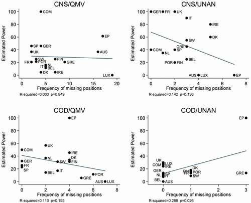
Figure 3. Estimated power and extremity (average distance), by produre.

Each panels plots power estimates from the experts range models in Table 3 against each actor’s average absolute distance from the mean positions in the DEU data.

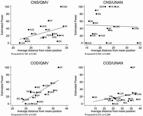
Figure 4. Estimated power and extremity (min or maxpositions), byprocedure.

Each panels plots power estimates from the experts range models in Table 3 against the percentage of times each actor took a position at the minimum or maximum of the polocy alternatives in the DEU data.

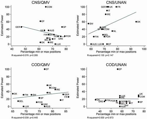
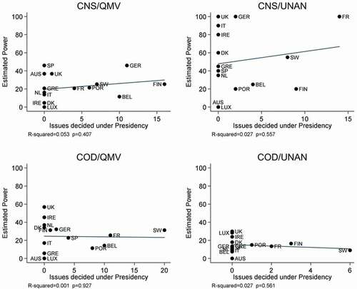
Figure 5. Estimated power and council presidency, byprocedure.

Each panel plots power estimates from the experts range models in Table 3 against the number of issues in the DEU data decided under each Member State’s Council Presidency.

For example, under CNS/QMV, Luxembourg and Austria each took by far the fewest positions, yet according to the estimates Austria is very powerful whereas Luxembourg is entirely powerless. Under CNS/UNAN, the frequency of positions is virtually identical for Denmark and Austria, yet Denmark tests out as very powerful while Austria tests out as powerless. Only under COD/UNAN does limited position taking appear to increase an actor’s power, and only if we include the European Parliament as a stark outlier.

As for spatial extremity, most studies measure this as each actor’s average absolute distance from the mean position, whereas Pajala and Widgrén (2004) operationalise it as the frequency with which each actor takes a position at the minimum or maximum of the policy alternatives. Figures 3 and 4 plot estimated power against data for both measures, which are strongly correlated only for codecision.

Again we don’t find the expected relationships. There is no indication in either Figures 3 or 4 that staking out extreme positions reduces an actor’s estimated power. In six of the eight panels, including all four in Figure 4, there appears to be no relationship between spatial extremity and estimated power. For example, under CNS/UNAN, for both measures of extremity, Austria took the least extreme positions yet tested out as powerless. Surprisingly, the two left-hand panels in Figure 3 suggest that actors who tend to take positions far from the mean Council position have significantly increased estimated bargaining power.

Finally, as shown in Figure 5, there is no evident connection between an actor’s estimated power and them holding the Council Presidency when proposals are adopted. For all four panels, R-squared values are near zero, with p > 0.4.

For example, under COD/QMV, Sweden held the Presidency far more often than did Finland or Ireland, yet according to the estimated results all three of these Member States are extremely powerful under this procedure. For CNS/UNAN, Ireland and France both test out as very powerful yet France held the Presidency more often than any other state whereas Ireland never held it.

The regression results in Figures 2–5 must be taken with caution, especially since they involve aggregating proposals by procedure, but they still clearly indicate that more work is needed to understand how it is that small Member States – and different groups of them for each procedure – apparently manage to exert so much more power than their SSI scores would predict, and why under most procedures the largest Member States are apparently so unequal and often less powerful than smaller states. The possibility that spatial extremity boosts rather than erodes an actor’s bargaining power deserves attention. Likewise, perhaps spatial extremity, focused position taking, and holding the Council Presidency operate in combination rather than individually to determine actor power. Or they might operate differently for large and small Member States, or under QMV rather than unanimity, or under consultation rather than codecision. Other factors might also be at play, such as how urgently each actor desires legislative change. Just as ‘the relative impatience of a chamber will have an effect on its influence over policy outcomes’ (Kardasheva 2013, 860), relatively impatient actors would have low power scores. The estimates might also be picking up what Bueno de Mesquita (2011) refers to as each actor’s ‘resolve’, which varies by issue but in the aggregate could vary across policy sectors and thus procedures. Finally, it might be the case that particular Member States are much more powerful in some policy sectors than others. Since each procedure tends to map on to a different sector (or sectors), and studies suggest that in practice linkage across sectors is rare, sectoral power disparities would manifest as power disparities across procedures.

Conclusion

The motivations for this article were the twin facts that formal voting power is undeniably a poor predictor of legislative decisionmaking outcomes in the European Union, and that extending previous attempts to improve the predictive accuracy of the field’s leading model by replacing formal power with estimated informal power posed daunting computational challenges. My main objective here was to offer an evolutionary computing approach that overcomes these challenges. This method opens up a range of possibilities for future research into patterns of informal power in EU decisionmaking.

An evolutionary computing approach could certainly be applied to the DEUII dataset in order to identify the power scores that best predict legislative outcomes in the post-2004 period. It is noteworthy that DEUII differs from DEU not only because it contains data on all the new states that joined as the result of two enlargements, but also because it reflects the rarity of the unanimity procedure due to treaty amendments (Thomson et al. 2012, 607). Formal power might have become a better predictor of outcomes in the enlarged EU than it was for the EU-15, or perhaps different actors now punch above or below their formal weight.

I applied an evolutionary computing approach to the compromise model because it is the leading model to date. I first extended the logic of Thomson and Hosli (2006) by optimizing unconstrained compromise models where each actor’s power could take on any value from zero to one hundred, and then fit more constrained – and arguably more plausible – models that forced each power score to fall within the range identified by expert practitioners. But a great merit of the evolutionary computing approach is that analysts can limit the solution space however they want, to make it more plausible and to test particular theories of EU power. They could, say, truncate the ranges identified by experts, or require that the largest Member States are dominant but possibly highly unequal across procedures, or that no state is more than twice as strong as any other, or that some states deploy their veto power more effectively than others, or the Commission must be at least half as strong as all of the Member States combined, or that old Member States must be stronger than new Member States, and so forth.

Finally, whereas in this paper I’ve employed the evolutionary computing approach to improve the performance of the compromise model, it might also be used to derive important cautionary lessons. For if it turns out that the only way to reduce the compromise model’s prediction errors is to allow implausible power scores, then perhaps the problem lies not in the SSI values but rather, as mentioned earlier, in the compromise model itself, or in the DEU data.

Acknowledgements

I am grateful to the two anonymous reviewers for their helpful feedback and suggestions. For their valuable comments on an early version of the paper, I thank participants at the 2014 workshop at the Netherlands Institute for Advanced Study in the Humanities and Social Sciences on “Explaining European Union Decision-Making: Insights from the Natural and the Social Sciences”. Instructions to replicate this article’s analysis, along with the data used, will be made available on the journal’s website.

Disclosure statement

No potential conflict of interest was reported by the author.

Notes

1. For example, in Bailer’s survey of expert opinions, which I discuss later, the wording of the interview question about power (2006:fn8) illustrates the interchangeability of the terms ‘power’, ‘capabilities’ and ‘influence’.

2. For greater detail see Hix and Hoyland (2011).

3. Throughout, I use ‘variant two’ SSI values, as they are referred to in the literature (Thomson and Stokman 2006, 48–49), which reflect the legal possibility that the Commission is not necessarily a member of the winning coalition.

4. Schneider, Finke, and Bailer (2010) consider a number of different bargaining models not covered in The European Union Decides, but they don’t test any of them against the compromise model, and they use imputed values for missing preferences in the DEU data which is highly problematic (Thomson 2011, 42). Thomson (2011) also tests a variety of additional bargaining models, without using imputed data, but not against the compromise model. I ran tests myself and found that for the EU-15 period, his most accurate model, a Nash Bargaining Solution that ignores the reference point, does not beat the compromise model. Bueno de Mesquita (2011) introduces a more complex and possibly superior bargaining model that includes an extra parameter for each actor’s ‘resolve’, but he appears to have used imputed data (some of his results match those of Schneider, Finke, and Bailer (2010)) which makes interpretation of his results difficult.

5. A recent regression analysis by Warntjen (2017) finds that more formal votes translate into more influence, as expected, but the study examines a different dependent variable (requested changes to Commission proposals, not bargaining success over final legislative outcomes) and uses a different pool of cases.

6. Unfortunately, their tests don’t distinguish between QMV/COD and UNAN/COD.

References

- Achen, C. 2006a. “Institutional Realism and Bargaining Models.” In The European Union Decides, edited by R. Thomson, F. Stokman, C. Achen, and T. König, 86–123. Cambridge: Cambridge University Press.
- Achen, C. 2006b. “Evaluating Political Decisionmaking Models.” In The European Union Decides, edited by R. Thomson, F. Stokman, C. Achen, and T. König, 264–298. Cambridge: Cambridge University Press.
- Aksoy, D. 2010. “““it Takes a Coalition”: Coalition Potential and Legislative Decision Making.” Legislative Studies Quarterly 35 (4): 519–542. doi:https://doi.org/10.3162/036298010793322375.
- Arregui, J. 2016. “Determinants of Bargaining Satisfaction across Policy Domains in the European Union Council of Ministers.” Journal of Common Market Studies 54 (5): 1105–1122. doi:https://doi.org/10.1111/jcms.12355.
- Arregui, J., and R. Thomson. 2009. “States’ Bargaining Success in the European Union.” Journal of European Public Policy 16 (5): 655–676. doi:https://doi.org/10.1080/13501760902983168.
- Axelrod, R. 1986. “An Evolutionary Approach to Norms.” American Political Science Review 80 (4): 1095–1111. doi:https://doi.org/10.1017/S0003055400185016.
- Bailer, S. 2004. “Bargaining Success in the European Union.” European Union Politics 5 (1): 99–124. doi:https://doi.org/10.1177/1465116504040447.
- Bailer, S. 2006. “The Dimensions of Power in the European Union.” Comparative European Politics 4 (4): 355–378. doi:https://doi.org/10.1057/palgrave.cep.6110084.
- Bueno de Mesquita, B. 2011. “A New Model for Predicting Policy Choices. Preliminary Tests.” Conflict Management and Peace Science 28 (1): 65–85. doi:https://doi.org/10.1177/0738894210388127.
- Bueno de Mesquita, B., and F. Stokman, eds. 1994. European Community Decisionmaking: Models, Applications and Comparisons. New Haven: Yale University Press.
- Cross, J. 2012. “Everyone’s a Winner (Almost): Bargaining Success in the Council of Ministers of the European Union.” European Union Politics 14 (1): 70–94. doi:https://doi.org/10.1177/1465116512462643.
- Eiben, A., and J. Smith. 2003. Introduction to Evolutionary Computing. Berlin: Springer.
- Golub, J. 2012a. “How the European Union Does Not Work: National Bargaining Success in the Council of Ministers.” Journal of European Public Policy 19: 1294–1315. doi:https://doi.org/10.1080/13501763.2012.693413.
- Golub, J. 2012b. “Cheap Dates and the Delusion of Gratification: Are Votes Sold or Traded in the EU Council of Ministers?” Journal of European Public Policy 19: 141–160. doi:https://doi.org/10.1080/13501763.2011.599996.
- Hammond, R., and R. Axelrod. 2006. “The Evolution of Ethnocentrism.” Journal of Conflict Resolution 50: 926–936. doi:https://doi.org/10.1177/0022002706293470.
- Hayes-Renshaw, F., and H. Wallace. 2006. The Council of Ministers. 2nd ed. Basingstoke: Palgrave.
- Hix, S., and B. Hoyland. 2011. The Political System of the European Union. 3rd ed. London: Palgrave.
- Hosli, M. 1996. “Coalitions and Power: Effects of Qualified Majority Voting in the Council of the European Union.” Journal of Common Market Studies 34 (2): 255–273. doi:https://doi.org/10.1111/j.1468-5965.1996.tb00571.x.
- Kardasheva, R. 2013. “Package Deals in EU Legislative Politics.” American Journal of Political Science 57 (4): 858–874.
- Larrañaga, P., C. M. H. Kuijpers, R. H. Murga, I. Inza, and S. Dizdarevic. 1999. “Genetic Algorithms for the Travelling Salesman Problem: A Review of Representations and Operators.” Artificial Intelligence Review 13 (2): 129–170. doi:https://doi.org/10.1023/A:1006529012972.
- Leinaweaver, J., and R. Thomson. 2014. “Testing Models of Legislative Decision-making with Measurement Error: The Robust Predictive Power of Bargaining Models over Procedural Models.” European Union Politics 15 (1): 43–58. doi:https://doi.org/10.1177/1465116513501908.
- Liu, Y., W. Cho, and S. Wang. 2016. “PEAR: A Massively Parallel Evolutionary Computation Approach for Political Redistricting Optimization and Analysis.” Swarm and Evolutionary Computation 30: 78–92. doi:https://doi.org/10.1016/j.swevo.2016.04.004.
- Pajala, A., and M. Widgrén. 2004. “A Priori versus Empirical Voting Power in the EU Council of Ministers.” European Union Politics 5 (1): 73–97. doi:https://doi.org/10.1177/1465116504040446.
- Panke, D. 2011. “Small States in EU Negotiations: Political Dwarfs or Power-brokers?” Cooperation and Conflict 46 (2): 123–143. doi:https://doi.org/10.1177/0010836711406346.
- Schneider, G., D. Finke, and S. Bailer. 2010. “Bargaining Power in the European Union: An Evaluation of Competing Game-Theoretic Models.” Political Studies 58: 85–103. doi:https://doi.org/10.1111/j.1467-9248.2009.00774.x.
- Selck, T., and S. Kuipers. 2005. “Shared Hesitance, Joint Success: Denmark, Finland and Sweden in the European Union Policy Process.” Journal of European Public Policy 12 (1): 157–176. doi:https://doi.org/10.1080/1350176042000311952.
- Selck, T., S. Yardimci, and C. Kathan. 2009. “Still an Opaque Institution? Explaining Decision-Making in the EU Council Using Newspaper Information: A Reply to Sullivan and Veen.” Government and Opposition 44 (4): 463–470. doi:https://doi.org/10.1111/j.1477-7053.2009.01298.x.
- Shapley, L., and M. Shubik. 1954. “A Method for Evaluating the Distribution of Power in A Committee System.” American Political Science Review 48 (3): 787–792. doi:https://doi.org/10.2307/1951053.
- Slapin, J. 2014. “Measurement, Model Testing, and Legislative Influence in the European Union.” European Union Politics 15 (1): 24–42. doi:https://doi.org/10.1177/1465116513492896.
- Tallberg, J. 2008. “Bargaining Power in the European Council.” Journal of Common Market Studies 46 (3): 685–708. doi:https://doi.org/10.1111/j.1468-5965.2008.00798.x.
- Thomson, R. (2002) “Estimation of the Relative Capabilities of the Commission, the Council and the European Parliament Using Key Informants,” 18 February, mimeo.
- Thomson, R., and F. Stokman. 2006. “Research Design, Measuring Actors Positions, Saliences and Capabilities.” In The European Union Decides, edited by R. Thomson, F. Stokman, C. Achen, and T. König, 25–53, Cambridge University Press.
- Thomson, R. 2008. “The Relative Power of Member States in the Council: Large and Small, Old and New.” In Unveiling the Council of the European Union: Games Governments Play in Brussels, edited by D. Naurin and H. Wallace, 238-258. London: Palgrave.
- Thomson, R. 2011. Resolving Controversy in the European Union. Legislative Decision-Making before and after Enlargement. Cambridge: Cambridge University Press.
- Thomson, R., F. Stokman, C. Achen, and T. König, eds. 2006. The European Union Decides. Cambridge: Cambridge University Press.
- Thomson, R., J. Arregui, D. Leuffen, R. Costello, J. Cross, R. Hertz, and T. Jensen. 2012. “A New Dataset on Decision-making in the European Union before and after the 2004 and 2007 Enlargements (DEUII).” Journal of European Public Policy 19 (4): 604–622. doi:https://doi.org/10.1080/13501763.2012.662028.
- Thomson, R., and M. Hosli. 2006. “Who Has Power in the EU? The Commission, Council and Parliament in Legislative Decision-making.” Journal of Common Market Studies 44 (2): 391–417. doi:https://doi.org/10.1111/j.1468-5965.2006.00628.x.
- Van den Bos, J. 1991. Dutch EC Policy Making: A Model-guided Approach to Coordination and Negotiation. Amsterdam: Publishers.
- Warntjen, A. 2017. “Do Votes Matter? Voting Weights and the Success Probability of Member State Requests in the Council of the European Union.” Journal of European Integration 39 (6): 673–687. doi:https://doi.org/10.1080/07036337.2017.1332057.
- Widgrén, M., and A. Pajala. 2006. “Beyond Informal Compromise: Testing Conditional Formal Procedures of EU Decision-making.” In The European Union Decides, edited by R. Thomson, F. Stokman, C. Achen, and T. König, 239–263, Cambridge: Cambridge University Press.