Extending Estimates of Tree and Tree Species Presence-Absence through Space and Time Using Landsat Composites

Abstract

We developed a methodology for extending estimates of the presence-absence of trees and several tree species contained in the Canadian National Forest Inventory using nationally consistent Landsat data products. For a prototype boreal forest region of Newfoundland and Labrador, Canada, we modeled and assessed changes in the presence-absence of trees and tree species distributions over a 25-year period. Random Forest models of presence-absence of trees had an overall classification accuracy of 0.87 ± 0.019. For five tree species, overall classification accuracies were: 0.74 ± 0.017 for balsam fir; 0.75 ± 0.028 for black spruce; 0.64 ± 0.085 for trembling aspen; 0.64 ± 0.035 for tamarack; and 0.77 ± 0.041 for white birch. While the proportion of treed area increased by 8.5% over the 25-year period, the area occupied by black spruce declined by 13.5%. The area of balsam fir and white birch increased by 9.9% and 28.2%, respectively, while trembling aspen and tamarack changed by less than 5%. The map products developed and trends observed offer baseline information in support of long-term monitoring of treed area and tree species distributions. The demonstrated methods encourage development of spatially-explicit map products to complement spatially or temporally limited forest inventory datasets.

RÉSUMÉ

Nous avons élaboré une méthodologie pour étendre les estimations de la présence-absence d’arbres et de plusieurs espèces d’arbres contenues dans l’Inventaire national des forêts du Canada à l’aide de produits Landsat normalisés à l’échelle nationale. Pour la région forestière boréale de Terre-Neuve-et-Labrador, au Canada, nous avons modélisé et évalué les changements dans la présence-absence d’arbres ainsi que dans la répartition des espèces d’arbres sur une période de 25 ans. Les modèles forestiers aléatoires de présence-absence d’arbres ont donné une précision de classification globale de 0.87 ± 0.019. Pour cinq espèces d’arbres, la classification globale était de: 0.74 ± 0.017 pour le sapin baumier; 0.75 ± 0.028 pour l’épinette noire; 0.64 ± 0.085 pour le peuplier faux-tremble; 0.64 ± 0.035 pour le mélèze; et 0.77 ± 0.041 pour le bouleau blanc. Bien que la proportion de la superficie arborée ait augmenté de 8.5% au cours de la période de 25 ans, la superficie occupée par l’épinette noire a diminué de 13.5%. La superficie du sapin baumier et du bouleau blanc a augmenté de 9.9% et de 28.2%, respectivement, tandis que celles du peuplier faux-tremble et du mélèze ont changé de moins de 5%. Les produits cartographiques élaborés et les tendances observées offrent des renseignements de base à l’appui de la surveillance à long terme des répartitions des zones arborées et des espèces d’arbres. Les méthodes présentées encouragent le développement de produits cartographiques explicites dans l’espace afin de compléter les ensembles de données spatialement ou temporellement limités sur les stocks forestiers.

Introduction

Forest inventories are essential for monitoring and reporting on the sustainability of forest resources and provide fundamental information upon which to base forest management policies and land use decisions (Corona 2016). Designed for a variety of purposes, forest inventories vary in the level of attributional and spatial detail they contain, ranging from strategic to tactical and operational information. National forest inventories are typically designed to support national and international reporting and monitoring obligations (Kangas et al. 2018), whereas tactical and operational inventories support forest management planning. As pressures on forest ecosystems increase, particularly in the context of climate change, there have been increased requirements for inventories in terms of both thematic information (Rose et al. 2015; Dyderski et al. 2018) and the level of spatial detail over large areas (Wilson et al. 2012; Hanewinkel et al. 2014). Moreover, forest inventories are employed to assess an increasing range of forest ecosystem products and services (Chirici et al. 2012; Corona 2016). Accordingly, there is a need for cost-effective inventory approaches that can be applied consistently across large areas, yet provide sufficient spatial and temporal detail to support forest management planning.

Inventory systems in Canada typically consist of the interpretation of forest stand information from aerial photographs supplemented with field data (Leckie and Gillis 1995). However, Canadian inventory systems and standards vary by province making aggregation to support forest assessments at regional to national scales difficult. Moreover, the development and application of enhanced inventory methodologies over time makes it difficult if not impossible to use these data for forest change assessments. As a result, Canada’s National Forest Inventory (NFI) was developed to support national forest policies, science initiatives, and reporting at national and international levels (Wulder et al. 2004). Canada’s NFI was designed specifically to support timely and accurate assessment and monitoring of the extent, state, and sustainable development of Canada’s forests (Gillis et al. 2005). To accommodate the large spatial extent, Canada’s NFI is based upon a systematic sample of 1% of the country, implemented using 2 km × 2 km photo-plots on a nominally 20 km × 20 km grid. While Canada’s NFI program supports reporting on forests at the national scale, it does not provide spatially-explicit maps at a level of detail needed for many applications, such as estimating timber losses from forest disturbances.

Remotely sensed data and methods are increasingly used to support inventory of forest resources over large regions (McRoberts and Tomppo 2007; Barrett et al. 2016). A variety of approaches have been used to link multiple attributes measured in forest inventories to satellite data, thus enhancing the efficiency and cost-effectiveness in mapping large forest landscapes (Kim and Tomppo 2006). Common methods such as nearest-neighbor (NN), gradient NN (Ohmann and Gregory 2002), phenological gradient nearest-neighbor (PGNN) (Wilson et al. 2012, 2013), kNN (McRoberts et al. 2005; Chirici et al. 2016), and random forests (Gislason et al. 2006; Cutler et al. 2007) use satellite imagery along with other spatial layers to map forest inventory variables. These mapping methods using medium spatial resolution optical imagery (10–100 m; e.g., from Landsat) are particularly appropriate for wall-to-wall characterization of countries like Canada with a large land base (approaching 10 million km²) and limited access to many areas (Wulder et al. 2007).

In recent studies, (Beaudoin et al. 2014, 2018) used kNN methods to map and monitor forest attributes using NFI photo plots and MODIS imagery at 250 m × 250 m spatial resolution. These map products provide valuable baseline information for strategic-level analysis of forests but do not provide the level of spatial detail needed to support operational planning. However, large area mapping projects of this nature are now possible using higher spatial resolution data sources such as Landsat (Franklin et al. 2015; Matasci et al. 2018) and Sentinel-2 (Pelletier et al. 2016; Vaglio Laurin et al. 2016). Historically, applications using Landsat data in Canada were limited by data access and the complexity associated with storing and processing large numbers of images. However, free and open access to the Landsat archive commencing in 2008 (Woodcock et al. 2008), combined with standardized and information need focused image processing procedures (White et al. 2014) supported by increased computing capabilities has resulted in Landsat best-available-pixel (BAP) products for Canada (Hermosilla et al. 2016). Value in using Landsat BAP products for forest inventory applications relates to the ability of 30 m × 30 m spatial resolution to capture fine-scale patterns of land-cover and land-use change associated with land management (Thompson et al. 2015; Hermosilla et al. 2018). Additionally, the more than 40 years of data available from Landsat sensors (White and Wulder 2014) allows for retrospective analyses including the characterization and typing of changes detected (Hermosilla et al. 2015a) and the status and trends of Canada’s forests over multiple decades at an annual time step (White et al. 2017). These advances combined with the availability of Canada’s NFI photo plot database provide standardized datasets to support the development of models linking forest attributes with satellite imagery that are consistent over large areas and through time.

The goal of this study was to develop an efficient methodology for extending forest inventory information contained in the Canadian National Forest Inventory (NFI) photo plot database across space and time using medium spatial resolution optical imagery. We focus on extending estimates of the area occupied by trees and tree species—a key information requirement for assessing potential risks and impacts of forest disturbances on resource availability and ecosystem functioning. Specific objectives were: (i) to model the presence-absence of trees and tree species using standardized datasets available within and beyond a prototype region, but commonly available for forested ecosystems across Canada; and, (ii) to monitor and assess changes in the distribution of treed area and tree species through time. Maps showing the probability of presence and/or abundance of trees and trees species inform sustainable forest management (Hudak et al. 2008) ecological modeling (Evans et al. 2011) and the assessment of ecosystem services (Vihervaara et al. 2015) while trends in species distributions provide baseline information for assessing the impacts associated with natural or anthropogenic disturbances (Pickell et al. 2016). Such assessments are increasingly important as climate change threatens to alter future distributions of tree species (Coops et al. 2010; Boucher et al. 2020). To this end, we used information contained in Canada’s NFI photo plots, Landsat BAP composites, and topographic variables to model and map the presence-absence of trees and five tree species of the boreal forest region of Newfoundland and Labrador, Canada. Further, we assessed trends in the respective tree and tree species distributions over a 25-year time period (1985–2010).

Material

Study Area

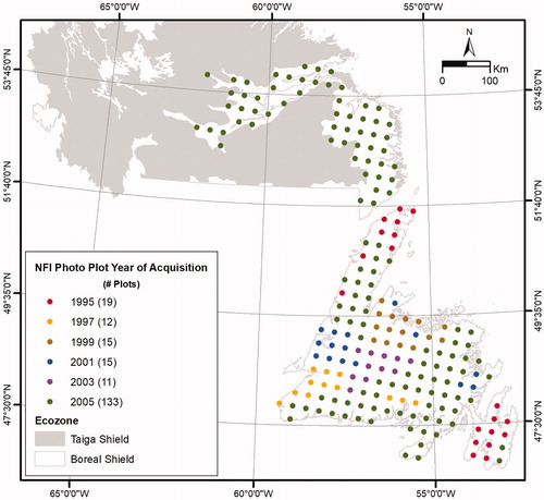
The 15.7 million hectare study area encompassed the boreal forest of Newfoundland and Labrador, Canada (Figure 1). These forests represent the eastern extent of the boreal forest region of North America (Rowe 1972) and are dominated by coniferous vegetation with balsam fir (Abies balsamea (L.) Mill.) and black spruce (Picea mariana (Mill.) B.S.P.) as the most common tree species. Fir stands dominate the western, northern and eastern regions of the island, whereas spruce stands dominate the central region of the island and Labrador (Government of Newfoundland and Labrador 2019). Tamarack (Larix laricina (DuRoi) K. Koch) are found mostly in swampy, wet places while other species that represent significant components of mixed wood and hardwood stands on the island include white birch (Betula papyrifera (Marshall)) and trembling aspen (Populus tremuloides (Michaux F.). White spruce (Picea glauca (Moench) Voss) may be found on more favorable sites, while red pine (Pinus resinosa (Ait.)) are situated mainly in small isolated stands. Average annual temperatures on the island range from −3 to 10 degrees C and average yearly precipitation ranges from 952 to 1686 mm (Osborn 2019). Labrador annual temperatures are cooler ranging from −9 to 5 degrees C with average yearly precipitation from 840 to 1073 mm (Osborn 2019).

Figure 1. Distribution of National Forest Inventory photo plots by year of aerial photography acquisition within the Boreal Shield Ecozone of Newfoundland and Labrador, Canada.

NFI Photo Plots and Measurement Protocol (Response Variables)

NFI photo plot data representing the period from 1995 to 2005 (Figure 1) consisted of forest stands interpreted from aerial photography and characterized by a suite of attributes describing the land cover, land use, ownership and protection status (National Forest Inventory 2008). Crown closure represented the percent ground area in the stand that was covered by the vertical projection of all tree crowns in the polygon. A polygon was considered to be treed if crown closure was 10% or greater (National Forest Inventory 2008). Photo interpreters also recorded species’ relative proportions as determined by the percentage of stand basal area per hectare.

Predictor Variables for Species Modeling

We selected a combination of layers to represent factors influencing the presence-absence of trees and tree species including: annual spectral variables characterizing vegetation and topographic variables characterizing moisture regimes and solar radiation effects (Table 1). We derived spectral variables from Landsat BAP proxy surface reflectance composites (Hermosilla et al. 2016). The annual BAP composites contained the best available pixel observation (from a target year) for any given pixel location. BAP proxy composites were produced for the years 1984–2012 using a set of specified rules that included a day-of-year rule limiting pixels to a phenological window of August 1 ± 30 days (White et al. 2014). If there were no observations that satisfied the compositing rules for a given pixel location, the pixel was coded as “no data”. The “no data” observations were infilled with proxy values using pixel-level time series information according to the methods described in Hermosilla et al. (2015b); however, infilled pixels were excluded from all of our analysis. The BAP proxy composites each contained 6 surface reflectance bands: Blue, Green, Red, NIR, SWIR, and SWIR2 (e.g., true color illustration, Figure 2). From the spectral bands, we derived tasseled cap transformations representing brightness (TCBRI), greenness (TCGRE), and wetness (TCWET) and other spectral indices including the enhanced vegetation index (EVI), modified soil adjustment index (MSAVI), normalized difference moisture index (NDMI) and normalized difference vegetation index (NDVI). These indices correspond to the physical characteristics of vegetation (Banskota et al. 2014) and are commonly used for studying forest change (Cohen et al. 2002; Healey et al. 2005). They are less sensitive to atmospheric effects than the original bands (Song and Woodcock 2003) and are often used to reduce data dimensionality (Song et al. 2007). We gridded Canadian Digital Elevation Model (CDEM) elevation data to a 30 m × 30 m resolution. CDEM data is derived mainly from elevation contours and hydrographic data at a scale of 1:50,000, with a base resolution of 0.75 arc seconds (∼23 m) in the north-south (Government of Canada 2017). We derived slope and aspect from the elevation data using ESRI ArcGIS 10.4.1 (ESRI 2016). In addition, we generated transformations of slope combined with aspect (SCOSA and SSINA) to represent how solar radiation varies across the landscape (Stage 1976).

Figure 2. Illustration of a Landsat BAP true color proxy composite image (RGB = Bands 4, 3, 2) for 2003.

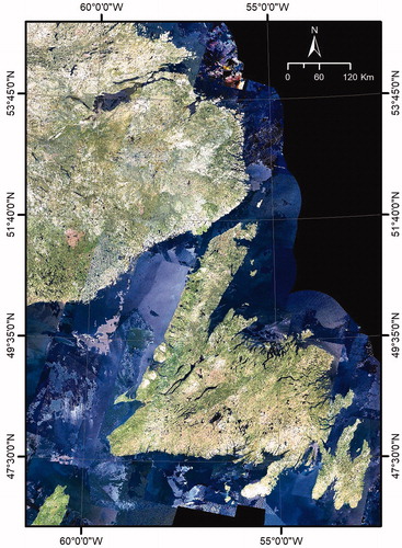
Table 1. Description of predictor variables.

	Description	Reference
Spectral Variables
TCBRI	Tasseled Cap Brightness	Crist 1985
TCGRE	Tasseled Cap Greenness	Crist 1985
TCWET	Tasseled Cap Wetness	Crist 1985
EVI	Enhanced Vegetation Index	USGS 2014
MSAVI	Modified Soil Adjusted Vegetation Index	USGS 2014
NDMI	Normalized Difference Moisture Index	USGS 2014
NDVI	Normalized Difference Vegetation Index	USGS 2014
Topographic Variables
Slope	Slope (%)
Elevation	Elevation (m)	Government of Canada 2017
SCOSA	Slope * cosine (aspect) transformation	Stage 1976
SSINA	Slope * sine (aspect) transformation	Stage 1976

Methods

Data Preparation

The first step of our methodology for extending the presence-absence of trees and tree species across space and time (Figure 3) involved preparing a multi-year database of predictor and response variables. First, we projected the NFI photo plot layers and the topographic data to the UTM NAD83 21 N coordinate system and resampled the topographic data to align with the Landsat BAP composites (30 m × 30 m). Then, we extracted the response variables (presence-absence of trees and each tree species) at the stand level from the NFI photo plot data. We calculated the predictor variables as stand-wise averages of all pixels located within NFI polygons excluding a 30 m buffer applied to the boundary of each NFI polygon and excluding proxy pixels which included infilled data. For the spectral predictors, we selected Landsat BAP proxy composites to correspond to the year of air photo acquisition for the NFI photo plot in order to minimize the possibility of selecting pixels that might have changed since the time of air photo acquisition. The resulting database contained an exhaustive list of all potential sample points (one for each NFI polygon) with the response variables derived from the NFI photo plots (tree and tree species presence-absence) and the predictor variables (spectral and topographic) derived from the spatially comprehensive layers.

Figure 3. Methodology for extending tree presence-absence and individual tree species presence-absence information through space and time (R package indicated in brackets).

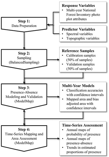
Sampling

We used a stratified sampling approach to randomly select samples for calibration and validation of each model, whereby strata were defined as the presence-absence of trees and individual tree species. We chose sample sizes according to the availability of potential sample points within each stratum (Table 2). We used the local pivotal method of sampling (lpm2_kdtree) found within the BalancedSampling package (Grafström and Lisic 2019) in R (R Core Team 2019) to maximize the range of spatial, topographic and spectral variability in the sample points. We used longitude and latitude variables to achieve spatial balance and elevation to achieve topographic balance. We selected spectral balancing variables for each species as the most important variable as determined by preliminary random forest models. The minimum distance between samples selected for each response variable was 60 m. We randomly split the selected samples for model calibration and validation. We used a 50/50 split to balance the variation between predicted estimates and model performance statistics because we favored a more generalized model over a more specialized (over-fit) model that might occur with a higher proportion of calibration samples. We did not model red pine and white spruce as these species were represented by fewer than 100 samples, and preliminary tests indicated that models developed for these infrequently occurring species resulted in over-prediction across the landscape.

Table 2. Model sample sizes, thresholds, and sensitivity and specificity values.

Model	Species	n (calibration)	n (validation)	Threshold	Sensitivity	Specificity
Tree Presence-Absence		1250	1250	0.5	0.87	0.87
Species Presence-Absence	Balsam fir	2500	2500	0.51	0.74	0.74
	Black spruce	1000	1000	0.53	0.75	0.75
	Trembling aspen	150	150	0.56	0.64	0.64
	Tamarack	750	750	0.49	0.64	0.64
	White birch	500	500	0.53	0.77	0.77

Threshold: user specified threshold to define presence-absence using predicted probability; Sensitivity: TP/(TP + FN) with TP as true positives and FN as false negatives; Specificity: TN/(TN + FP) with TN as true negatives and FP as false positives.

Presence-Absence Modeling and Validation

We built random forest models of the presence-absence of trees and individual tree species (response variables) and predicted the probability of presence for areas that were unknown using spatially comprehensive layers (predictor variables). We built the random forest models in R (R Core Team 2019) with the ModelMap package (Freeman and Frescino 2009). ModelMap automates the process of model building and map construction by providing an interface with several R packages including: randomForest (Liaw and Wiener 2002). We developed all models using the default of 500 decision trees and using the tuneRF function from the randomForest package to optimize the number of explanatory variables for each split (mtry). We limited the species models and associated predictions to areas that were treed.

We defined thresholds for presence that balanced sensitivity and specificity according to the reference data (Table 2), whereby sensitivity is the ability of a model to detect a species when it is present and specificity is the ability of a model to not predict a species when it is absent (Fielding and Bell 1997; van der Maaten et al. 2017). We estimated user’s accuracy (or commission error), producer’s accuracy (or omission error), overall accuracy and associated confidence intervals using estimated area proportions corresponding to the mapped classes as recommended by (Olofsson et al. 2014). We further estimated area proportions of presence-absence based on the reference classification and quantified uncertainty in the area estimates following the procedures also explained in (Olofsson et al. 2014).

Time-Series Mapping and Area Assessment

We produced annual maps of the probability of presence by applying the models developed with multi-year training data to each year of the Landsat BAP composite time-series using ModelMap. Since the models were developed using surface reflectance and similar phenology (i.e., BAP date range of August 1 ± 30 days), the models were eligible for application to any year of imagery regardless of when the training data were collected (Song et al. 2001; Fekety et al. 2015). We subsequently classified the model predictions of probability of presence into binary classes of presence-absence according to the selected thresholds. Finally, we calculated proportions of presence from the mapped areas, and we corrected the mapped proportions for classification bias (Olofsson et al. 2014). We plotted the bias-correct proportions to show trends in the presence of tree and individual trees species areas over the 25-year time period.

Results

Model Accuracy and Uncertainty

The presence-absence model of trees had an overall accuracy of 0.87 ± 0.019 (Table 3). User’s accuracies were 0.88 ± 0.025 and 0.87 ± 0.27% for presence and absence, respectively. Producer’s accuracies were 0.92 ± 0.019 (presence) and 0.83 ± 0.016 (absence). The individual species models predicted the presence-absence of each species with overall accuracies ranging from a high of 0.78 ± 0.039 for white birch and a low of 0.63 ± 0.083 for trembling aspen. The remaining species had overall accuracies of 0.75 ± 0.028 for black spruce, 0.74 ± 0.017 for balsam fir, and 0.64 ± 0.035 for tamarack. User’s accuracies for the presence of individual species ranged from 0.77 ± 0.052 for white birch to 0.63 ± 0.049 for tamarack, while producer’s accuracies ranged from 0.83 ± 0.023 for black spruce to 0.44 ± 0.086 for trembling aspen.

Table 3. Error matrices populated by estimated proportions of area and stratified estimators of accuracy.

	Reference
	Presence	Absence	Total	Area (pixels)	User’s accuracy
Mapped
Treed
Presence	0.521	0.071	0.592	443928	0.88 ± 0.025
Absence	0.055	0.354	0.408	306529	0.87 ± 0.027
Total	0.576	0.424	1.000	750457
Producer’s accuracy	0.91 ± 0.017	0.83 ± 0.016
Overall accuracy	0.87 ± 0.019
Balsam fir
Presence	0.400	0.133	0.533	236500	0.75 ± 0.024
Absence	0.125	0.342	0.467	207428	0.73 ± 0.025
Total	0.525	0.475	1.000	443928
Producer's accuracy	0.76 ± 0.018	0.72 ± 0.017
Overall accuracy	0.74 ± 0.017
Black spruce
Presence	0.456	0.157	0.613	272298	0.74 ± 0.038
Absence	0.093	0.293	0.387	171630	0.76 ± 0.038
Total	0.549	0.451	1.000	443928
Producer's accuracy	0.83 ± 0.023	0.65 ± 0.02
Overall accuracy	0.75 ± 0.028
Trembling aspen
Presence	0.197	0.115	0.311	138203	0.63 ± 0.109
Absence	0.251	0.437	0.689	305725	0.64 ± 0.11
Total	0.448	0.552	1.000	443928
Producer's accuracy	0.44 ± 0.086	0.79 ± 0.139
Overall accuracy	0.63 ± 0.083
Tamarack
Presence	0.245	0.141	0.386	171520	0.63 ± 0.049
Absence	0.222	0.392	0.614	272408	0.64 ± 0.049
Total	0.467	0.533	1.000	443928
Producer's accuracy	0.52 ± 0.039	0.73 ± 0.05
Overall accuracy	0.64 ± 0.035
White birch
Presence	0.239	0.070	0.308	136951	0.77 ± 0.052
Absence	0.153	0.538	0.692	306977	0.78 ± 0.052
Total	0.392	0.608	1.000	443928
Producer's accuracy	0.61 ± 0.058	0.89 ± 0.082
Overall accuracy	0.78 ± 0.039

The mapped treed proportion of the total NFI plot area was 0.592, whereas the bias-corrected proportion was 0.576 ± 0.019. These proportions corresponded to a mapped area of 443928 pixels and a bias-corrected treed area of 431967 ± 31908 pixels (Table 4). The species with the highest estimated area of presence was black spruce (243904 ± 12247 pixels) followed by balsam fir (232889 ± 7628 pixels), tamarack (207328 ± 15707 pixels), trembling aspen (198834 ± 36980 pixels) and white birch (174054 ± 174313 pixels). According to the reference data, the mapped areas derived from pixel counting overestimated the proportion of treed area by 0.016. The most common species proportions were overestimated by 0.008 (balsam fir) and 0.064 (black spruce), while the less common species were underestimated by 0.137 (trembling aspen), 0.081 (tamarack), and 0.084 (white birch).

Table 4. Mapped area and adjusted area with uncertainty estimates derived with the reference data.

	Mapped Data		Reference Data
	Map proportion	Map area (pixels)	Estimated proportion	Estimated area (pixels)
Treed
Presence	0.592	443928	0.576 ± 0.019	431967 ± 13908
Absence	0.408	306529	0.424 ± 0.019	318490 ± 13908
Total	1.000	750457
Balsam fir
Presence	0.533	236500	0.525 ± 0.017	232889 ± 7628
Absence	0.467	207428	0.475 ± 0.017	211039 ± 7628
Total	1.000	443928
Black spruce
Presence	0.613	272298	0.549 ± 0.028	243904 ± 12247
Absence	0.387	171630	0.451 ± 0.028	200024 ± 12247
Total	1.000	443928
Trembling aspen
Presence	0.311	138203	0.448 ± 0.083	198834 ± 36980
Absence	0.689	305725	0.552 ± 0.083	245094 ± 36980
Total	1.000	443928
Tamarack
Presence	0.386	171520	0.467 ± 0.035	207328 ± 15707
Absence	0.614	272408	0.533 ± 0.035	236600 ± 15707
Total	1.000	443928
White birch
Presence	0.308	136951	0.392 ± 0.039	174054 ± 17413
Absence	0.692	306977	0.608 ± 0.039	269874 ± 17413
Total	1.000	443928

Annual Maps and Trends

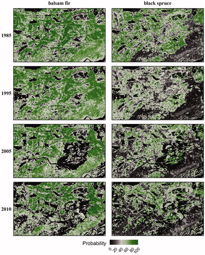
Annual map products generated with the random forest models show predicted probability of presence and also presence and absence areas according to the applied thresholds (e.g., Figure 4). Forest harvesting occurred in this particular area circa 2005 and is visible in both the probability of presence and the presence-absence maps with the threshold applied. Similarly, annual map products include the predicted probability of presence and associated presence-absence maps of individual tree species (e.g., Figure 5). The individual species maps illustrate a higher probability of balsam fir presence as compared to black spruce in the western Newfoundland region shown.

Figure 4. Probability of presence and binary map of treed and non-treed area created using a threshold of 0.5 for a selected area in western Newfoundland, Canada. Area of forest harvesting circled in red.

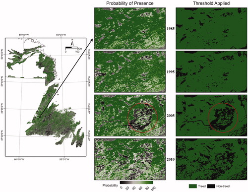
Figure 5. Probability of presence of the 2 most common tree species for a selected area in western Newfoundland, Canada.

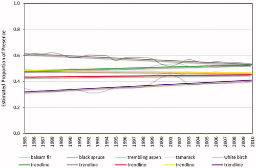
For the 25-year time period, the bias-corrected proportion of the treed area ranged from 0.53 to 0.61 with an average of 0.58 and an overall increase of 8.5% (Figure 6). The predicted presence of black spruce exhibited a downward trend with proportions ranging from a high of 0.62 to a low of 0.52 and an overall decrease of 13.5% (Figure 7). Balsam fir and white birch showed upward trends with overall increases of 9.9% and 28.2%, respectively, while tamarack and trembling aspen remained relatively stable changing by less than 5% over the 25 years.

Figure 6. Estimated proportion of the total NFI photo plot area that was treed.

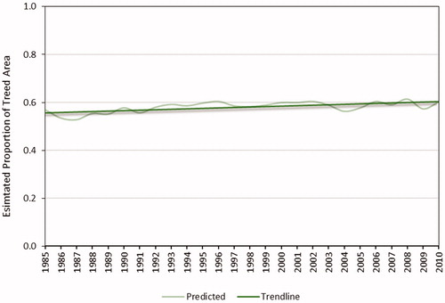
Figure 7. Estimated proportion of the treed NFI photo plot area for each species.

Discussion

Prediction of Tree Presence-Absence Distributions

The model of tree presence-absence developed with multi-year NFI photo plot data predicted the presence of trees with high accuracy based on an assessment of withheld NFI sample plots (overall accuracy 0.87 ± 0.019). Estimates of percent treed area derived from the model predictions and corrected for bias for each year were within ± 3.4% of the fit line (Figure 6). Annual fluctuations may have resulted from poor image quality in some years (e.g., cloud/haze was evident in the 1987, 2000 and 2004 composites), with extended periods of cloud cover and haze common in Newfoundland and Labrador (White et al. 2014). Nonetheless, Banskota et al. 2014 note that approaches using time-series data are generally robust toward minor reflectance perturbations. In this case, a single multi-year model was applied to each year of the Landsat BAP data. Although estimates for a single year may be influenced by image quality, the overall trends are less sensitive to annual perturbations. For the time period corresponding to the NFI photo plots (1995–2005), the estimated proportion of tree presence derived from the model predictions was 0.59. The general statistic of treed area reported by the government department responsible for forest management is also 0.59 (Government of Newfoundland and Labrador 2014).

The estimated increase in treed area over the 25-year time period from 1985–2010 may be explained as a consequence of the disturbance history of the region. The island portion of Newfoundland experienced the largest spruce budworm outbreak on record during 1972–1992, and 1986 was a major fire year (Arsenault et al. 2016). Many areas affected by these disturbances experienced regeneration during 1985–2010, which likely contributed to the gradual increase in the overall treed area. However, trends vary across different regions depending on the timing and nature of disturbance. For example, in the Humber River Basin of western Newfoundland, van Lier et al. (2011) reported a decrease in treed area for the period 1990–2007 corresponding with industrial forest harvesting.

Prediction of Tree Species Presence-Absence Distributions

The individual tree species models had variable accuracies with the most commonly occurring species generally having higher overall accuracies (balsam fir: 0.74 ± 0.017, black spruce: 0.75 ± 0.023, white birch: 0.78 ± 0.039) than the less common species (trembling aspen: 0.63 ± 0.083, tamarack: 0.64 ± 0.035). The exception was white birch with the highest overall classification (0.78 ± 0.039) but the lowest estimated area of presence. Balsam fir and black spruce in Newfoundland and Labrador tend to occur in more homogenous forest stands which have been shown to provide better training data compared to training data derived from more heterogeneous stands (Šebeň and Bošeľa 2010; Shao and Lunetta 2012). Photo interpretation errors also tend to be lower for pure conifer stands compared to mixedwood stands (Potvin et al. 1999), and higher accuracies tend to occur for forest types comprised of one or two species (Thompson et al. 2007). Tamarack, a deciduous conifer, has a spectral signature that resembles those of broadleaved trees which can cause confusion for spectral based models (Hovi et al. 2017; Rautiainen et al. 2018). Also, tamarack is commonly found on stand edges or within heterogeneous stands making classification challenging because many tree species have overlapping spectral reflectance characteristics (Thompson et al. 2015). Trembling aspen is found in smaller more localized geographic areas and thus had fewer samples for model calibration and validation. Previous studies have demonstrated that developing predictive models with small sample sizes can affect classification accuracy (Fassnacht et al. 2014; Sousa Da Silva et al. 2020).

We report trends in individual species distributions over time for the overall study area. We observed an overall decrease in black spruce presence (13.5%) and overall increases in balsam fir (9.9%) and white birch presence (28.1%). On more productive sites, black spruce does not compete successfully with balsam fir and other species (Viereck and Johnston 1990). As a result, black spruce forests that are clearcut often regenerate to other species or fail to regenerate without the aid of expensive site preparation. On the island of Newfoundland, harvested black spruce stands frequently regenerate naturally as balsam fir without planting intervention (Brown et al. 2011). Lack of seed supply, lack of sufficient area of good seedbed media, and an increased occurrence of Kalmia angustifolia were identified as limiting factors for black spruce regeneration (van Nostrand 1971). In Labrador, Elson et al. (2007) found a greater proportion of balsam fir following the harvest of black spruce stands as a result of understory balsam fir persisting after the overstory had been logged.

In contrast to clearcut logging, fire usually destroys hardwood and balsam fir understories (Bergeron et al. 1999; McRae et al. 2001). While fire is known to promote black spruce regeneration (Brown et al. 2011), post-fire regeneration can be affected by other factors such as fire intensity and site quality (Mallik 2003). After wildfires, black spruce stands may initially regenerate as pioneer tree species other than black spruce, especially on high quality sites in Newfoundland where regeneration from softwood to white birch is common (Brown et al. 2011). After forest canopy removal, the regeneration of black spruce may also be inhibited by increases in Kalmia angustifolia cover (Mallik 2003). In Labrador, Elson et al. (2007) found an absence of black spruce on burned sites supporting an argument by (Foster 1985) that low fire frequency may result in an accumulation of organic matter which provides a poor seed bed for black spruce. The study by Simon and Schwab (2005) further supports the idea that charred duff that is incompletely removed by fire results in slow regeneration. While an assessment of the impacts of various types and intensities of disturbance on species regeneration was beyond the scope of this study, the overall trends observed—decline in black spruce with corresponding increases in balsam fir and white birch—are not surprising for this boreal forest region of eastern Canada.

Data and Technical Considerations

In any modeling exercise, quality of the data is an important consideration (Vega Isuhuaylas et al. 2018). The results achieved in this study were dependent on the quality of the presence-absence data as well as the spatially comprehensive data used for both model development and application. While data quality of the response variables influenced the models explanatory power, the quality of the predictor variables affected both the quality of the models and the reliability of the model predictions (Stockwell and Peterson 2002; Zaniewski et al. 2002). The response data (presence-absence) was derived from a nationally standardized database of NFI photo plots. Although field measurements are normally preferred over interpretations from aerial photographs for model development, the advantage of using NFI photo plots for this study was that they were spatially well-distributed and captured the variability in both the dependent and independent variables. This data characteristic was critical to ensure that derived models provide an adequate representation of the ecological niche and are capable of landscape level prediction (Evans et al. 2011). Further, the NFI photo plots contained both presence and absence data. Generally, if absence data are available, methods using presence-absence information are preferred over presence-only methods in most situations (Brotons et al. 2004). Good quality presence-absence data are necessary for generating quality statistical models. While the quality of photo-interpreted data is known to be affected by interpreter skill level, photo quality, time of year, minimum mapping unit, and positional accuracies (Leckie and Gillis 1995; Magnussen and Russo 2012), the photo-interpreted presence-absence data for the dominant species of this study were assumed to be reliable given the experience of the interpreters and the relatively homogeneous coniferous forest conditions of Newfoundland and Labrador. The interpretations of non-dominant species and those that occur less frequently may have been less reliable.

The predictor variables were derived from Landsat BAP proxy composites (Hermosilla et al. 2016). The BAP proxy composites are gap-free, radiometrically and phenologically consistent composites available for Canada representing the time period of our study. Our assumption was that the BAP image products had consistent radiometry over time. However, many factors may influence the radiometric quality of the BAP time-series products including sensor issues, data availability, and data preprocessing (reviewed in Banskota et al. (2014)). While atmospheric conditions contributed to errors in BAP products for some years (i.e., limited image data yield due to cloud, shadow, and haze), such inconsistencies had minimal effect on the overall trends observed. The advantage of using multi-year BAP composites of surface reflectance values was that the spectral data could be extracted for the specific year corresponding to the NFI photo plot. Moreover, surface reflectance values allow for the extension of models in both time and space (Song et al. 2001). Since a single model was developed with photo plots from multiple years and the same model was applied to each year of the Landsat BAP time series, any trends observed were not due to differences in model parameterization across different years.

We selected the random forest algorithm (Breiman 2001) to model the complex ecological interactions among predictor variables and to predict presence-absence while avoiding the assumptions of conventional parametric modeling techniques (Elith and Leathwick 2009; Evans and Cushman 2009). We selected random forest because this approach is especially suited when the goal of an analysis is prediction over formal explanation of hypotheses (Evans et al. 2011) and because issues related to parametric statistics (e.g., assumptions of normality) and other classification and regression tree approaches (e.g., over-fitting and bias) are reduced (Brosofske et al. 2014). Other machine learning algorithms have been used successfully for land cover classifications such as support vector machine (SVM), however, the selection of the kernel parameters can be challenging (Zafari et al. 2019). Additionally, classification and regression trees (CART) have been used (Shao and Lunetta 2012), but these algorithms are limited to a single regression tree whereas random forest creates multiple trees based on a bootstrapped sample of data and then combines predictions. To model individual tree species, we adopted the strategy of modeling distributions of each species one at a time (Guisan and Thuiller 2005). We modeled each species individually and subsequently classified the probability of presence as present or absent. It has been hypothesized that a community approach to modeling may offer advantages over individual species modeling, because it takes into account co-occurrence of species and includes species that may have limited data (Elith et al. 2006; Bonthoux et al. 2013). Alternate modeling approaches are worthy of further investigation to evaluate if there are benefits to be gained with assemblage modeling over the modeling of individual species presence-absence.

Regarding the evaluation of the models and model predictions, the capability of statistical tools to accurately model species distributions is difficult to evaluate fully, in part because the NFI photo plot data does not necessarily represent “truth”. While precise ground plot data would have been preferred for model evaluation, data-collection efforts in Newfoundland and Labrador were not comprehensive enough to provide sufficiently distributed and standardized ground plot data for modeling or independent model evaluation. The NFI photo plot data that was available spanned multiple years and was limited to the period 1995–2005, therefore it was not possible to evaluate the classification accuracy of maps produced for years without NFI photo plots. None-the-less, we were able to use the NFI reference data to assess the magnitude of bias and correct area estimates associated with the multi-year models. Furthermore, given that NFI photo plot data were not available beyond the first measurement period (1995–2005) for our study area, we could not assess trends from the NFI photo plot data to compare with the temporal trends derived from the Landsat BAP composites. Such assessments may be possible when NFI photo plot remeasurements become available in the future. (Canada’s National Forest Inventory 2016).

Originality of the Approach

The originality of the approach is in the use of multi-year NFI plot data and multi-year Landsat data for model development, time-series mapping and area assessment. We developed models that could be applied to annual Landsat BAP composites derived from surface reflectance of similar phenology. We used the models to produce annual maps of the boreal forest of Newfoundland and Labrador which would be impossible to do with aerial photography and reference data alone. The annual map products provide a single area estimate for each class that is subject to classification bias. Correcting the annual areal proportions derived from the maps for bias allowed us to analyzed trends in tree cover and tree species presence over a 25 year period. Since the methodology was developed with nationally consistent data sets, it has the potential to be evaluated and applied at a national scale across Canada. With satisfactory results, the method could have high practical value for Canadian forest management, science, and policy.

Implications for Forest Inventory and Monitoring

While forest inventories require information on a broad suite of forest attributes, in this study, we focused on the presence of trees and tree species as forest managers and policy makers require such information in order to assess long-term impacts of natural and anthropogenic disturbance. The methodology could potentially be applied to other attributes characterizing forest structure and species abundance if the photo plot data for a given attribute were found to be sufficiently precise. Clearly, a limitation of our study was the lack of information on species abundance. This was in part due to the difficulty of reliably assigning abundance values to the photo interpretation of species. While the mapping and monitoring methodology offered in this study can be considered to be relatively low-cost, it is limited to those attributes that can be reliably interpreted or modeled in NFI photo plots with sufficient precision. Clearly, a tradeoff lies between the cost of a methodology and the quality of the information it provides (Legg and Nagy 2006).

Lastly, this study methodology was developed for a prototype region representing the boreal forest of Newfoundland and Labrador. Locally, the results may be used to provide insights on the long-term impacts of natural and anthropogenic disturbances on tree presence-absence and individual tree species distributions. Applying the methodology beyond the boreal forest region of Newfoundland and Labrador requires further evaluation of the applicability of the methodology to more complex and mixed forest conditions.

Conclusions

This study presents an efficient methodology for extending inventory information contained in the current Canadian NFI monitoring system across space and time using nationally consistent Landsat BAP products. Random forest models for predicting the presence-absence of trees had an overall classification accuracy of 0.87 ± 0.019. For five tree species, overall classification accuracies were: 0.74 ± 0.017 for balsam fir; 0.75 ± 0.028 for black spruce; 0.64 ± 0.085 for trembling aspen; 0.64 ± 0.035 for tamarack; and for 0.77 ± 0.041 white birch. For the boreal forest region of Newfoundland and Labrador, Canada, the estimated proportion of area occupied by trees increased by 5%, while the proportion of the primary commercial species, black spruce, declined by 8% over the 25-year time period analyzed (1985–2010). Balsam fir and white birch proportions increased by 5% and 9%, respectively, while the less common species of trembling aspen and tamarack changed by less than 2%. As pressures on forest ecosystems continue to increase, the map products and trends observed offer baseline information in support of long-term monitoring of tree presence-absence and species distributions.

The results presented in this study are for the boreal forest region of Newfoundland and Labrador, Canada. However, the use of standardized NFI photo plots and multi-year Landsat BAP products allow for portability of the methods to other regions of Canada. In fact, multi-year models could be developed from any forest inventory plot program that involves plot data collection (aerial or ground) spanning multiple years. Further evaluation of the methodology for mapping and assessing trends in other forest attributes is also possible.

Acknowledgements

This research was carried out under the “National Terrestrial Ecosystem Monitoring System (NTEMS): Timely and detailed national cross-sector monitoring for Canada” project jointly funded by the Canadian Space Agency (CSA) Government Related Initiatives Program (GRIP) and the Canadian Forest Service (CFS) of Natural Resources Canada. The NFI design and plot database was a result of collaboration among the federal, provincial and territorial governments across Canada. We thank Glenn Luther for statistical advice, Dr. Txomin Hermosilla and Geordie Hobart of the Canadian Forest Service for generating the Landsat BAP composites, and the NFI team, including staff members at the CFS’s NFI Project Office and partners at the Newfoundland Department of Natural Resources for providing access to the NFI photo plot database.

Disclosure statement

No potential conflict of interest was reported by the author(s).

References

- Arsenault, A., LeBlanc, R., Earle, E., Brooks, D., Clarke, B., Lavigne, D., and Royer, L. 2016. “Unravelling the past to manage Newfoundland’s forests for the future.” The Forestry Chronicle, Vol. 92 (No. 4): pp. 487–502. doi:10.5558/tfc2016-085.
- Banskota, A., Kayastha, N., Falkowski, M.J., Wulder, M.A., Froese, R.E., and White, J.C. 2014. “Forest monitoring using landsat time series data: A review.” Canadian Journal of Remote Sensing, Vol. 40 (No. 5): pp. 362–384. doi:10.1080/07038992.2014.987376.
- Barrett, F., McRoberts, R.E., Tomppo, E., Cienciala, E., and Waser, L.T. 2016. “A questionnaire-based review of the operational use of remotely sensed data by national forest inventories.” Remote Sensing of Environment, Vol. 174: pp. 279–289. doi:10.1016/j.rse.2015.08.029.
- Beaudoin, A., Bernier, P.Y., Guindon, L., Villemaire, P., Guo, X.J., Stinson, G., Bergeron, T., Magnussen, S., and Hall, R.J. 2014. “Mapping attributes of Canada’s forests at moderate resolution through k NN and MODIS imagery.” Canadian Journal of Forest Research, Vol. 44 (No. 5): pp. 521–532. doi:10.1139/cjfr-2013-0401.
- Beaudoin, A., Bernier, P.Y., Villemaire, P., Guindon, L., and Guo, X.J. 2018. “Tracking forest attributes across Canada between 2001 and 2011 using a k nearest neighbors mapping approach applied to MODIS imagery.” Canadian Journal of Forest Research, Vol. 48 (No. 1): pp. 85–93. doi:10.1139/cjfr-2017-0184.
- Bergeron, Y., Harvey, B., Leduc, A., and Gauthier, S. 1999. “Forest management guidelines based on natural disturbance dynamics: Stand- and forest-level considerations.” The Forestry Chronicle, Vol. 75 (No. 1): pp. 49–54. doi:10.5558/tfc75049-1.
- Bonthoux, S., Baselga, A., and Balent, G. 2013. “Assessing Community-Level and Single-Species Models Predictions of Species Distributions and Assemblage Composition after 25 Years of Land Cover Change.” PLoS One, Vol. 8 (No. 1): pp. e54179. doi:10.1371/journal.pone.0054179.
- Boucher, D., Gauthier, S., Thiffault, N., Marchand, W., Girardin, M., and Urli, M. 2020. “How climate change might affect tree regeneration following fire at northern latitudes: A review.” New Forests, Vol. 51 (No. 4): pp. 543–571. doi:10.1007/s11056-019-09745-6.
- Breiman, L. 2001. “Random Forests.” Machine Learning, Vol. 45 (No. 1): pp. 5–32. doi:10.1023/A:1010933404324.
- Brosofske, K.D., Froese, R.E., Falkowski, M.J., and Banskota, A. 2014. “A review of methods for mapping and prediction of inventory attributes for operational forest management.” Forest Science, Vol. 60 (No. 4): pp. 733–756. doi:10.5849/forsci.12-134.
- Brotons, L.L., Thuiller, W., Araujo, M.B., Hirzel, A.H., Araújo, M.B., and Hirzel, A.H. 2004. “Presence-Absence versus Presence-Only Modelling Methods for Predicting Bird Habitat Suitability.” Ecography, Vol. 27 (No. 4): pp. 437–448. doi:10.1111/j.0906-7590.2004.03764.x.
- Brown, W., Wells, D., and Wells, E.D. 2011. The Pre-Industrial Condition of the Forest Limits of Corner Brook Pulp and Paper Limited. Corner Brook, NL.
- Canada’s National Forest Inventory [online]. 2016. Available from: https://nfi.nfis.org/en/ [Accessed 5 Apr 2019].
- Chirici, G., McRoberts, R.E., Winter, S., Bertini, R., Brändli, U.-B., Asensio, I.A., Bastrup-Birk, A., Rondeux, J., Barsoum, N., and Marchetti, M. 2012. “National forest inventory contributions to forest biodiversity monitoring.” Forest Science, Vol. 58 (No. 3): pp. 257–268. doi:10.5849/forsci.12-003.
- Chirici, G., Mura, M., McInerney, D., Py, N., Tomppo, E.O., Waser, L.T., Travaglini, D., and McRoberts, R.E. 2016. “A meta-analysis and review of the literature on the k-nearest neighbors technique for forestry applications that use remotely sensed data.” Remote Sensing of Environment, Vol. 176: pp. 282–294. doi:10.1016/j.rse.2016.02.001.
- Cohen, W.B., Spies, T.A., Alig, R.J., Oetter, D.R., Maiersperger, T.K., and Fiorella, M. 2002. “Characterizing 23 years (1972–95) of stand replacement disturbance in western Oregon forests with landsat imagery.” Ecosystems, Vol. 5 (No. 2): pp. 122–137. doi:10.1007/s10021-001-0060-X.
- Coops, N.C., Hember, R.A., and Waring, R.H. 2010. “Assessing the impact of current and projected climates on Douglas-Fir productivity in British Columbia, Canada, using a process-based model (3-PG).” Canadian Journal of Forest Research, Vol. 40 (No. 3): pp. 511–524. doi:10.1139/X09-201.
- Corona, P. 2016. “Consolidating new paradigms in large-scale monitoring and assessment of forest ecosystems.” Environmental Research, Vol. 144 (No. Pt B): pp. 8–14. doi:10.1016/j.envres.2015.10.017.
- Crist, E.P. 1985. “A TM Tasseled Cap equivalent transformation for reflectance factor data.” Remote Sensing of Environment, Vol. 17 (No. 3): pp. 301–306. doi:10.1016/0034-4257(85)90102-6.
- Cutler, D.R., Edwards, T.C., Beard, K.H., Cutler, A., Hess, K.T., Gibson, J., and Lawler, J.J. 2007. “Random forests for classification in ecology.” Ecology, Vol. 88 (No. 11): pp. 2783–2792. doi:10.1890/07-0539.1.
- Dyderski, M.K., Paź, S., Frelich, L.E., and Jagodziński, A.M. 2018. “How much does climate change threaten European forest tree species distributions?” Global Change Biology, Vol. 24 (No. 3): pp. 1150–1163. doi:10.1111/gcb.13925.
- Elith, J., and Leathwick, J.R. 2009. “Species distribution models: Ecological explanation and prediction across space and time.” Annual Review of Ecology, Evolution, and Systematics, Vol. 40 (No. 1): pp. 677–697. doi:10.1146/annurev.ecolsys.110308.120159.
- Elith, J., Graham, H., P. Anderson, C., Dudík, R., Ferrier, M., Guisan, S., J. Hijmans, A., et al. 2006. “Novel methods improve prediction of species’ distributions from occurrence data.” Ecography, Vol. 29 (No. 2): pp. 129–151. doi:10.1111/j.2006.0906-7590.04596.x.
- Elson, L.T., Simon, N.P.P., and Kneeshaw, D. 2007. “Regeneration differences between fire and clearcut logging in southeastern Labrador: A multiple spatial scale analysis.” Canadian Journal of Forest Research, Vol. 37 (No. 2): pp. 473–480. doi:10.1139/X06-237.
- ESRI. 2016. ArcGIS Desktop: Release 10.4. Redlands, CA: Environmental Systems Research Institute.
- Evans, J.S., and Cushman, S.A. 2009. “Gradient modeling of conifer species using random forests.” Landscape Ecology, Vol. 24 (No. 5): pp. 673–683. doi:10.1007/s10980-009-9341-0.
- Evans, J. S., Murphy, M. A., Holden, Z. A., and Cushman, S. A. 2011. “Predictive species and habitat modeling in landscape ecology.” In Predictive Species and Habitat Modeling in Landscape Ecology, 139–159. New York, NY: Springer Science + Business Media.
- Fassnacht, F.E., Hartig, F., Latifi, H., Berger, C., Hernández, J., Corvalán, P., and Koch, B. 2014. “Importance of sample size, data type and prediction method for remote sensing-based estimations of aboveground forest biomass.” Remote Sensing of Environment, Vol. 154 (No. 1): pp. 102–114. doi:10.1016/j.rse.2014.07.028.
- Fekety, P.A., Falkowski, M.J., and Hudak, A.T. 2015. “Temporal transferability of LiDAR-based imputation of forest inventory attributes.” Canadian Journal of Forest Research, Vol. 45 (No. 4): pp. 422–435. doi:10.1139/cjfr-2014-0405.
- Fielding, A.H., and Bell, J.F. 1997. “A review of methods for the assessment of prediction errors in conservation presence/absence models.” Environmental Conservation, Vol. 24 (No. 1): pp. 38–49. doi:10.1017/S0376892997000088.
- Foster, D.R. 1985. “Vegetation development following fire in Picea Mariana (Black Spruce) – Pleurozium Forests of South-Eastern Labrador, Canada Author (s): David R. Foster Published by: British Ecological Society Stable.” The Journal of Ecology, Vol. 73 (No. 2): pp. 517–534. doi:10.2307/2260491.
- Franklin, S.E., Ahmed, O.S., Wulder, M.A., White, J.C., Hermosilla, T., and Coops, N.C. 2015. “Large area mapping of annual land cover dynamics using multitemporal change detection and classification of landsat time series data.” Canadian Journal of Remote Sensing, Vol. 41 (No. 4): pp. 293–314. doi:10.1080/07038992.2015.1089401.
- Freeman, E., and Frescino, T. 2009. ModelMap: an R package for modeling and map production using Random Forest and Stochastic Gradient Boosting. R package version 3.4.0.1 [online]. Ogden, UT: USDA Forest Service. Available from: http://cran.r-project.org/web/packages/ModelMap
- Gillis, M. D., Omule, A. Y., and Brierley, T. 2005. “Monitoring Canada’s Forests: The National Forest Inventory.” Forestry Chronicle, Vol. 81(No. 2): pp. 214–221. doi:10.5558/tfc81214-2.
- Gislason, P.O., Benediktsson, J.A., and Sveinsson, J.R. 2006. “Random forests for land cover classification.” Pattern Recognition Letters, Vol. 27 (No. 4): pp. 294–300. doi:10.1016/j.patrec.2005.08.011.
- Government of Canada. 2017. Canadian Digital Elevation Model [online]. Available from: https://open.canada.ca/data/en/dataset/7f245e4d-76c2-4caa-951a-45d1d2051333 [Accessed 9 Apr 2019].
- Government of Newfoundland and Labrador. 2014. Growing Our Renewable and Sustainable Forest Economy – Provincial Sustainable Forest Management Strategy 2014-2024. Centre for Forest Science and Innovation Department of Natural Resources Fortis Building, 3rd Floor P.O. Box 2006 Corner Brook, Newfoundland and Labrador, Canada.
- Government of Newfoundland and Labrador. 2019., Forest Types | Forestry and Agrifoods Agency [online]. Available from: https://www.faa.gov.nl.ca/forestry/our_forest/forest_types.html [Accessed 5 Mar 2019].
- Grafström, A.A., and Lisic, J. 2019. BalancedSampling: Balanced and Spatially Balanced Sampling. R package version 1.5.2 [online]. Available from: http://CRAN.R-project.org/package=BalancedSampling
- Guisan, A., and Thuiller, W. 2005. “Predicting species distribution: Offering more than simple habitat models.” Ecology Letters, Vol. 8 (No. 9): pp. 993–1009. doi:10.1111/j.1461-0248.2005.00792.x.
- Hanewinkel, M., Cullmann, D.A., Michiels, H.-G., and Kändler, G. 2014. “Converting probabilistic tree species range shift projections into meaningful classes for management.” Journal of Environmental Management, Vol. 134: pp. 153–165. doi:10.1016/j.jenvman.2014.01.010.
- Healey, S.P., Cohen, W.B., Zhiqiang, Y., and Krankina, O.N. 2005. “Comparison of tasseled cap-based Landsat data structures for use in forest disturbance detection.” Remote Sensing of Environment, Vol. 97 (No. 3): pp. 301–310. doi:10.1016/j.rse.2005.05.009.
- Hermosilla, T., Wulder, M.A., White, J.C., Coops, N.C., and Hobart, G.W. 2015a. “Regional detection, characterization, and attribution of annual forest change from 1984 to 2012 using Landsat-derived time-series metrics.” Remote Sensing of Environment, Vol. 170: pp. 121–132. doi.. doi:10.1016/j.rse.2015.09.004.
- Hermosilla, T., Wulder, M.A., White, J.C., Coops, N.C., and Hobart, G.W. 2015b. “An integrated Landsat time series protocol for change detection and generation of annual gap-free surface reflectance composites.” Remote Sensing of Environment, Vol. 158: pp. 220–234. doi:10.1016/j.rse.2014.11.005.
- Hermosilla, T., Wulder, M.A., White, J.C., Coops, N.C., and Hobart, G.W. 2018. “Disturbance-Informed Annual Land Cover Classification Maps of Canada’s Forested Ecosystems for a 29-Year Landsat Time Series.” Canadian Journal of Remote Sensing, Vol. 44 (No. 1): pp. 67–87. doi:10.1080/07038992.2018.1437719.
- Hermosilla, T., Wulder, M.A., White, J.C., Coops, N.C., Hobart, G.W., and Campbell, L.B. 2016. “Mass data processing of time series Landsat imagery: Pixels to data products for forest monitoring.” International Journal of Digital Earth, Vol. 9 (No. 11): pp. 1035–1054. doi:10.1080/17538947.2016.1187673.
- Hovi, A., Raitio, P., and Rautiainen, M. 2017. “A spectral analysis of 25 boreal tree species.” Silva Fennica, Vol. 51 (No. 4): 7753. doi:10.14214/sf.7753.
- Hudak, A.T., Crookston, N.L., Evans, J.S., Hall, D.E., and Falkowski, M.J. 2008. “Nearest neighbor imputation of species-level, plot-scale forest structure attributes from LiDAR data.” Remote Sensing of Environment, Vol. 112 (No. 5): pp. 2232–2245. doi:10.1016/j.rse.2007.10.009.
- Kangas, A., Astrup, R., Breidenbach, J., Fridman, J., Gobakken, T., Korhonen, K.T., Maltamo, M., et al. 2018. “Remote sensing and forest inventories in Nordic countries – Roadmap for the future.” Scandinavian Journal of Forest Research, Vol. 33 (No. 4): pp. 397–412. doi:10.1080/02827581.2017.1416666.
- Kim, H.-J., and Tomppo, E. 2006. “Model-based prediction error uncertainty estimation for k-nn method.” Remote Sensing of Environment, Vol. 104 (No. 3): pp. 257–263. doi:10.1016/j.rse.2006.04.009.
- Leckie, D.G., and Gillis, M.D. 1995. “Forest inventory in Canada with emphasis on map production.” The Forestry Chronicle, Vol. 71 (No. 1): pp. 74–88. doi:10.5558/tfc71074-1.
- Legg, C.J., and Nagy, L. 2006. “Why most conservation monitoring is, but need not be, a waste of time.” Journal of Environmental Management, Vol. 78 (No. 2): pp. 194–199. doi:10.1016/j.jenvman.2005.04.016.
- Liaw, A., and Wiener, M.C. 2002. “Classification and regression by random forest.” R News, Vol. 2 (No. 3): pp. 18–22.
- Magnussen, S., and Russo, G. 2012. “Uncertainty in photo-interpreted forest inventory variables and effects on estimates of error in Canada’s national forest inventory.” The Forestry Chronicle, Vol. 88 (No. 04): pp. 439–447. doi:10.5558/tfc2012-080.
- Mallik, A.U. 2003. “Conifer regeneration problems in boreal and temperate forests with ericaceous understory: Role of disturbance, seedbed limitation, and keytsone species change.” Critical Reviews in Plant Sciences, Vol. 22 (No. 3–4): pp. 341–366. doi:10.1080/713610860.
- Matasci, G., Hermosilla, T., Wulder, M.A., White, J.C., Coops, N.C., Hobart, G.W., and Zald, H.S.J. 2018. “Large-area mapping of Canadian boreal forest cover, height, biomass and other structural attributes using Landsat composites and LiDAR plots.” Remote Sensing of Environment, Vol. 209: pp. 90–106. doi:10.1016/j.rse.2017.12.020.
- McRae, D.J., Duchesne, L.C., Freedman, B., Lynham, T.J., and Woodley, S. 2001. “Comparisons between wildfire and forest harvesting and their implications in forest management.” Environmental Reviews, Vol. 9 (No. 4): pp. 223–260. doi:10.1139/a01-010.
- McRoberts, R.E., Holden, G.R., Nelson, M.D., Liknes, G.C., and Gormanson, D.D. 2005. “Using satellite imagery as ancillary data for increasing the precision of estimates for the Forest Inventory and Analysis program of the USDA Forest Service.” Canadian Journal of Forest Research, Vol. 35 (No. 12): pp. 2968–2980. doi:10.1139/x05-222.
- McRoberts, R.E., and Tomppo, E.O. 2007. “Remote sensing support for national forest inventories.” Remote Sensing of Environment, Vol. 110 (No. 4): pp. 412–419. doi:10.1016/j.rse.2006.09.034.
- National Forest Inventory. 2008. Canada’s National Forest Inventory National Standard for Photo Plots Version 4.2.4.
- Ohmann, J.L., and Gregory, M.J. 2002. “Predictive mapping of forest composition and structure with direct gradient analysis and nearest neighbor imputation in coastal Oregon, U.S.A.” Canadian Journal of Forest Research, Vol. 32 (No. 4): pp. 725–741. doi:10.1139/x02-011.
- Olofsson, P., Foody, G.M., Herold, M., Stehman, S.V., Woodcock, C.E., and Wulder, M.A. 2014. “Good practices for estimating area and assessing accuracy of land change.” Remote Sensing of Environment, Vol. 148: pp. 42–57. doi:10.1016/j.rse.2014.02.015.
- Osborn, L. 2019. Current results weather and science facts: Average annual temperatures in newfoundland and labrador [online]. Current Results Publishing Ltd. Available from: https://www.currentresults.com/Weather/Canada/Newfoundland-Labrador/temperature-annual-average.php [Accessed 9 Apr 2019].
- Pelletier, C., Valero, S., Inglada, J., Champion, N., and Dedieu, G. 2016. “Assessing the robustness of Random Forests to map land cover with high resolution satellite image time series over large areas.” Remote Sensing of Environment, Vol. 187: pp. 156–168., doi:10.1016/j.rse.2016.10.010.
- Pickell, P.D., Coops, N.C., Gergel, S.E., Andison, D.W., and Marshall, P.L. 2016. “Evolution of Canada’s boreal forest spatial patterns as seen from space.” PLOS One, Vol. 11 (No. 7): pp. e0157736. doi:10.1371/journal.pone.0157736.
- Potvin, F., Bélanger, L., and Lowell, K. 1999. “Validité de la carte forestière pour décrire les habitats fauniques à l’échelle locale: une étude de cas en Abitibi-Témiscamingue.” The Forestry Chronicle, Vol. 75 (No. 5): pp. 851–859. doi:10.5558/tfc75851-5.
- R Core Team. 2019. “R Core Team.” R: A Language and Environment for Statistical Computing. R Foundation for Statistical Computing. Vienna, Austria: R Core Team.
- Rautiainen, M., Lukeš, P., Homolová, L., Hovi, A., Pisek, J., and Mõttus, M. 2018. “Spectral properties of coniferous forests: A review of in situ and laboratory measurements.” Remote Sensing, Vol. 10 (No. 2): pp. 207. doi:10.3390/rs10020207.
- Rose, R.A., Byler, D., Eastman, J.R., Fleishman, E., Geller, G., Goetz, S., Guild, L., et al. 2015. “Ten ways remote sensing can contribute to conservation.” Conservation Biology: The Journal of the Society for Conservation Biology, Vol. 29 (No. 2): pp. 350–359. doi:10.1111/cobi.12397.
- Rowe, J. S. 1972. Forest Regions of Canada. Based on W. E. D. Halliday’s “A forest classification for Canada” 1937. Ottawa, Ontario: Department of the Environment, Canadian Forestry Service Publication 1300.
- Šebeň, V., and Bošeľa, M. 2010. “Different approaches to the classification of vertical structure in homogeneous and heterogeneous forests.” Journal of Forest Science, Vol. 56 (No. 4): pp. 171–176. doi:10.17221/49/2009-JFS.
- Shao, Y., and Lunetta, R.S. 2012. “Comparison of support vector machine, neural network, and CART algorithms for the land-cover classification using limited training data points.” ISPRS Journal of Photogrammetry and Remote Sensing, Vol. 70: pp. 78–87. doi:10.1016/j.isprsjprs.2012.04.001.
- Simon, N.P.P., and Schwab, F.E. 2005. “The response of conifer and broad-leaved trees and shrubs to wildfire and clearcut logging in the boreal forests of central labrador.” Northern Journal of Applied Forestry, Vol. 22 (No. 1): pp. 35–41. doi:10.1093/njaf/22.1.35.
- Song, C., Schroeder, T.A., and Cohen, W.B. 2007. “Predicting temperate conifer forest successional stage distributions with multitemporal Landsat Thematic Mapper imagery.” Remote Sensing of Environment, Vol. 106 (No. 2): pp. 228–237. doi. doi:10.1016/j.rse.2006.08.008.
- Song, C., and Woodcock, C.E. 2003. “Monitoring forest succession with multitemporal landsat images: Factors of uncertainty.” IEEE Transactions on Geoscience and Remote Sensing, Vol. 41 (No. 11 PART I): pp. 2557–2567. doi:10.1109/TGRS.2003.818367.
- Song, C., Woodcock, C.E., Seto, K.C., Lenney, M.P., and Macomber, S.A. 2001. “Classification and change detection using landsat TM data: When and how to correct atmospheric effects?” Remote Sensing of Environment, Vol. 75: (No. 2): pp. 230–244. doi:10.1016/S0034-4257(00)00169-3.
- Sousa Da Silva, V., Silva, C.A., Mohan, M., Cardil, A., Rex, F.E., Loureiro, G.H., Alves De Almeida, D.R., et al. 2020. “Combined impact of sample size and modeling approaches for predicting stem volume in Eucalyptus spp.” Remote Sensing, Vol. 12 (No. 9): pp. 1438. doi:10.3390/rs12091438.
- Stage, A.R. 1976. “An expression for the effect of aspect, slope, and habitat type on tree growth.” Forest Science, Vol. 22 (No. 4): pp. 457–460. doi.10.1093/forestscience/22.4.457.
- Stockwell, D.R.B., and Peterson, A.T. 2002. “Effects of sample size on accuracy of species distribution models.” Ecological Modelling, Vol. 148: (No. 1): pp. 1–13. doi:10.1016/S0304-3800(01)00388-X.
- Thompson, I.D., Maher, S.C., Rouillard, D.P., Fryxell, J.M., and Baker, J.A. 2007. “Accuracy of forest inventory mapping: Some implications for boreal forest management.” Forest Ecology and Management, Vol. 252 (No. 1–3): pp. 208–221. doi:10.1016/j.foreco.2007.06.033.
- Thompson, S.D., Nelson, T.A., White, J.C., and Wulder, M.A. 2015. “Mapping dominant tree species over large forested areas using landsat best-available-pixel image composites.” Canadian Journal of Remote Sensing, Vol. 41 (No. 3): pp. 203–218. doi:10.1080/07038992.2015.1065708.
- USGS. 2014. Product Guide: Landsat Surface Reflectance-Derived Spectral Indices. Reston: USGS
- Vaglio Laurin, G., Puletti, N., Hawthorne, W., Liesenberg, V., Corona, P., Papale, D., Chen, Q., and Valentini, R. 2016. “Discrimination of tropical forest types, dominant species, and mapping of functional guilds by hyperspectral and simulated multispectral Sentinel-2 data.” Remote Sensing of Environment, Vol. 176: pp. 163–176., doi:10.1016/j.rse.2016.01.017.
- van der Maaten, E., Hamann, A., van der Maaten-Theunissen, M., Bergsma, A., Hengeveld, G., van Lammeren, R., Mohren, F., Nabuurs, G.J., Terhürne, R., and Sterck, F. 2017. “Species distribution models predict temporal but not spatial variation in forest growth.” Ecology and Evolution, Vol. 7 (No. 8): pp. 2585–2594. doi:10.1002/ece3.2696.
- van Lier, O.R., Luther, J.E., Leckie, D.G., and Bowers, W.W. 2011. “Development of large-area land cover and forest change indicators using multi-sensor Landsat imagery: Application to the Humber River Basin, Canada.” International Journal of Applied Earth Observation and Geoinformation, Vol. 13 (No. 5): pp. 819–829. doi:10.1016/j.jag.2011.05.019.
- van Nostrand, R.S. 1971. Strip Cutting Black Spruce in Central Newfoundland to Induce Regeneration. St. John’s, NL: Canadian Forest Service Publication, Forest Research Laboratory. (No. 1294): pp. 21.
- Vega Isuhuaylas, L.A., Hirata, Y., Ventura Santos, L.C., Serrudo Torobeo, N., Vega Isuhuaylas, L.A., Hirata, Y., Ventura Santos, L.C., Serrudo Torobeo, N., Santos, L.C.V., and Torobeo, N.S. 2018. “Natural forest mapping in the Andes (Peru): A comparison of the performance of machine-learning algorithms.” Remote Sensing, Vol. 10 (No. 5): pp. 782. doi:10.3390/rs10050782.
- Viereck, L., and Johnston, W. 1990. “(Mill.) B.S.P.” In Silvics of North America Vol. 1. Conifers, edited by B. Burns, and RM Honkala, 227–237. Washington, DC: USDA Forest Service.
- Vihervaara, P., Mononen, L., Auvinen, A.-P., Virkkala, R., Lü, Y., Pippuri, I., Packalen, P., Valbuena, R., and Valkama, J. 2015. “How to integrate remotely sensed data and biodiversity for ecosystem assessments at landscape scale.” Landscape Ecology, Vol. 30 (No. 3): pp. 501–516. doi:10.1007/s10980-014-0137-5.
- White, J.C., and Wulder, M.A. 2014. “The Landsat observation record of Canada: 1972–2012.” Canadian Journal of Remote Sensing, Vol. 39 (No. 6): pp. 455–467. doi:10.5589/m13-053.
- White, J.C., Wulder, M.A., Hermosilla, T., Coops, N.C., and Hobart, G.W. 2017. “A nationwide annual characterization of 25 years of forest disturbance and recovery for Canada using Landsat time series.” Remote Sensing of Environment, Vol. 194: pp. 303–321. doi:10.1016/j.rse.2017.03.035.
- White, J.C., Wulder, M.A., Hobart, G.W., Luther, J.E., Hermosilla, T., Griffiths, P., Coops, N.C., et al. 2014. “Pixel-based image compositing for large-area dense time series applications and science.” Canadian Journal of Remote Sensing, Vol. 40 (No. 3): pp. 192–212. doi:10.1080/07038992.2014.945827.
- Wilson, B.T., Lister, A.J., and Riemann, R.I. 2012. “A nearest-neighbor imputation approach to mapping tree species over large areas using forest inventory plots and moderate resolution raster data.” Forest Ecology and Management, Vol. 271: pp. 182–198. doi:10.1016/j.foreco.2012.02.002.
- Wilson, B.T., Woodall, C.W., and Griffith, D.M. 2013. “Imputing forest carbon stock estimates from inventory plots to a nationally continuous coverage.” Carbon Balance Manag, Vol. 8 (No. 1): pp. 1. doi:10.1186/1750-0680-8-1.
- Woodcock, C.E., Allen, R., Anderson, M., Belward, A., Bindschadler, R., Cohen, W., Gao, F., et al. 2008. “Free access to landsat imagery.” Science, Vol. 320 (No. 5879): pp. 1011–1011a. doi:10.1126/science.320.5879.1011a.
- Wulder, M.A., Campbell, C., White, J.C., Flannigan, M., and Campbell, I.D. 2007. “National circumstances in the international circumboreal community.” The Forestry Chronicle, Vol. 83 (No. 4): pp. 539–556. doi:10.5558/tfc83539-4.
- Wulder, M.A., Kurz, W.A., and Gillis, M. 2004. “National level forest monitoring and modeling in Canada.” Progress in Planning, Vol. 61 (No. 4): pp. 365–381. doi:10.1016/S0305-9006(03)00069-2.
- Zafari, A., Zurita-Milla, R., and Izquierdo-Verdiguier, E. 2019. “Evaluating the performance of a random forest kernel for land cover classification.” Remote Sensing, Vol. 11 (No. 5): pp. 575. doi:10.3390/rs11050575.
- Zaniewski, A.E., Lehmann, A., and Overton, J.M.C. 2002. “Predicting species spatial distributions using presence-only data: A case study of native New Zealand ferns.” Ecological Modelling, Vol. 157 (No. 2–3): pp. 261–280. doi:10.1016/S0304-3800(02)00199-0.