Data Assimilation of Growing Stock Volume Using a Sequence of Remote Sensing Data from Different Sensors

Abstract

Airborne Laser Scanning (ALS) has implied a disruptive transformation of how data are gathered for forest management planning in Nordic countries. We show in this study that the accuracy of ALS predictions of growing stock volume can be maintained and even improved over time if they are forecasted and assimilated with more frequent but less accurate remote sensing data sources like satellite images, digital photogrammetry, and InSAR. We obtained these results by introducing important methodological adaptations to data assimilation compared to previous forestry studies in Sweden. On a test site in the southwest of Sweden (58°27′N, 13°39′E), we evaluated the performance of the extended Kalman filter and a proposed modified filter that accounts for error correlations. We also applied classical calibration to the remote sensing predictions. We evaluated the developed methods using a dataset with nine different acquisitions of remotely sensed data from a mix of sensors over four years, starting and ending with ALS-based predictions of growing stock volume. The results showed that the modified filter and the calibrated predictions performed better than the standard extended Kalman filter and that at the endpoint the prediction based on data assimilation implied an improved accuracy (25.0% RMSE), compared to a new ALS-based prediction (27.5% RMSE).

RÉSUMÉ

Le balayage laser aéroporté (ALS) a engendré une transformation perturbatrice de la façon dont les données sont collectées pour la planification de la gestion forestière dans les pays nordiques. Nous montrons dans cette étude que la précision des prédictions de l’ALS du volume croissant des stocks peut être maintenue et même améliorée au fil du temps si elles sont prévues et assimilées à d’autres sources de données de télédétection plus courantes mais moins précises comme les images satellites optiques, la photogrammétrie numérique et l’InSAR. Nous avons obtenu ces résultats en introduisant d’importantes adaptations méthodologiques à l’assimilation des données par rapport aux études forestières précédemment réalisées en Suède. Sur un site d’essai dans le sud-ouest de la Suède (58°27′N, 13°39′E), nous avons évalué les performances du filtre de Kalman étendu et d’un filtre modifié qui tient compte des corrélations d’erreur. Nous avons également appliqué l’étalonnage classique aux prédictions de télédétection. Nous avons évalué les méthodes développées à l’aide d’un ensemble de neuf acquisitions différentes de données de télédétection provenant d’un mélange de capteurs sur quatre ans, en commençant et en terminant par des prédictions basées sur l’ALS du volume de bois. Les résultats ont montré que le filtre modifié et les prédictions calibrées fonctionnaient mieux que le filtre de Kalman étendu standard, et qu’au point final, la prédiction basée sur l’assimilation des données impliquait une précision améliorée (25.0% RMSE), par rapport à une nouvelle prédiction basée sur l’ALS (27.5% RMSE).

Introduction

Sustainable forest management at the level of forest estates requires spatial data about the state and change of forest conditions. In the Nordic countries, most of the forests are managed for producing raw material for forest industries while maintaining favorable conditions for biodiversity, recreation, and carbon sequestration. Traditionally, maps for forest management planning delineate the forests into stands, and key forest characteristics are stored in associated databases (Koivuniemi and Korhonen 2009). The forest maps have most often been constructed by using a combination of aerial photo interpretation and field surveying. Databases are often kept up-to-date through growth models and manual updating of changes, but the data tend to deteriorate in accuracy with time, eventually requiring expensive new mapping and field inventory.

With the introduction of Airborne Laser Scanning (ALS), key forest characteristics like tree height, basal area, and growing stock volume can be automatically predicted with high accuracy. This has implied a paradigm shift in inventory practices for forest management in the Nordic countries (Naesset et al. 2004; Kangas et al. 2018) whereby the amount of expensive fieldwork has been substantially reduced. In addition to ALS, there are several other remote sensing data sources that might be used for automated prediction of forest variables like, e.g., growing stock volume. Less good prediction accuracies have however reduced their use in operational forest management planning. Rahlf et al. made a sensor comparison in Norway and obtained plot level accuracies for growing stock volume of 31% RMSE for 3D digital photogrammetry (DP) and 42% for TandDEM-X InSAR compared to 19% for ALS. Yu et al. (2015) did a comparison study in Finland and obtained plot level accuracies for growing stock volume of 19% for DP, 22% for TandDEM-X InSAR, and 16% for ALS. Wallerman and Holmgren (2007) did at the same test site in Sweden as the present study obtain stand-level accuracies for growing stock volume of 18% with ALS, but only 33% with SPOT HRG optical satellite data. Since optical satellite data, InSAR and digital photogrammetry most often are more frequently available than ALS, and often at a lower cost, it may be of particular interest to study how such RS data sources can be used to keep ALS-based predictions up-to-date. Thus, frameworks that can utilize all relevant RS data sources for maintaining high accuracy in forest stand registers across time would be useful.

Data assimilation (DA) has been suggested as a methodological framework of this kind (Ehlers et al. 2013). DA is a group of techniques that have been extensively used in areas such as robotics and meteorology (Rabier 2005). They are useful when repeated predictions are available in a time sequence, and where the true state of the system evolves across time. A frequently used DA method is the Kalman filter (Kalman 1960). This DA method splits the problem into two parts: (i) merge and (ii) update steps. Following an update, there is typically a new iteration of the filter in which a new data set is merged and a new update step follows. The merging of predictions are done by inverse variance weighting, and the predictions involved are assumed to be independent. The updating uses a forecasting model, which updates the assimilated model of the forest until it is merged with a new prediction, based on newly collected data. In the standard Kalman filter, a linear updating function is required, and thus the variance of the updated state can be estimated without approximation. A common adaption of the Kalman filter is the Extended Kalman Filter (EKF) (Kalman and Bucy 1961). EKF is used when the updating step involves a non-linear function, as is the case for forecasting models for many forest variables (Weiskittel et al. 2011; Ehlers et al. 2013; Nyström et al. 2015). EKF uses Taylor linearization to update the variance.

Previous studies of DA for forest management planning have shown a great potential for the method in simulation studies (Ehlers et al. 2013), but in empirical studies, it has been difficult to obtain equally good results (Nyström et al. 2015; Lindgren et al. 2017). The study by Nyström et al. (2015) used a time series of predictions based on data from digital aerial photogrammetry and EKF. In this case, DA led to modest improvements compared to only using the last prediction. The study by Lindgren et al. (2017) applied EKF for assimilating a time series of 19 predictions from TandDEM-X InSAR radar satellite data across four years. The study revealed some potential for DA, but far from the theoretical potential that should have been obtained if all assumptions underpinning EKF had been met.

A major problem in empirical studies appears to be strongly correlated prediction errors between subsequent predictions. Thus, the predictions are not independent, as stipulated by the theory behind the Kalman Filter and the EKF. This was investigated by Ehlers et al. (2018) who showed that errors of RS-based predictions correlate positively and rather strongly between successive predictions for all kinds of RS sensors. Even moderate error correlations have been observed to be a factor that seriously affects the efficiency of DA (Stewart et al. 2008; Ehlers et al. 2018). Overlooking such correlations leads to several problems when applying DA, both because the theoretical efficiency will not be achieved and because standard DA methods will compute non-optimal weights and thus less accurate assimilated predictions. A sequential composite estimation algorithm, accounting for error correlations, was presented by Ehlers et al. (2018), where the time period in the study (four years) was assumed to be short enough so that growth would be relatively small and the updating step of DA could be ignored. The study revealed the importance of properly handling error correlations in forestry applications of DA. The study also showed that error correlations between predictions based on the same sensor tended to be stronger than correlations obtained when comparing two different sensors. Different RS-sensors acquire data from the forest in different ways, and thus they are affected by different properties of trees and other biophysical features, which also is indicated by the different accuracies for the predictions made (Rahlf et al. 2014; Yu et al. 2015; Wallerman and Holmgren 2007). A mix of RS sensors might therefore provide complementary information about the forest.

The methodology applied to make predictions based on RS data may also affect the correlations. Common methodological approaches are regression analysis, Random forest, or kNN (Reese et al. 2003; Naesset et al. 2004; Nilsson et al. 2017; Ayrey and Hayes 2018) trained with field plot data. The differences in prediction accuracy between parametric and non-parametric methods are often small (Chirici et al. 2020). The regression analysis has the advantage that extreme values outside the reference data can be extrapolated (Nilsson et al. 2017) and is probably the most common method. Ideally, it provides unbiased predictions throughout the entire range of RS predictor data. However, regression analysis provides unbiased predictions conditional on the RS data, but not conditional on the true levels of the characteristic being predicted (Weisberg 2014). Thus, e.g., for a given true level of volume measured in the field, regression-based predictions will not be unbiased. A well-known property of regression analysis is the central tendency, which implies that for small true values, predictions tend to be too large and for large true values predictions tend to be too small. This is an additional source of correlated prediction errors, as suggested by Ehlers et al. (2018). Classical calibration is a means to make predictions approximately unbiased conditional on the true levels of the predicted characteristic (Krutchkoff 1967; Osborne 1991). This calibration is based on an error model which characterizes predicted values in relation to true values (e.g., biomass on field plots, e.g., Persson and Ståhl 2020). Classical calibration will remove the central tendency, and thereby reduce error correlations, thus it has the potential to improve the efficiency of DA.

In the present study, we evaluated the efficiency of DA for a time series of nine RS-based predictions from a mix of different sensors across four years, starting and ending with ALS-based predictions. Predictions based on RS data from 3D digital aerial photographs (DP), Synthetic Aperture Radar satellite data processed for interferometry (InSAR), and optical satellite sensors (OS) were sequentially assimilated in between the ALS-acquisitions to keep the initial ALS-based prediction up-to-date. The target characteristic was growing stock volume at the level of sample plots sized 314 m². We introduced a modified version of an EKF filter (EKFm) for the DA, in which error correlations were incorporated in the computation of optimal weights. We compared our modified DA filter with a standard EKF and assessed the performance of filters with and without classical calibration applied to reduce the effect of prediction error correlations due to the central tendency of regression analysis. In addition to the overall performance of DA, an issue of interest was whether or not predictions based on DA were improvements compared to the use of ALS only when comparing the endpoint predictions of growing stock volume.

Materials and methods

Study area and reference data

The study area was the Remningstorp estate located in the southwest of Sweden (58°27′N, 13°39′E). The area is located in the hemiboreal biome. The soils in the area are dominated by till, the mean annual temperature is 7.1 °C and the annual precipitation is 665 mm. The forests at the estate are dominated by planted Norway spruce (Picea abies) and Scots pine (Pinus sylvestris), with some birch (Betula spp.) and occasional oak trees (Quercus spp.). The area is highly productive, and growth rates are generally higher than the Swedish average. An active forest management strategy has been adopted on the property, with planting, pre-commercial thinning, and two to three commercial thinnings before final felling. About 30% of the current growing stock volume is harvested at each commercial thinning. A map of the sample plots on Remningstorp and its location in Sweden is presented in Figure 1.

Figure 1. Map of the study area in south-western Sweden. The Remningstorp forest estate covers 1,500 hectares of managed forest. A regular grid with 10 m radius sample plots was distributed over the property. The sample plots were measured in 2010 and re-measured in 2014.

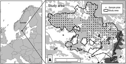
On the Remningstorp estate, 10 m radius sample plots were distributed in a regular grid, resulting in 211 plots. These plots were inventoried in 2010 and 2014 and positioned with a sub-meter accuracy GPS. On each plot, stem diameters for all trees above a diameter threshold of 4 cm were measured and a subsample of these trees was selected and measured for height. Site Index (SI) was assessed from forest floor vegetation and other site characteristics (Hägglund and Lundmark 1977). Models predicting the height of trees from stem diameter were estimated and used for predicting the height of the trees that were not subsampled for height. Height and diameter were then used to calculate stem volume for each tree, according to models by Brandel (1990). Finally, tree-level volumes were aggregated to sample plot totals and recalculated to values per hectare.

This study focused on plots where no, or only light, management actions had been carried out during the four-year study period. Managed (or severely damaged) plots were identified by comparing the measured basal area of each plot in 2010 and 2014. A maximum of 5 m²/ha reduction in the basal area was set as a threshold for a plot to be included in the study. In addition, a few plots with known extreme conditions (species trials with Lodgepole pine, Pinus contorta, otherwise not occurring in southern Swedish forests) were excluded, which left 148 plots for the study. A certain reduction of the basal area was accepted, as natural mortality of trees, sometimes followed by salvage logging, is a normal part of the development of a forest. This was done in analogy to the way that plots were selected for developing growth forecast models (c.f. Appendix to Nyström et al. 2015).

The plots were categorized by dominating tree species, according to the classes used in the growth forecast models: Pine, Spruce, Deciduous, Mixed coniferous, and Mixed coniferous/deciduous. The categories Pine, Spruce, and Deciduous all contain more than 65% of the total growing stock volume of this species. Mixed coniferous stands contain more than 65% coniferous trees but <65% of either spruce or pine. Mixed coniferous/deciduous implies that the deciduous proportion is between 35 and 65%. From Table 1 it can be noted that average volume was larger for plots dominated by coniferous trees than for deciduous trees and that growth was much larger for spruce plots than for the other categories. Spruce was the dominating tree species category in the study area.

Table 1. Mean and standard deviation per species category for the sample plots used in the study, measured in 2010 and 2014.

Species class	n	Age [years] 2010	Volume [m³/ha] measured 2010	SI [m]	Growth [m³/ha]	Volume [m³/ha] measured 2014
			(Mean/standard deviation)
Pine (Scots Pine)	29	85/33.6	212.8/72.2	22.8/4.5	6.5/6.9	238.8/80.3
Spruce (Picea Abies)	76	43/13.9	245.7/153.9	29.6/2.2	17.2/8.8	314.7/174.1
Deciduous^a	26	42.8/24.6	93.9/56.3	29.4/3.1	7.2/5.6	122.8/59
Mixed coniferous^b	6	96.4/44.0	251/45.8	24.0/5.7	11/10.4	295/48.5
Mixed^c	11	55.9/39.3	122.4/80.2	27.4/4.4	5.8/3.8	145.5/79
All plots	148	54.2/30.5	203.7/133.3	27.9/4.2	12.3/9.3	252.7/154

“All plots” refers to the entire set of 148 plots. Site Index (SI) and age were taken from field measurements in 2010. Growth is the difference between growing stock volume measured in 2014 and 2010, respectively, divided by the number of growing seasons (four).

^aThe deciduous class consists of over 65% of the total basal area with deciduous trees, mostly of Birch (Betula SPP), followed by Oak (Quercus Robur).

^bMixed coniferous is a mixture of Pine and Spruce summing to at least 65% of the total basal area.

^cMixed is a mixture of deciduous and coniferous trees where neither category has more than 65% of the total basal area.

For the years between 2010 and 2014, interpolation was used to obtain reference values for growing stock volume, for each plot and year. Linear interpolation was applied, assuming equal amounts of growth each year. Age was also updated one year after each growing season. Growth occurs mainly in spring and early summer in Sweden, and the interpolated yearly growth was added in case the RS data acquisition had occurred later than June 15. We denote the period from June 16 to June 15, the following year, for “state year” to separate it from the calendar year. Apart from volume and age, SI and tree species composition are required for the growth forecasting models used to update predictions in the DA framework. These were taken from the field measurement in 2010, and they were assumed constant throughout the four-year study period.

Remote sensing data

Four types of RS-data from nine acquisitions were utilized in the study: two were ALS, two were DP, three were InSAR and two were OS. The RS-data acquisitions were selected to be roughly equally spread in time and to have properties suitable for predicting growing stock volume. ALS data were used at the start and the end of the study period. This set-up was applied to mimic a realistic scenario in which an initial ALS-based prediction is kept up-to-date through estimates from other, cheaper, sources of RS data in forests where no management has occurred. ALS data were acquired in 2010 and 2014, at approximately the same time as the field inventories were carried out. An important property of ALS data is the season of the year the acquisition was made. If deciduous trees have leaves, growing stock volumes often tend to be overestimated in case no information about tree species is included in the modeling (Bohlin et al. 2017; Nilsson et al. 2017). Both the ALS campaigns were carried out during periods when deciduous trees had their leaves on. Pre-processing of the ALS-point clouds was done using Terrascan (Soininen 2010) and LASTools (Isenburg 2020) to remove flight line overlap and invalid points. Points were then classified into ground and non-ground returns. Non-ground points were normalized to the height above ground level by subtraction from a DEM. Points intersecting the area of each of the sample plots were extracted and plot-level metrics were calculated using FUSION (McGaughey 2014) in a classical area-based approach (Naesset 2002).

The DP data used were three-dimensional (3D) point clouds, mainly representing the upper part of the canopy obtained by matching aerial images taken with stereo overlap. In combination with a high-resolution Digital Elevation Model (DEM), they provide a good source of information to predict forest variables (Bohlin et al. 2012). The variable that is most accurately predicted from DP is height, as density-related metrics from DP are less useful for forest variable prediction compared to density metrics from ALS (Ali-Sisto and Packalen 2017; Bohlin et al. 2017). The Swedish National Land Survey acquires aerial images every second year for southern Sweden and images covering Remningstorp were available from 2012 and 2014 (Lantmäteriet 2019). Pixel size and camera type differed between the two-time points: in 2012 the Z/I camera was used and in 2014 the Vexcel Ultracam, with the ground sampling distances of 0.48 and 0.24 m, respectively. The digital photos were taken with 60% stereo overlap along flight lines and 40% overlap between flight lines. The photos were processed into 3D point clouds using SURE (Rothermel et al. 2012), and the point clouds were height normalized with a DEM with 2 × 2 m grid size from the Swedish National Land Survey (Lantmäteriet 2019). In analogy to the ALS processing into area-based metrics, FUSION was used to process the point clouds into suitable metrics for each sample plot. Details about the DP processing is given in Nyström et al. (2015).

The OS data used in the study were acquired from the SPOT 5 HRG satellite sensor. Images for each year of the study period were provided by the Swedish National Land Survey (Lantmäteriet 2020). SPOT 5 HRG records radiances in the green, red (R), near-infrared ($\mathrm{NIR}$), and shortwave infrared ($\mathrm{SWIR}$) wavelength bands. The ground sampling distance is 10 m for all bands except the SWIR band, which has a 20 m sampling distance; however, for this study, it was resampled to a 10 m distance. In addition to the individual bands, the $\mathrm{NDVI}$ was calculated as $\mathit{NDVI}=(\mathit{NIR}-R)/(\mathit{NIR}+R).$ All pixels intersecting a given sample plot were extracted from the raster images, and OS metrics for the specific plot were calculated as area-weighted means.

Image pairs of TanDEM-X InSAR radar data were used to derive digital surface models (DSMs) by interferometric processing (Moreira et al. 2004; Krieger et al. 2007; Persson and Fransson 2017). Three acquisitions, spread out over the study period, were selected. The main criterion was to select image pairs with a mean height of ambiguity between 35 and 80 m, which is a suitable property for forest variable prediction (Soja and Ulander 2013; Lindgren et al. 2017). The three image pairs were acquired with different polarization properties and during different phenology seasons (see Appendix). The image pairs were processed to derive the interferometric phase height and coherence (Persson and Fransson 2017). The phase height was normalized to the height above ground using the Swedish national ALS-based DEM (Lantmäteriet 2019). The raster data were resampled to 5 × 5 m pixels, and InSAR metrics were derived as weighted averages of pixels overlapping the field plots. For more details, see Lindgren et al. (2017).

Table 2 provides a summary of the RS-data used in this study, presented in chronological order. Additional details about the RS-data can be found in the Appendix.

Table 2. Remote sensing data was used in the study.

Acquisition No. and data type	Acquisition date	Season	Pixel size or point density
1 ALS	2010-08-29	Leaf-on	14.5 points/m²
2 OS	2011-06-06	Leaf-on	10 m
3 InSAR	2012-02-23	Leaf-off	5 m
4 DP	2012-05-23	Leaf-on	7.4 points/m²
5 InSAR	2012-08-28	Leaf-on	5 m
6 OS	2013-07-17	Leaf-on	10 m
7 InSAR	2013-11-18	Leaf-off	5 m
8 DP	2014-07-26	Leaf-on	11.2 points/m²
9 ALS	2014-09-14	Leaf-on	29.6 points/m²

Season refers to if deciduous trees had dropped their leaves or not.

Regression modeling of forest attributes

Plot-level growing stock volumes based on each set of RS data were predicted using regression analysis. The modeling process followed the same methodology for all RS data acquisitions. First, preliminary ordinary least squares models were fitted to the data, assuming a linear relationship between the plot level growing stock volume and the RS metrics. Transformations of independent variables were applied when judged appropriately through studies of residuals plotted versus fitted values and individual RS metrics. Metrics were selected using a forward selection approach, studying AIC for including the appropriate number of explanatory variables into the model. Final models were fitted using the gls function of the nlme-package in R (Pinheiro et al. 2020), with the variance modeled based on the size of the predicted value to account for heteroscedasticity. This procedure was carried out for each of the nine datasets; thus, nine different prediction models were developed.

Error characterization and classical calibration of predictions

The predictions were assessed with regard to their random and systematic errors, conditional on the true biomass on the field plots, applying the following error characterization model (e.g., Tian et al. 2016; Persson and Ståhl 2020) to each dataset: [1] $${\widehat{y}}_{i,t}=A_t+B_t{y}_{i,t}+{ϵ}_{i,t}$$[1]

Here, ${\widehat{y}}_{i,t}$ is the predicted value for plot i at time point t, $y_{i,t}$ is the corresponding field reference (true) value, $A_t$ and $B_t\mathrm{ }$ are model parameters providing insights about the relationship between predicted and true values, and ${ϵ}_{i,t}\mathrm{ }$ is a random error term, assumed to has zero expectation. Based on the field data and the corresponding RS-based predictions, we estimated the parameters of the error characterization model for each of the nine datasets, i.e., [2] $${\widehat{\widehat{y}}}_{i,t}={\widehat{A}}_t+{\widehat{B}}_t{y}_{i,t}$$[2]

The “double hat” notation implies that this model predicts the predicted values from the regression model, based on the true plot volume as a predictor variable. This suggests that the systematic errors can be removed by classical calibration (Osborne 1991) by rearranging (2) so that calibrated predictions are obtained as: [3] $${\widehat{y}}_{i,t,c}=\mathrm{ }\frac{\mathrm{ }({\widehat{y}}_{i,t}-\mathrm{ }{\widehat{A}}_t)}{{\widehat{B}}_t},$$[3] where ${\widehat{y}}_{i,t,c}$ is the calibrated prediction. The calibrated predictions are approximately unbiased throughout the range of predicted values, provided (1) is a valid model. The variances of the calibrated predictions are approximately $\frac{\mathit{var}\left({ϵ}_{i,t}\right)}{B_t^2}$ (1), but note that B must not be zero (or very close to zero) for this variance formula to be applicable. However, in the study, we did not apply this formula directly but estimated the variances empirically based on the residuals obtained from the calibrated predictions. Error characterization and calibration were made specifically for each data acquisition.

Data assimilation

In several previous studies of DA in forestry applications (Ehlers et al. 2013; Nyström et al. 2015; Lindgren et al. 2017), the EKF filter has been applied using the following:

• Initiation: A prediction,$\mathrm{ }{\widehat{y}}_{i,\mathrm{ }t1},$ is obtained from RS-data at the starting time point.

• Updating step: The prediction is updated through a growth model.

• Merging step: Another RS-dataset is acquired and a prediction based on these data is merged with the updated first prediction based on the variances of the two predictions. The variance of the merged prediction is updated accordingly.

• The filter proceeds with another update step, where the updating starts from the merged prediction and its corresponding variance. The cycle of merging and updating steps then continues.

Thus, the first prediction, ${\widehat{y}}_{i,\mathrm{ }t1},$ provides the start for the data assimilation for a given plot i. The application of a growth model provides an updated prediction with at time t2 is: ${\widehat{y}}_{i,\mathrm{ }t2,u}.$ At this time point, a new prediction,$\mathrm{ }{\widehat{y}}_{i,\mathrm{ }t2},$ is prepared from RS data acquired at this time point, and ${\widehat{y}}_{i,\mathrm{ }t2}$ is merged with ${\widehat{y}}_{i,\mathrm{ }t2,u}$ to obtain ${\widehat{y}}_{i,\mathrm{ }t2,\mathrm{ }DA}$ . This is achieved through a weighting procedure: [4] $${\widehat{y}}_{i,t2,DA}=k_{i,t2}{\widehat{y}}_{i,t2,u}+\left(1-k_{i,t2}\right)\mathrm{ }{\widehat{y}}_{i,t2}$$[4]

The weight, k_{i t2}, is chosen so that $\mathit{var}({\widehat{y}}_{i,t2,DA}$) is minimized. In standard EKF, the covariance between the two predictions is assumed to be zero, therefore the weight is calculated as: [5] $$k_{i,t2}=\frac{\mathit{var}\left({\widehat{y}}_{i,t2}\mathrm{ }\right)}{\mathit{var}\left({\widehat{y}}_{i,t2,u}\right)+\mathit{var}\left({\widehat{y}}_{i,t2}\right)},$$[5] and the approximate variance of the merged prediction is: [6] $$\mathit{var}\left({\widehat{y}}_{i,t2,DA}\right)=k_{i,t2}^{2}var\left({\widehat{y}}_{i,t2,u}\right)+{\left(1-k_{i,t2}\right)}^{2}var\left({\widehat{y}}_{i,t2}\right)$$[6]

Here, $\mathit{var}({\widehat{y}}_{i,t2,u})$ is obtained from $\mathit{var}({\widehat{y}}_{i,t1})$ and error propagation through the growth forecast model (described further down). In a third time step, when a prediction,$\mathrm{ }{\widehat{y}}_{i,\mathrm{ }t3},$ from another RS dataset is available, the iteration can proceed by merging this prediction with ${\widehat{y}}_{i,t3,u},$ which is ${\widehat{y}}_{i,t2,DA}$ updated through a growth model. In this study, we used the standard EKF as a reference alternative.

As pointed out in previous studies (Lindgren et al. 2017; Ehlers et al. 2018), the EKF assumption that successive predictions are independent may be a too strong assumption in forestry applications based on RS data. Standard variance minimization technique suggests that a more appropriate weighting formula is: [7] $$k_{i,t2}=\frac{\mathit{var}\left({\widehat{y}}_{i,t2}\right)-\mathit{cov}\left({\widehat{y}}_{i,t2,u,}\mathrm{ }{\widehat{y}}_{i,t2}\right)}{\mathrm{ }\mathit{var}\left({\widehat{y}}_{i,t2,u}\right)+\mathit{var}\left({\widehat{y}}_{i,t2}\right)-2cov\left({\widehat{y}}_{i,t2,u,}\mathrm{ }{\widehat{y}}_{i,t2}\right)\mathrm{ }}$$[7] and the approximate variance after data assimilation is: [8] $$\mathit{var}\left({\widehat{y}}_{i,t2,DA}\right)=k_{i,t2}^{2}var\left({\widehat{y}}_{i,t2,u}\right)+{\left(1-k_{i,t2}\right)}^{2}var\left({\widehat{y}}_{i,t2}\right)+2k_{i,t2}\left(1-k_{i,t2}\right)cov\left({\widehat{y}}_{i,t2,u,}\mathrm{ }{\widehat{y}}_{i,t2}\right)$$[8]

Thus, if the covariance is assumed to be zero, as in standard EKF, the weights applied in the data assimilation step will not be the weights minimizing the variance and the variance estimate for the assimilated prediction will be biased. We thus suggest using a modified version of EKF in this study, based on (7) and (8), which we denote EKFm. The difference between EKF and EKFm is that covariances between predictions are incorporated in the weighting.

In EKFm, the computation of covariance’s requires a recursive algorithm, since the covariance will depend on what “mix” of RS acquisitions is contained in ${\widehat{y}}_{t,u}.$ As a simplification, we assume that the growth forecasts are relatively short and do not change the correlation structure between the predictions involved. The key to determining the covariance between an assimilated prediction and a new prediction after several assimilation steps is to keep track of the composition of the assimilated prediction in terms of acquisition-specific random plot effects. This can be done recursively by, after each assimilation step, computing the composition of the assimilated prediction in terms of what sensors have contributed. For example, an assimilated prediction at time point two (updated to time point three) may contain 60% of acquisition 1 and 40% of acquisition 2. If at time point three, this prediction is combined with a prediction based on acquisition 3, the covariance will be: $$\mathit{cov}\mathrm{ }\left({\widehat{y}}_{t3,u},\mathrm{ }{\widehat{y}}_{t3}\right)=0.6\mathrm{ }\mathit{cov}\mathrm{ }\left({\gamma }_{t1},\mathrm{ }{\gamma }_{t3}\right)+0.4\mathrm{ }\mathit{cov}\mathrm{ }\left({\gamma }_{t2},\mathrm{ }{\gamma }_{t3}\right)$$ In the weighting for this article, the exact variances and covariance of these formulas were replaced by their estimated counterpart.

Growth forecasts and variance propagation

The updating step of DA involves growth forecasting. In this study, the same forecast models as the ones described in the Appendix to Nyström et al. (2015) were used. They followed the form: [9] $$g_{i,t}=\hspace{0.17em}\text{exp}\hspace{0.17em}\left(b_0+{b_1{x}_{i,1,t}+\dots +b}_j{x}_{i,j,t}\right)+e_i$$[9]

Here, g_i,t is the net volume growth over five growth seasons for plot i, with starting conditions corresponding to time point t, and $x_{i,j,t}$ is the jth explanatory variable in the model (for plot i at time point t), b_j is the jth model parameter, and e_i is a random error term, assumed to be normally distributed with zero expectation. The explanatory variables included in the model were the initial plot volume predicted from RS-data, site index (SI), age, and for mixed coniferous forest also the proportion of Norway spruce. Separate models were estimated for different dominating tree species categories, based on their proportion of growing stock volume at the plot according to the classes described in Table 1. We assumed these classes, as well as age and SI, to be known for each plot, based on information from stand registers. An updated prediction was obtained by adding the predicted growth to the predicted volume at the start of the period, i.e.: $${\widehat{y}}_{i,t+1,u}={\widehat{y}}_{i,t}+{\widehat{g}}_{i,t}$$

The variance of ${\widehat{y}}_{i,t,u}$ was approximated through linearization of the growth model around the starting value of the volume, according to the methods in Nyström et al. (2015). To handle unequally long updating periods, the growth predicted according to (9) was adjusted to correspond to the specific length of the updating period.

For small initial volumes (<5 m³/ha) the growth forecasts turned out to be very uncertain. To avoid complications we chose to assign a fixed starting value (5 m³/ha) for the growth function in such cases.

Estimated variances and covariances

The DA procedures require that the variance be estimated for each prediction. For the non-calibrated predictions, we estimated the variances from the residuals emanating from the prediction models being developed specifically for each time point. The standard procedure for estimating residual variance was applied. Whereas we could have estimated variances separately for different subgroups of the plots, we chose not to do so to have a large enough dataset for the variance estimation (the 148 plots). Thus, for a given time point all predictions received the same estimated variance as input to the DA.

For calibrated predictions, a similar procedure was adopted. However, in this case, we used the residuals obtained by comparing calibrated values with field reference values. In this case, the mean value of the residuals was not exactly zero, but close to zero. As for the non-calibrated predictions, all calibrated predictions at a given time-point received the same estimated variance.

Covariances between predictions were estimated for all pairs of time points using the standard formula for empirical covariance estimation. In the case of non-calibrated predictions, we based the covariance estimation on the residuals obtained from the basic predictions models. As for the variances, no grouping of plots was made and thus all plots received the same estimated covariance for a given combination of time points. For calibrated predictions, the residuals entering the empirical covariance estimation were obtained from comparing calibrated predictions with the field references. For purposes of presentation, covariances and variances were also used to compute correlations in the standard way.

Evaluation

To summarize, we compared two different types of volume predictions based on RS data (calibrated and non-calibrated) and for each of them, we evaluated two different data assimilation methods (EKF and EKFm). In addition, we evaluated a case where the initial prediction in the time series (1 ALS) was updated to the end of the study period only through growth forecasts (called forecast from first ALS-prediction). For comparison, all the predictions made at single time points are also presented (called single predictions). A summary of the evaluated prediction types and filter algorithms is presented in Table 3.

Table 3. An overview of the DA methods and prediction methods used in this study, and the cases evaluated when the prediction types and DA methods were combined.

	Calibrated	Non-calibrated
EKF	Case 1	Case 2
EKFm	Case 3	Case 4
Forecast from 1 ALS	Case 5	Case 6
Single predictions	Case 7	Case 8

Evaluations were made at plot level in terms of RMSE and Bias, and rRMSE and rBias, in which cases the RMSE and Bias are expressed in percent of the mean true volume: [10] $$\mathit{RMSE}=\sqrt{\frac{1}{n}\sum _{i=1}^n{r}_{i,t}^2}$$[10] [11] $$\mathit{rRMSE}=\frac{\mathit{RMSE}}{\overline{y}}\mathrm{\hspace{0.17em}}\mathrm{*}\mathrm{\hspace{0.17em}}100$$[11] [12] $$\mathit{Bias}=\frac{1}{n}\sum _{i=1}^n{r}_{i,t}$$[12] [13] $$\mathit{rBias}=\frac{\mathit{Bias}}{\overline{y}}\mathrm{\hspace{0.17em}}\mathrm{*}\mathrm{\hspace{0.17em}}100$$[13]

Where ${\overline{y}}_t=\frac{1}{n}{\sum }_{i=1}^n{y}_{i,t},$ and $r_{i,t}$ being residuals from the specific case evaluated, which can be from any of the cases in Table 3, including the results from assimilation.

We also compared the empirical RMSEs with the theoretical DA variances according to (6) and (8). In the case of applying the latter formulas, an average for all plots was taken, as each plot receives an individual estimated variance through the DA algorithm. [14] $$SD=\sqrt{\frac{1}{n}\sum _{i=1}^n\widehat{\mathit{var}}\left({\widehat{y}}_{i,t,DA}\right)}$$[14] [15] $$\mathit{rSD}=\frac{SD}{\overline{y}}\mathrm{\hspace{0.17em}}\mathrm{*}\mathrm{\hspace{0.17em}}100$$[15]

Results

Results from assimilated predictions

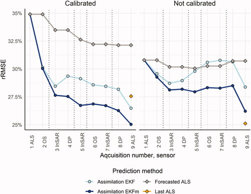
For almost all time points, the EKFm resulted in clearly lower rRMSE than the other methods (Figure 2). This result was valid for both the calibrated and non-calibrated predictions. In the calibrated case, EKFm also reduced the rRMSE compared to using the prediction based on ALS at the final time point. For non-calibrated predictions, EKFm and the final ALS-based prediction had about the same rRMSE. For non-calibrated predictions, the EKF filter led to modest improvements compared to using the initial ALS-based prediction and growth forecasts. EKFm improved the accuracy of predictions, but still the single ALS-based prediction from the final time point was superior to both of the DA-based predictions. However, whereas the general pattern was the same for calibrated predictions the two DA-based methods resulted in substantial decreases of the rRMSE compared to using the initial ALS-based prediction and growth forecasts. Further, both of the DA-based predictions at the final time point were improvements compared to using the ALS-based prediction at this time point. The best accuracy was obtained for EKFm, which reduced the rRMSE from 35% at the initial time point to 25% at the final time point. In contrast to EKF, EKFm also performed consistently better than forecasted ALS in the non-calibrated case. Note that the mean volume was the volume for the particular time point of the acquisition, and since no harvests were performed on the plots the mean volume increased during the study period. Thus, rRMSE had a downward trend, even for forecasted ALS. In absolute values, the RMSE increased over time.

Figure 2. rRMSE, using DA with EKF or EKFm, forecast from first time point (ALS), and ALS for the last time point, for calibrated and non-calibrated predictions. Growth periods are marked with dotted vertical lines.

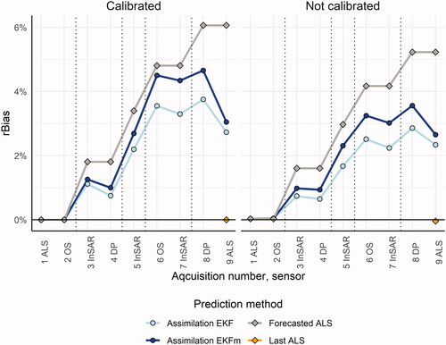
The rBias of predictions increased over time (Figure 3). A positive bias means that the predictions were lower than the average of the field references. The bias increased every time growth was added. The rBias was generally somewhat higher for EKFm compared to EKF.

Figure 3. rBias using DA with EKF or EKFm, forecast from first time point (ALS), and ALS for the last time point, for calibrated and non-calibrated predictions. Growth periods are marked with dotted vertical lines.

Results from single predictions and their error correlation

Table 4 shows the results for the predictions at individual time points, with and without classical calibration. As expected, calibration decreased the accuracy of the individual predictions. The larger the RMSE before calibration, the larger was the increase following calibration. This is due to the central tendency of regression, which was more pronounced when the explanatory power of the data was low.

Table 4. Accuracy for single predictions of growing stock volume, individually assessed by empirical evaluation against the field references.

Acquisition	RMSE (m³/ha)		rRMSE (%)		Bias (m³/ha)		rBias (%)
	Calibrated	Non-calibrated	Calibrated	Non-calibrated	Calibrated	Non-calibrated	Calibrated	Non-calibrated
1 ALS	71	63	34.9	30.8	0	0.06	0	0.03
2 OS	153	100	75.0	49.2	0	0.14	0	0.07
3 InSAR	101	82	46.6	37.9	0	−2.09	0	−0.97
4 DP	89	75	41.4	34.7	0	0.85	0	0.39
5 InSAR	154	105	67.3	45.9	0	−0.35	0	−0.15
6 OS	172	112	71.7	46.7	0	−0.03	0	−0.01
7 InSAR	147	104	61.0	43.3	0	0.46	0	0.19
8 DP	101	84	39.9	33.4	0	0.06	0	0.02
9 ALS	70	63	27.6	25.1	0	−0.11	0	−0.04

The evaluations were made at the time points of the individual acquisitions, with and without classical calibration.

ALS acquisitions led to the most accurate predictions, followed by the DP acquisitions. Both of the ALS acquisitions had an RMSE of 63 m³/ha, but as the mean value of the field references increased due to growth, the rRMSE was lower for the later ALS acquisition (9 ALS). A large variation in terms of accuracy was found among the InSAR acquisitions. This is the sensor where the properties were varying the most (Table 2); the season varies, in contrast to the other sensors which were operated on leaf-on conditions, and the set-up of the system (HOA mainly) varied among the datasets. OS was the least accurate, with very high rRMSEs. Since the estimated models were evaluated on the same sample plots, the bias was close to zero for all predictions. For more details about the RS data and the predictive models, see the Appendix.

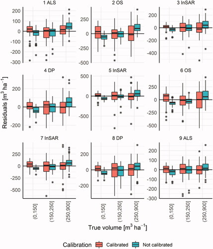
Results from the calibration showed that the tendency to overestimate small true values and underestimate large true values was largely removed by calibration. A boxplot of residuals plotted over categories of true volume is shown in Figure 4. The central line in each box shows the mean value of the residuals (Bias) for the category. When residuals were taken directly from the regression models (non-calibrated), the bias tended to be negative for the lower category and positive for the higher category. The higher the overall residual error, the larger the tendency toward the mean in general, as can be seen when comparing predictions based on OS data with predictions based on ALS data.

Figure 4. Boxplots of residuals for three categories of true volumes on the x-axis. Each group contains roughly the same number of observations.

The correlations between residuals from predictions using different sources of RS data are shown in Figure 5. The left part of the figure shows correlations of residuals after calibration, and the right part the correlations in case no calibration was applied. The removal of the central tendency of regression-based predictions, through calibration, reduced the correlation.

Figure 5. Correlation coefficients of residuals from predictions of growing stock volume using different sources of RS data. The left plot shows residuals after calibration while the right plot shows correlations of residuals for non-calibrated predictions.

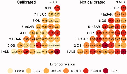
Residuals from predictions based on the same type of RS sensor tended to correlate stronger than residuals from predictions based on different sensors. The lowest correlations were found between OS-predictions and ALS-predictions. Predictions from sensors that capture similar properties of the forest tended to correlate stronger, e.g., DP and ALS. Residuals from predictions based on the two ALS acquisitions correlated very strongly even though four growing seasons separated them. The properties of both ALS acquisitions were similar, e.g., the same season and similar point densities (Table 2). The correlation between the two ALS acquisitions was hardly affected at all by calibration.

Discussion

This study is the first that we are aware of that successfully applies DA on a time series of real RS-data from different sensors for predicting growing stock volume. The results are promising and provide a foundation for the future development of operational methods for keeping forest databases up to date by using data assimilation techniques. With the developed data assimilation methods, accurate predictions from ALS could be maintained and even improved over time, by using more frequent but less accurate remote sensing data. Combined with a method for change detection, this might provide a new paradigm shift where forest databases for management planning are continuously updated rather than being re-made as currently is the case in the Nordic countries.

The assimilations were initiated with predictions from ALS, which is a realistic case in the Nordic countries. To best utilize data from remote sensing sensors that are more frequently available, but less correlated with the growing stock volume, we compensated for the tendency toward the mean due to regression analysis by applying classical calibration, which improved the results. We used the extended Kalman Filter (EKF) in the assimilation step, but with a modification (here called EKFm) that accounted for the error correlations which improved the results greatly (Figure 2).

The two DA-based methods (EKF and EKFm) resulted in notable decreases of the rRMSE compared to using the initial ALS-based prediction and growth forecasts. Further, both of the DA-based predictions at the final time point were improvements over using only the ALS-based prediction at this time point, if the calibration was applied. EKFm outperformed EKF, and unlike EKF in the non-calibrated case, it performed much better than a forecast of 1 ALS (Figure 2).

Even though EKFm accounts for correlated errors, reducing the correlation by applying classical calibration further improved the results. Figure 6 shows empirically evaluated accuracies versus the model-based approximation made in the respective filters (Equations 11[11] $$\mathit{rRMSE}=\frac{\mathit{RMSE}}{\overline{y}}\mathrm{\hspace{0.17em}}\mathrm{*}\mathrm{\hspace{0.17em}}100$$[11] vs. 15[15] $$\mathit{rSD}=\frac{SD}{\overline{y}}\mathrm{\hspace{0.17em}}\mathrm{*}\mathrm{\hspace{0.17em}}100$$[15] ). The discrepancies between model-based and empirical rRMSEs were large for EKF, and ignoring prediction error correlations was making the variance estimates seriously biased, which can be seen for both the calibrated and non-calibrated case where calculated rRMSE (dashed line) differs very much from the empirically evaluated rRMSE (solid line). However, EKFm was a big improvement in this respect. A consequence of using inaccurate prediction error variances in DA is that calculations of Kalman gains (i.e., the weights) will be non-optimal. EKFm thus provides better weights, and also better approximations of the variance of the DA-based predictions. The model-based and empirically evaluated rRMSEs were closer to each other when calibration had been applied, both for EKF and EKFm.

Figure 6. Comparison of empirically evaluated rRMSEs (Equation 11[11] $$\mathit{rRMSE}=\frac{\mathit{RMSE}}{\overline{y}}\mathrm{\hspace{0.17em}}\mathrm{*}\mathrm{\hspace{0.17em}}100$$[11] ) and model-based rRMSEs (Equation 15[15] $$\mathit{rSD}=\frac{SD}{\overline{y}}\mathrm{\hspace{0.17em}}\mathrm{*}\mathrm{\hspace{0.17em}}100$$[15] ) from the filters. Growth periods are marked with dotted vertical lines.

The importance of handling residual error correlations in DA was investigated in Ehlers et al. (2018) and has been confirmed in this study. We addressed correlated errors in three ways: (i) in combining data from several sensors, (ii) through modifying the filter to handle correlations, and (iii) by reducing the error correlations through classical calibration. We also combined these approaches, using calibration and a modified filter to a series of data from different sensors. The developed methods led to results that are superior to those obtained in previous studies, where the EKF filter has been applied together with non-calibrated predictions (Nyström et al. 2015; Lindgren et al. 2017; Ehlers et al. 2018).

Results from the single RS-based predictions showed similar accuracies (Table 4) as those obtained in other studies (Rahlf et al. 2014; Yu et al. 2015; Ehlers et al. 2018). The ALS predictions were at the higher end of previously reported plot level RMSEs, which is probably because of the leaf-on acquisition season (Naesset 2005; Nilsson et al. 2017) in combination with the proportion of broadleaves in the sample plot material (Table 1). Residual plots revealed a pattern of negative bias for deciduous-dominated sample plots, similar to what Nilsson et al. (2017) reported. Assimilation of an OS image after the 1 ALS data largely removed this trend and improved accuracy. In addition, a reason for the high rRMSE, in particular for the 1 ALS acquisition, was also that the mean true volume was lower than in the later part of the time series as the volume increased over the study period.

In most previous studies about DA for forest inventory, a time series of data from a single type of sensor have been used (Nyström et al. 2015; Lindgren et al. 2017). Prediction errors from the same type of sensor tend to be more strongly correlated than prediction errors from different types of sensors (Figures 5) (c.f. Ehlers et al. 2018). Thus, a way to reduce correlations and improve the efficiency of data assimilation may be to use combinations of data from different sensors.

The weakest correlations were obtained between ALS and OS. The frequency of useful OS acquisitions has increased, but it may be questioned if additional OS-based predictions had increased the accuracy of the DA predictions. Ideally, any new prediction should be both accurate and have errors weakly (or negatively) correlated with the errors of the previously assimilated predictions, but the error correlation between the OS-based predictions was large. A richer supply of images provides cloud-free data from early spring (leaf-off) and autumn as well, possibly resulting in lower error correlations. Perhaps the largest benefit of the frequent supply of data lies in the possibility to detect changes, which was not included in this study but should be a part of an operational DA scheme.

All correlation coefficients were lower in the case of calibrated predictions, compared to non-calibrated predictions. This was due to the removal of the tendency toward the mean of the regression-based predictions. However, the more accurate the prediction, the smaller was the effect of calibration on reducing the correlation, as the central tendency is less pronounced for accurate predictions (c.f. Table 4). The linear error characterization model (Equation 1[1] $${\widehat{y}}_{i,t}=A_t+B_t{y}_{i,t}+{ϵ}_{i,t}$$[1] ) might have been too simple in some of the cases it was applied to, since the relation may be nonlinear in the case of saturation effects in RS data. Still, applying classical calibration to the predictions had a notably positive effect on the performance of the EKF and EKFm filters in terms of reducing the empirical rRMSE (Figure 2). Using EKF without calibration led to worse results, for some time points, compared to only making growth forecasts from 1 ALS. When calibrated predictions were used, the rRMSE decreased at almost all time points, and DA provided a more accurate prediction than 9 ALS alone (Figure 2).

The OS-based models had the lowest R² and highest RMSE, and a dramatically increased RMSE if classical calibration were applied. But even though the accuracy of the single OS-based predictions was decreased by calibration, calibration was important when OS-based predictions were part of the DA scheme. Since OS-based predictions were almost uncorrelated with ALS-based predictions, they reduced the rRMSE of the DA prediction substantially when merged with the initial ALS-based prediction (Figure 2); the drop was almost 5% units.

Whereas calibration was applied to the RS-based predictions of volume it was not applied to the growth predictions. Comparing the growth rates (Table 1) with the material used for estimating the growth forecast models (Appendix to Nyström et al. 2015) revealed that the growth rates were comparatively high for the plots in this study. This is a likely reason for the bias presented in Figure 3, which increased each time a growth forecast had been made but remained more or less constant when new predictions were assimilated without a previous growth forecast. Thus, a natural extension of this study would be to calibrate not only the RS-based predictions but also the growth forecasts.

We used Taylor linearization to propagate the variance through the non-linear growth forecast model. This method works best if the model is close to being linear. Our models were of an exponential form (Equation 9[9] $$g_{i,t}=\hspace{0.17em}\text{exp}\hspace{0.17em}\left(b_0+{b_1{x}_{i,1,t}+\dots +b}_j{x}_{i,j,t}\right)+e_i$$[9] ) and thus far from being linear. Problems with the Taylor linearization were experienced for low volumes, which made the approximated variances very uncertain for such cases. Better methods to handle non-linear forecast models could thus be an area for future developments, for example through using Bayesian methods (Ehlers et al. 2013). Another development area could be the recursive handling of covariances. The algorithm we used required taking all pairs of RS-data in the time series into account, which leads to somewhat tedious computations. Further, we did not handle covariance propagation due to the growth model. A computational benefit of the EKF filter is that covariances between predictions can be ignored and thus predictions in the past can be disregarded when the updated DA prediction is merged with a new prediction. Over a limited number of time steps, it is straightforward to handle covariances in the way it was done in this study, but it becomes increasingly difficult as the number of time steps increases. It is likely that an operational EKFm scheme should disregard historic predictions and make use of only a certain number of latest predictions, at least when computing covariances.

This study has shown that DA has the potential to improve the accuracy of a model of the forest state over time by continuously assimilating predictions from various RS sensors. In an operational DA framework, additional functionalities would be needed in addition to the core functionalities explored here. Examples are RS-based routines for change detection (Kennedy et al. 2010; Grabska et al. 2020), prediction of SI (Noordermeer 2020), and tree species (Persson et al. 2018). Another important issue is the cost-effective supply of reference data for the estimations. For this to be realistic, automatic collection of stem data from harvesters (Holmgren et al. 2012), back-pack scanners, and cell phones (Liang et al. 2018), as well as cooperation between forest organizations might be needed. Also, practical use of DA would require aggregation to larger units, such as forest stands (c.f. evaluation in Nyström et al. 2015). This would pose additional challenges, as the error correlation between spatially adjacent plots would need to be estimated.

Acknowledgments

The authors would like to thank Benoît Gozé for translating the title and abstract to French.

Disclosure statement

The authors declare no conflicts of interest.

Additional information

Funding

This work was supported by the Swedish Research Council FORMAS, grant number 942-2015.

Appendix

Details about the remote sensing data

 

Table A.1. Details about the ALS data.

Acquisition number	Acquisition date	Scanner	Flying altitude (m)	Point density (points/m²)
1 ALS	2010-08-29	TopEye s/N 700	400	14.5
9 ALS	2014-09-14	Riegl LMS Q680i	300	29.6

Table A.2. Details about the DP data.

Acquisition number	Acquisition date	Camera	Flying altitude (m)	Ground sampling distance (m)
4 DP	2012-05-23	Zeis/Integraph DMC	4,800	0.48
8 DP	2014-07-26	Vexcel UltraCamX	2,800	0.24

Table A.3. Details about the TanDEM-X InSAR data.

Acquisition number	Acquisition date	Orbit	Polarization	HOA
3 InSAR	2012-03-23	146	VV	79
5 InSAR	2012-08-28	146	VV	37
7 InSAR	2013-11-18	78	HH	72

Table A.4. Details about the OS data.

Acquisition number	Acquisition date	Satellite and sensor	Path/row	Ground sampling distance (m)
2 OS	2013-07-17	SPOT 5 HRG	053/231	10–20
6 OS	2011-06-06	SPOT 5 HRG	053/231	10–20

 

Estimated predictive modelsTable A.5. Coefficients and included variables for the estimated models predicting forest growing stock volume.

Acquisition number	Acquisition date	Variable	Coefficient	SE
1 ALS	2010-08-29	Intercept	2.4	7.29
		MeanH^2	1.5	0.199
		VR*P95	0.07	0.016
2 OS	2011-06-06	Intercept	520	83.4
		B4^2	1,400,000	239,000
		NDVI	−520	79.2
		B1/B4	−450	89.8
3 InSAR	2012-02-23	Intercept	46	8.94
		ISH^2	0.89	0.0566
4 DP	2012-05-23	Intercept	77	9.14
		CUBEmean^3	0.032	0.00323
		P95/CV	0.24	0.112
5 InSAR	2012-08-28	Intercept	33	17.3
		(ISH + 10)^2	0.35	0.0319
6 OS	2013-07-17	Intercept	790	126
		B4^2	4,800,000	723,000
		NDVI	−630	104
		B1/B4	−1,100	199
7 InSAR	2013-11-18	Intercept	350	69.2
		(ISH + 5)^2	0.6	0.074
		COH	−350	84.7
8 DP	2014-07-26	Intercept	70	10.5
		CUBEmean^3	0.034	0.00242
		VR/CV	0.035	0.0132
9 ALS	2014-09-14	Intercept	30	6.09
		MeanH^2	1.4	0.215
		VR*P95^2	4.1e-05	9.1e-06

Point cloud metrics abbreviated by: MeanH: mean of points heights above ground; VR: vegetation ratio; P95: height percentile 95; CUBEmean: cube-root of the mean of heights to the cube; CV: coefficient of variation.

References

- Ali-Sisto, D., and Packalen, P. 2017. “Forest change detection by using point clouds from dense image matching together with a LiDAR-derived terrain model.” IEEE Journal of Selected Topics in Applied Earth Observations and Remote Sensing, Vol. 10(No. 3): 1197–1206. doi:https://doi.org/10.1109/JSTARS.2016.2615099.
- Ayrey, E., and Hayes, D.J. 2018. “The use of three-dimensional convolutional neural networks to interpret LiDAR for forest inventory.” Remote Sensing, Vol. 10(No. 4): 649. doi:https://doi.org/10.3390/rs10040649.
- Bohlin, J., Bohlin, I., Jonzén, J., and Nilsson, M. 2017. “Mapping forest attributes using data from stereophotogrammetry of aerial images and field data from the national forest inventory.” Silva Fennica, Vol. 51(No. 2): 2021. doi:https://doi.org/10.14214/sf.2021.
- Bohlin, J., Wallerman, J., and Fransson, J.E.S. 2012. “Forest variable estimation using photogrammetric matching of digital aerial images in combination with a high-resolution DEM.” Scandinavian Journal of Forest Research, Vol. 27(No. 7): 692–699. doi:https://doi.org/10.1080/02827581.2012.686625.
- Brandel, G. 1990. Volymfunktioner för enskilda träd: tall, gran och björk, Report 26. Garpenberg: Department of Forest Production, Swedish University of Agricultural Sciences.
- Chirici, G., Giannetti, F., McRoberts, R.E., Travaglini, D., Pecchi, M., Maselli, F., Chiesi, M., and Corona, P. 2020. “Wall-to-Wall spatial prediction of growing stock volume based on Italian National Forest Inventory plots and remotely sensed data.” International Journal of Applied Earth Observation and Geoinformation, Vol. 84: 101959. doi:https://doi.org/10.1016/j.jag.2019.101959.
- Ehlers, S., Grafström, A., Nyström, K., Olsson, H., and Ståhl, G. 2013. “Data assimilation in stand-level forest inventories.” Canadian Journal of Forest Research, Vol. 43(No. 12): 1104–1113. doi:https://doi.org/10.3390/rs10050667.
- Ehlers, S., Saarela, S., Lindgren, N., Lindberg, E., Nyström, M., Persson, H.J., Olsson, H., and Ståhl, G. 2018. “Assessing error correlations in remote sensing-based estimates of forest attributes for improved composite estimation.” Remote Sensing, Vol. 10(No. 5): 667. doi:https://doi.org/10.3390/rs10050667.
- Grabska, E., Hawryło, P., and Socha, J. 2020. “Continuous detection of small-scale changes in Scots Pine dominated stands using dense Sentinel-2 time series.” Remote Sensing, Vol. 12(No. 8): 1298. doi:https://doi.org/10.3390/rs12081298.
- Hägglund, B., and Lundmark, J.-E. 1977. Site Index Estimation by Means of Site Properties of Scots Pine and Norway Spruce in Sweden. Studia Forestalia Suecica. Issue: 138. Stockholm: Swedish College of Forestry.
- Holmgren, J., Barth, A., Larsson, H., and Olsson, H. 2012. “Prediction of stem attributes by combining airborne laser scanning and measurements from harvesters.” Silva Fennica, Vol. 46(No. 2): 227–239. doi:https://doi.org/10.14214/sf.56.
- Isenburg, M. 2020. “LAStools.” Internet, assessed Oct 7, 2020. https://rapidlasso.com/lastools/.
- Kalman, R.E. 1960. “A new approach to linear filtering and prediction problems.” Journal of Basic Engineering, Vol. 82(No. 1): 35–45. doi:https://doi.org/10.1115/1.3662552.
- Kalman, R.E., and Bucy, R.S. 1961. “New results in linear filtering and prediction theory.” Journal of Basic Engineering, Vol. 83(No. 1): 95–108. doi:https://doi.org/10.1115/1.3658902.
- Kangas, A., Astrup, R., Breidenbach, J., Fridman, J., Gobakken, T., Korhonen, K.T., Maltamo, M., Nilsson, M., Nord-Larsen, T., Næsset, E., and Olsson, H. 2018. “Remote sensing and forest inventories in Nordic countries – roadmap for the future.” Scandinavian Journal of Forest Research, Vol. 33(No. 4): 397–412. doi:https://doi.org/10.1080/02827581.2017.1416666.
- Kennedy, R.E., Yang, Z., and Cohen, W.B. 2010. “Detecting trends in forest disturbance and recovery using yearly Landsat time series: 1. LandTrendr — Temporal segmentation algorithms.” Remote Sensing of Environment, Vol. 114(No. 12): 2897–2910. doi:https://doi.org/10.1016/j.rse.2010.07.008.
- Koivuniemi, J., and Korhonen, K. T. 2009. ” Inventory by compartments.” In Forest Inventory – Methodology and Applications, edited by A. Kangas and M. Maltamo. New York, NY: Springer.
- Krieger, G., Moreira, A., Fiedler, H., Hajnsek, I., Werner, M., Younis, M., and Zink, M. 2007. “TanDEM-X: A satellite formation for high-resolution SAR interferometry.” IEEE Transactions on Geoscience and Remote Sensing, Vol. 45(No. 11): 3317–3341. doi:https://doi.org/10.1109/TGRS.2007.900693.
- Krutchkoff, R.G. 1967. “Classical and inverse regression methods of calibration.” Technometrics, Vol. 9(No. 3): 425–439. doi:https://doi.org/10.1080/00401706.1967.10490486.
- Lantmäteriet 2019. “Geodata products.” Internet, accessed Feb 6, 2020. https://www.lantmateriet.se/en/maps-and-geographic-information/geodataprodukter/produktlista/.
- Lantmäteriet 2020. “SACCESS.” Internet, accessed Nov 24, 2020. https://saccess.lantmateriet.se/portal/saccess_se.htm.
- Liang, X., Kukko, A., Hyyppä, J., Lehtomäki, M., Pyörälä, J., Yu, X., Kaartinen, H., Jaakkola, A., and Wang, Y. 2018. “In-situ measurements from mobile platforms: An emerging approach to address the old challenges associated with forest inventories.” ISPRS Journal of Photogrammetry and Remote Sensing, Vol. 143: 97–107. doi:https://doi.org/10.1016/j.isprsjprs.2018.04.019.
- Lindgren, N., Persson, H.J., Nyström, M., Nyström, K., Grafström, A., Muszta, A., Willén, E., Fransson, J.E.S., Ståhl, G., and Olsson, H. 2017. “Improved prediction of forest variables using data assimilation of interferometric synthetic aperture radar data.” Canadian Journal of Remote Sensing, Vol. 43(No. 4): 374–383. doi:https://doi.org/10.1080/07038992.2017.1356220.
- McGaughey, R. J. 2014. “FUSION–Providing fast, efficient, and flexible access to LIDAR, IFSAR, and terrain datasets.” Internet. http://forsys.cfr.washington.edu/fusion/fusionlatest.html.
- Moreira, A., Krieger, G., Hajnsek, I., Hounam, D., Werner, M., Riegger, S., and Settelmeyer, E. 2004. “TanDEM-X: A TerraSAR-X add-on satellite for single-pass SAR interferometry.” Paper presented at IGARSS 2004: IEEE International Geoscience and Remote Sensing Symposium: Science for Society: Exploring and Managing a Changing Planet. Anchorage, AK: IEEE Proceedings, Vol 1–7: 1000–1003.
- Naesset, E. 2005. “Assessing sensor effects and effects of leaf-off and leaf-on canopy conditions on biophysical stand properties derived from small-footprint airborne laser data.” Remote Sensing of Environment, Vol. 98(No. 2–3): 356–370. doi:https://doi.org/10.1016/j.rse.2005.07.012.
- Naesset, E. 2002. “Predicting forest stand characteristics with airborne scanning laser using a practical two-stage procedure and field data.” Remote Sensing of Environment, Vol. 80(No. 1): 88–99. doi:https://doi.org/10.1016/S0034-4257(01)00290-5.
- Naesset, E., Gobakken, T., Holmgren, J., Hyyppä, H., Hyyppä, J., Maltamo, M., Nilsson, M., Olsson, H., Persson, Å., and Söderman, U. 2004. ” “Laser scanning of forest resources: The Nordic experience.” Scandinavian Journal of Forest Research, Vol. 19(No. 6): 482–499. doi:https://doi.org/10.1080/02827580410019553.
- Nilsson, M., Nordkvist, K., Jonzén, J., Lindgren, N., Axensten, P., Wallerman, J., Egberth, M., et al. 2017. “A nationwide forest attribute map of Sweden predicted using airborne laser scanning data and field data from the National Forest Inventory.” Remote Sensing of Environment, Vol. 194: 447–454. doi:https://doi.org/10.1016/j.rse.2016.10.022.
- Noordermeer, L. 2020. Large-area forest productivity estimation using bitemporal data from airborne laser scanning and digital aerial photogrammetry. PhD Thesis number 2020:37. Ås: Norwegian University of Life Sciences.
- Nyström, M., Lindgren, N., Wallerman, J., Grafström, A., Muszta, A., Nyström, K., Bohlin, J., et al. 2015. “Data assimilation in forest inventory: First empirical results.” Forests, Vol. 6(No. 12): 4540–4557. doi:https://doi.org/10.3390/f6124384.
- Osborne, C. 1991. “Statistical calibration: A review.” International Statistical Review , Vol. 59(No. 3): 309–336. doi:https://doi.org/10.2307/1403690.
- Persson, H.J., and Fransson, J.E.S. 2017. “ “Comparison between TanDEM-X and ALS based estimation of above ground biomass and tree height in boreal forests.” Scandinavian Journal of Forest Research, Vol. 32(No. 4): 306–314. doi:https://doi.org/10.1080/02827581.2016.1220618.
- Persson, H.J., and Ståhl, G. 2020. “Characterizing uncertainty in forest remote sensing studies.” Remote Sensing, Vol. 12(No. 3): 505. doi:https://doi.org/10.3390/rs12030505.
- Persson, M., Lindberg, E., and Reese, H. 2018. “Tree species classification with multi-temporal Sentinel-2 data.” Remote Sensing, Vol. 10(No. 11): 1794. doi:https://doi.org/10.3390/rs10111794.
- Pinheiro, J., Bates, D., DebRoy, S., and Sarkar, D. R. 2020. “nlme: Linear and Nonlinear Mixed Effects Models.” R Core Team. Internet. https://cran.r-project.org/package=nlme.
- Rabier, F. 2005. “Overview of global data assimilation developments in numerical weather-prediction centres.” Quarterly Journal of the Royal Meteorological Society, Vol. 131(No. 613): 3215–3233. doi:https://doi.org/10.1256/qj.05.129.
- Rahlf, J., Breidenbach, J., Solberg, S., Naesset, E., and Astrup, R. 2014. ” “Comparison of four types of 3D data for timber volume estimation.” Remote Sensing of Environment, Vol. 155(No. Special issue): 325–333. doi:https://doi.org/10.3390/f6114059.
- Reese, H., Nilsson, M., Pahén, T.G., Hagner, O., Joyce, S., Tingelöf, U., Egberth, M., and Olsson, H. 2003. “Countrywide estimates of forest variables using satellite data and field data from the National Forest Inventory.” Ambio, Vol. 32(No. 8): 542–548. doi:https://doi.org/10.1579/0044-7447-32.8.542.
- Rothermel, M., Wenzel, K., Fritsch, D., and Haala, N. 2012. “SURE: Photogrammetric Surface Reconstruction from Imagery.” Paper presented at LC3D Workshop. Berlin, 4–5 December 2012.
- Soininen, A. 2010. “TerraScan User’s Guide.” Espoo: TerraSolid Ltd.
- Soja, M. J., and Ulander, L. M. H. 2013. ” Digital canopy model estimation from TanDEM-X interferometry using high-resolution lidar DEM.” Paper presented at International Geoscience and Remote Sensing Symposium (IGARSS). Melbourne, July 2013.
- Stewart, L.M., Dance, S.L., and Nichols, N.K. 2008. “Correlated observation errors in data assimilation.” International Journal for Numerical Methods in Fluids, Vol. 56(No. 8): 1521–1527. doi:https://doi.org/10.1002/fld.1636.
- Tian, Y., Nearing, G.S., Peters-Lidard, C.D., Harrison, K.W., and Tang, L. 2016. “Performance metrics, error modeling, and uncertainty quantification.” Monthly Weather Review, Vol. 144(No. 2): 607–613. doi:https://doi.org/10.1175/MWR-D-15-0087.1.
- Wallerman, J., and Holmgren, J. 2007. “Estimating field-plot data of forest stands using airborne laser scanning and SPOT HRG data.” Remote Sensing of Environment, Vol. 110(No. 4): 501–508. doi:https://doi.org/10.1016/j.rse.2007.02.028.
- Weiskittel, A. R., Hann, D. W., Kershaw, J. A., and Vanclay, J. K. 2011. Forest growth and yield modeling. Hoboken, NJ: Wiley.
- Weisberg, S. 2014. Applied linear regression. Hoboken, NJ: Wiley.
- Yu, X., Hyyppä, J., Karjalainen, M., Nurminen, K., Karila, K., Vastaranta, M., Kankare, V., et al. 2015. “Comparison of laser and stereo optical, SAR and InSAR point clouds from air- and space-borne sources in the retrieval of forest inventory attributes.” Remote Sensing, Vol. 7(No. 12): 15933–15954. doi:https://doi.org/10.3390/rs71215809.