Monitoring Crops Using Compact Polarimetry and the RADARSAT Constellation Mission

Abstract

The RADARSAT Constellation Mission (RCM) can acquire imagery in Compact Polarimetric (CP) mode. With this new mode, and the increased revisit with three satellites, RCM can contribute to operational crop monitoring at national scales. The four Stokes (S₀, S₁, S₂ and S₃) and three m-chi decomposition (surface, double bounce, volume) parameters were used to identify crops (pasture/forage, barley, wheat, canola, flaxseed, peas, lentils) with a Random Forest classifier. The Stokes and m-chi parameters delivered maps of similar accuracies (95% overall accuracy) and were only slightly less accurate than a classification using optical satellite imagery (97%). To understand why Stokes parameters worked well in classifying crops, scattering responses for wheat, canola, lentils and peas were plotted on the Poincaré sphere. These responses were interpreted in the context of the degree of polarization and were related to crop phenology. These plots revealed that early and late in the season the polarized component of the scattered wave remained circular. However, in the active season when crop structure was changing, scattered waves became more elliptically polarized. Although the amount of polarized scattering was lower mid-season, the change in ellipticity was helpful in separating crop types.

RÉSUMÉ

La mission de la Constellation RADARSAT (MCR) peut acquérir des images en mode polarimétrique compact (CP). Grâce à ce nouveau mode et à la revisite accrue avec trois satellites, RCM peut contribuer à la surveillance opérationnelle des cultures à l’échelle nationale. Les quatre paramètres de Stokes (S0, S1, S2 et S3) et trois paramètres de décomposition m-chi (surface, double rebond, volume) ont été utilisés pour identifier les cultures (pâturage/fourrage, orge, blé, canola, graines de lin, pois, lentilles) à l’aide d’un classificateur Random Forest. Les paramètres de Stokes et de m-chi ont fourni des cartes d’une précision similaire (précision globale de 95%) et elles n’étaient que légèrement moins précises qu’une classification utilisant l’imagerie satellitaire optique (97%). Pour comprendre pourquoi les paramètres de Stokes fonctionnaient bien dans la classification des cultures, des réponses de la diffusion pour le blé, le canola, les lentilles et les pois ont été tracées sur la sphère de Poincaré. Ces réponses ont été interprétées dans le contexte du degré de polarisation et étaient liées à la phénologie des cultures. Ces tracés ont révélé qu’au début et à la fin de la saison, la composante polarisée de l’onde diffusée restait circulaire. Cependant, pendant la saison active, lorsque la structure des cultures changeait, les ondes diffusées devenaient polarisées plus elliptiquement. Bien que la quantité de la diffusion polarisée ait été plus faible à la mi-saison, le changement d’ellipticité a été utile pour séparer les types de cultures.

Introduction

The RADARSAT constellation mission

In 2019 Canada launched the RADARSAT Constellation Mission (RCM), a government-owned and operated constellation and a follow-on to the highly successful RADARSAT-1 and RADARSAT-2 missions. The primary driver of RCM is to support Government of Canada operational activities for maritime surveillance, ecosystem monitoring and disaster management. The RCM design offers a number of advantages to previous RADARSAT missions. These mission enhancements were deemed of high importance to fulfill government operations. With a three-satellite constellation, RCM significantly improves upon the 24-day revisit of RADARSAT-2. Each RCM satellite has a 12-day revisit, and when all satellites are used together, exact revisit improves to 4 days. Beam steering increases re-look at any point on the Earth. RCM can provide daily coverage of Canada’s territorial and adjacent waters (Doyon et al. 2018) with multiple daily re-looks possible at higher latitudes. Spatial resolutions vary depending on beam mode, but range from nominally 3–100 m.

RCM retains a fully polarimetric (FP) mode on each satellite. As implemented on RADARSAT-2 and RCM, the FP mode transmits and receives two orthogonal polarizations (horizontal (H) and vertical (V)), and retains phase. These orthogonal polarizations must be interleaved during transmission, which requires that the pulse repetition frequency (PRF) be twice that required of single or dual-polarized SARs (Charbonneau et al. 2010). With doubling the PRF, the FP swath width must be reduced by half (Charbonneau et al. 2010). On RCM for example, the swath width of FP acquisitions is nominally 20 km. Although the full scattering matrix offers a rich dataset, the small FP swath is not practical for national-scale operational mapping.

During the design of RCM, Compact Polarimetry (CP) was proposed as a partial solution for users who require wide swath coverage but want to retain polarization richness (Raney 2007). The potential of CP had been demonstrated in radar astronomy (Raney et al. 2021). This prompted government scientists to evaluate simulated CP data and the research confirmed that the CP solution described by (Raney 2007) could deliver products of value to government operations, including accurate crop inventories (Charbonneau et al. 2010). CP is implemented on RCM as a right-handed circular (RHC) transmit with H + V polarizations recorded coherently on return (circular-transmit and linear-receive or CL). A circular transmit waveform is created when the H and V feeds are driven simultaneously but out of phase by 90° (Raney 2007). With only a single transmit polarization (RHC), power requirements are reduced compared to FP modes. CP can be selected for most RCM modes, including wide swath modes (as an example, Low Resolution 100 m mode (500 km swath)) and higher resolution modes (as an example, Spotlight (20 km swath)).

The scattering information in CP modes is presented in a 2 × 2 covariance matrix rather than the 3 × 3 covariance matrix associated with FP products (Raney 2007). Although the higher dimensionality of FP provides more information about target scattering than CP, early results using CP simulated from RADARSAT-2 found that CP data delivered crop classifications with higher accuracies when compared to single and dual linearly polarized SAR (Charbonneau et al. 2010, McNairn and Shang 2016). Information derived from CP can be broadly grouped into backscatter intensities, the four Stokes parameters, parameters derived from Stokes, and scattering power decompositions.

The stokes parameters and CP decomposition

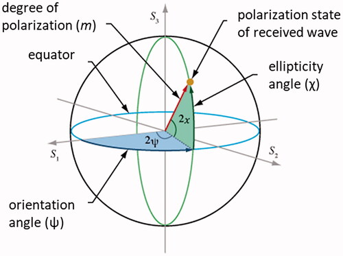
The Stokes parameters describe the polarization state of a partially polarized electromagnetic (EM) field (Raney et al. 2021). Scattering from most distributed targets, such as vegetation, is typically partially polarized given the multiple scattering events that take place within this complex target. The first Stokes parameter (S₀) indicates the total intensity of the radar backscatter (polarized and unpolarized), which is the sum of the powers of the two orthogonally-polarized received waves. The other three parameters (S₁, S₂, and S₃) describe the properties of the polarized portion of the EM field. S₁ describes the preponderance of linear horizontal polarized light over linear vertical polarized light, S₂ describes the preponderance of linear +45° polarized light over linear −45° polarized light and S₃ describes the preponderance of right-handed circular polarized light over left-handed circular polarized light (Collett 2005). S₁ was determined from the difference between the powers of the receive channels. S₂ and S₃ are derived from complex cross-products of the received EM waves (Raney 2006, 2019). When viewed in the direction of propagation the electric field vector rotates and (generally) traces the shape of an ellipse. Linear and circular polarized propagations are considered special cases of elliptically polarized waves. The angle of ellipticity (χ) falls within the range from −45° to +45° (circular ±45°; linear 0°; elliptical all other angles). The inclination angle (orientation (ψ) angle) falls between −180° and +180°.

The Stokes parameters S₁, S₂, and S₃ can also be expressed in terms of the Poincaré variables, where χ indicates ellipticity, ψ is the orientation of the long axis of polarization ellipse and m is the degree of polarization (DoP) defined by (Raney et al. 2012) as: (1) $$\text{degree of polarization }\left(m\right)=\mathrm{ }\frac{\sqrt{{\mathrm{S}}_1^2+\mathrm{ }{\mathrm{S}}_{2\mathrm{ }}^2{+\mathrm{ }\mathrm{S}}_{3\mathrm{ }}^2}}{{\mathrm{S}}_0}.$$(1)

The Poincaré sphere (Figure 1) is one approach to visualize the polarized portion of a partially polarized wave, and to interpret the state of the received wave with respect to Stokes parameters S₁, S₂ and S₃, as well as the ellipticity and orientation angles. The length of a vector from the core to the surface of the Poincaré sphere represents the DoP (m). If the scattered wave is fully polarized (m = 1), the polarization state value of a wave will map onto the surface of the sphere. Scattering from vegetation is expected to have at least some component of the response unpolarized and as such, the polarization state will lie beneath the surface of the sphere. Circularly polarized waves are mapped at the north and south poles of the Poincaré sphere and linearly polarized waves at the equator. All other wave configurations (with at least some ellipticity) will fall in the other regions of the sphere.

Figure 1. Schematic of Poincaré sphere (adapted from https://www.thorlabschina.cn/newgrouppage9.cfm?objectgroup_id=142)00).

Both coherent and incoherent approaches to decomposition have been developed and applied to fully polarimetric SAR for a range of applications. Incoherent methods are most often applied to targets with distributed scatterers, as is the case with vegetation cover. The Cloude–Pottier eigen-based decomposition extracts a set of feature parameters to characterize scattering from the target in terms of the randomness of the scatterer (entropy), dominant type of scattering mechanism (alpha angle) and the relative power of the second and third eigenvectors (anisotropy) (Cloude and Pottier 1996, McNairn et al. 2009). Cloude et al. (2012) adapted the eigen-based decomposition to estimate entropy and alpha from compact polarimetry data. Model-based decompositions separate the total power received into scattering mechanisms. These mechanisms include single-bounce (surface) scattering, double-bounce (dihedral) scattering and multiple (volume) scattering (Freeman and Durden 1998). The Pseudo-3 decomposition is derived by relating the 3 component model of the FP covariance matrix transformed to a coherency matrix, expressing scattering as volume, double and surface scattering based upon the Stokes parameters (Wang et al. 2015).

Raney et al. (2012) introduced the m-chi (m-χ) decomposition for single-transmitted dual-receive polarization data, as is the case with CP (RHC transmit, H + V receive). This decomposition utilizes the Poincaré variable χ, S₀, and DoP (m). The DoP is the single most important parameter characteristic of a partially polarized EM field and (1-m) is closely related to entropy (Raney 2007). For the second component of this decomposition, the Poincaré ellipticity parameter χ was selected as it is one of the three principal components (m, χ, ψ) needed to describe the polarized portion of a partially polarized wave (Raney 2007). The sign of χ indicates the presence of even versus odd bounce scattering, including when the transmitted EM field is not perfectly circularly polarized.

The m-chi decomposition allocates total received power into one of three sources of scattering: (2) $$R^{2\mathrm{ }}\left(\mathit{double}\mathrm{ }\mathit{bounce}\right)=\mathrm{ }m{\mathrm{S}}_0\mathrm{ }(1+\hspace{0.17em}\mathit{\text{sin}}\hspace{0.17em}2\chi )/2$$(2) (3) $$G^{2\mathrm{ }}\left(\mathit{volume}\mathrm{ }\mathit{scattering}\right)=\mathrm{ }{\mathrm{S}}_0\mathrm{ }(1-m)$$(3) (4) $$B^{2\mathrm{ }}\left(\mathit{single}\mathrm{ }\mathit{bounce}\right)=\mathrm{ }m{\mathrm{S}}_0\mathrm{ }(1-\hspace{0.17em}\mathit{\text{sin}}\hspace{0.17em}2\chi )/2$$(4)

The m-delta decomposition has also been applied to CP data, and is derived from the Stokes child parameters of m, circular ratio, relative phase (δ) and χ (Raney 2006, Brisco et al. 2013). However, delta (δ) is also dependent on the orientation of the polarization ellipse of the backscattered EM field (Raney et al. 2012). The implication, as explained in Raney et al. 2012, is that if there is a significant linearly polarized component in the transmitted field (due to an imperfect circularly polarized transmit wave) then a change in the angular orientation of any dihedral structure in the scene could cause the sign of delta to reverse polarity. In contrast, the m-chi decomposition has proven to be robust in the event that the transmitted field is not perfectly circularly polarized. In addition to this advantage, the m-chi decomposition is directly interpretable relative to the Stokes parameters. New and adapted decompositions for both FP and CP data continue to be developed. This study focuses on the m-chi decomposition given its availability for operational implementation with RCM and the promising results with m-chi as reported in other published studies (De et al. 2014; Uppala et al. 2016; Chirakkal et al. 2017; Dasari and Lokam 2018; Mahdianpari et al. 2019). Nevertheless, future research to assess additional decomposition methods for mapping and monitoring cropland would be of significant interest.

Review of CP research for crop classification

With limited access to CP data, much of the published research has simulated compact polarimetric data from fully polarimetric modes, with many studies using FP data acquired by RADARSAT-2 to complete this simulation. Charbonneau et al. (2010) performed an early assessment of the performance of CP for crop classification. In this research, four RADARSAT-2 FP images were acquired over an eastern Canadian test site and used to simulate CP data. The cropping mix at this site included corn, soybeans, wheat and pasture-forage. Using the Stokes parameters derived from the four simulated CP images, a Decision Tree (DT) classifier delivered an end-of-season crop classification accuracy of 91%. This end-of-season map accuracy was similar to that produced using dual-polarizations (HH + VV and HH + HV) and the Freeman-Durden decomposition parameters. However, Stokes parameters from CP provided the highest overall accuracy for early season crop acreage estimation, and increased early season mapping accuracies for individual crops.

The DT classifier is implemented by Agriculture and Agri-Food Canada (AAFC) in their Annual Crop Inventory (ACI), which has produced crop maps for more than a decade (Davidson et al. 2017). Despite 10 years of operations using a DT approach, a Random Forest (RF) classifier is being considered in the next generation of operations given its improved performance relative to DTs (Deschamps et al. 2012). Dingle Robertson et al. (2019) applied an RF classifier to simulated CP data acquired in a western Canadian research site, with a more complex cropping mix compared to the site considered by Charbonneau et al. (2010). Three RADARSAT-2 images were used in the simulation and ten CP features and decompositions were generated for each image and included in a data stack for classification. Preliminary overall accuracies were poor (<65%) although accuracies for some crops (canola and soybeans) were higher (71–78%). The poor results may have been due to a limited temporal coverage (only 3 images for the entire season). Mahdianpari et al. (2019) achieved higher accuracies using simulated CP over this Canadian test site with four RADARSAT-2 images, and with a focus on mid-season (mid-July) classification. Applying a RF classifier to map forage, oats, wheat, corn, canola and soybeans, overall accuracies of 88.23% (FP) and 82.12% (CP) were reported. These were an improvement over a dual-polarization (HH + HV or VV + VH) classification (77.35% overall accuracy). The variable importance analysis determined that for both FP and CP, the volumetric component of the decomposition features and the right-circular transmit and right-circular receive (RR) and HV backscatter intensities contributed most to the classification. In the case of CP both the m-delta and m-chi decompositions were applied, although Mahdianpari et al. (2019) demonstrated that these two decompositions were highly correlated.

Brisco et al. (2013) simulated a CP dataset from four RADARSAT-2 images acquired over a test site in China, to evaluate the accuracy of CP for rice classification. Using a Support Vector Machine (SVM) classifier, the Stokes parameters and m-delta (m-δ) decomposition mapped rice at comparable accuracies (95–96% overall accuracy). These researchers concluded that classification accuracy increases as polarization diversity increases. Although CP did not perform as well as FP data, CP did outperform dual polarizations. The majority of CP analysis has been based upon C-band data, however, Xie et al. (2015) compared land cover classification results between FP and simulated CP from TerraSAR-X. This comparison was applied to a site in China with the main land cover including rice, banana, sugarcane, eucalyptus, water and built-up areas. Similar to results by Brisco et al. (2013), classification accuracies were slightly higher for X-band FP (95%) relative to simulated CP (91%). Ballester-Berman and Lopez-Sanchez (2012) examined the correlation between three hybrid-polarity parameters (degree of polarization, relative phase and the circular polarization ratio) simulated from L-band data, and measures of crop development (LAI, biomass, height, crop cover and phenological stage). Wet biomass was correlated with relative phase (winter wheat and maize) and the circular polarization ratio (maize) while height of winter rape was correlated with the degree of polarization.

In 2012, the Indian Space Research Organization (ISRO) launched the Radar Imaging Satellite 1 or RISAT-1, a C-band SAR which carries a scientific CP mode. Other satellites such as Japanese Aerospace Exploration Agency (JAXA)’s ALOS-2 PalSAR-2 and Comisión Nacional de Actividades Espaciales (Conae)’s SAOCOM sensors also carry experimental CP modes. As a comparison to RCM, the RISAT-1 Fine Resolution Mode (FRS) transmits a right circularly polarized wave and receives a backscattered signal in two orthogonal polarizations (H and V) (Chirakkal et al. 2017). Research using RISAT-1 CP mode provided a first look at the performance of real CP data for crop classifications. De et al. (2014) reported that the m-χ decomposition coupled with a supervised Wishart classification was suitable for classifying crops such as banana, cotton and rice, with overall accuracies between 81% and 87% depending on the date used. Chirakkal et al. (2017) applied the two hybrid polarimetric decomposition techniques, m-δ and m-χ, to CP images from RISAT-1 acquired over a site in India, with a mix of rice, cotton, pulses, wheat, mustard, chickpeas, and pea crops. After applying a maximum likelihood classification, these researchers reported that the m-χ decomposition resulted in better crop separability. Dave et al. (2017) evaluated the sensitivity of CP data from RISAT to the growth of cotton crops in India. In addition to the Stokes parameters, these authors generated the degree of polarization, alpha, entropy, anisotropy, RVI, RH and RV intensities, and applied several decompositions (m-delta, Freeman-2 and 3 component, van Zyl) from the C-band satellite data. This study found that RH and RV intensities were correlated with the height, age and biomass of cotton. The volume component of all decomposition was sensitive to plant height, age and biomass. RVI increased with the age of the cotton plants.

Studies have also evaluated CP against other sources including dual-pol RISAT-1 data and data from optical satellites. Using an SVM classifier and a single RISAT-1 image, Dasari and Lokam (2018) concluded that CP data delivered a 92.3% overall accuracy compared to a 76.8% accuracy using dual-pol data to separate urban, water, vegetation and bare soil land covers. They also reported that the m-χ decomposition is more robust than other decompositions when the transmitted waveform is not perfectly circularly polarized. Uppala et al. (2016) tested RISAT-1 data for identifying maize fields and investigated the performance of CP decomposition parameters (degree of circularity, relative phase, DoP, double bounce, odd bounce, and volume bounce) using a parallelepiped minimum distance classifier. Results were compared to accuracies produced from optical Resourcesat-2 LISS-III data. Overall classification results showed that the m-χ decomposition provided accurate information from a single-date RISAT-1 image, with producers and users accuracies for maize recorded as 90.63% and 87.88%, respectively.

Research objectives

The primary objective of this research is to assess CP data acquired by RCM for the enhancement of crop inventory operations. AAFC has been classifying the agriculture extent of Canada on an operational basis since 2009 and includes SAR data in the classification when optical images are unavailable due to cloud cover. The SAR data ingested in the ACI operations have typically included 2 or 3 dual polarization vertical send, vertical receive (VV) and vertical send, horizontal receive (VH) RADARSAT-2 images from the beginning, middle and end of the growing season. The ACI uses as many cloud-free optical images (or portions of images) as are available throughout the growing season. Optical bands used in the classifier are the blue, red, green, near infrared (NIR) and two short wave infrared (SWIRs) bands from (historically) Landsat satellites, and more recently, the Sentinel-2 satellites. The reliance on optical data poses operational challenges. Cloud cover impedes the collection of optical imagery and masking of clouds can be taxing on operational resources.

The outcome of the analysis with RCM CP data is impactful for not only Canadian operations, but for other regional and national agricultural monitoring activities. In this study, classification is performed using the four Stokes parameters and m-chi decomposition parameters derived from a temporal stack of RCM CP images and compares the performance of CP to the existing operations which require inputs of optical imagery.

A secondary science objective is to develop an understanding of the Stokes parameters with respect to crop biophysical characteristics. Although these SAR parameters have been used in classifications, their interpretation relative to developing crop canopies is not fully understood. As such, this research also assesses the temporal characteristics of the CP-derived polarized components of the Stokes parameters by plotting RCM scattering responses on the Poincaré sphere and comparing these to field observations of the phenology of four crops: canola, wheat, lentils and peas.

Methods

Site description

The area of interest known as “Kenaston,” is located in Saskatchewan, Canada (Figure 2). This site is south of the provincial capital city, Saskatoon, and west of the town of Kenaston (Figure 2b). Saskatchewan (Figure 2c) is one of Canada’s three Prairie Provinces, and is an important agricultural production region of the country. In 2020, the value of agri-food exports from Saskatchewan was valued at $16.9 billion (CDN) (Saskatchewan Ministry of Agriculture, Annual Report for 2020–2021 n.d.).

Figure 2. (a) Agriculture extent of Canada as mapped by AAFC since 2009, (b) location of Kenaston within the province of Saskatchewan and (c) RCM multi-temporal composite of the Kenaston study site.

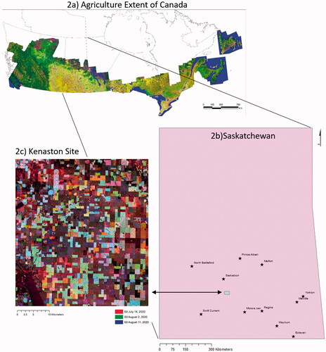
Kenaston has been an important site of agricultural remote sensing research in Canada and was the location of the Canadian Experiment for Soil Moisture in 2010 (CanEx-SM10), a calibration and validation research experiment which supported both the Soil Moisture and Ocean Salinity (SMOS) and the Soil Moisture Active and Passive (SMAP) missions (Magagi et al. 2013). Production in this region is dominated by annual cropping of lentils and other pulses, cereals such as wheat, oat and barley, canola and other oilseeds, as well as acreages of forage and pasture lands. This prairie region is typically arid to sub-humid with a cold climate and occasional summer rains (Shook et al. 2013) These climatic conditions drive some producers to rely on pivot irrigation. In general, the area is flat with slopes of less than 2% and minimal runoff. There are countless small wetlands, also known as sloughs or prairie potholes which act as internal drainage throughout the region (Shook et al. 2013; Tetlock et al. 2019).

Field data collection

Starting June 11th (2020) and for each week thereafter until September 7th, crop phenology was recorded for 12 fields each of four different crop types (canola, wheat, lentils and peas). Phenology was indicated according to the Biologische Bundesanstalt, Bundessortenamt, and Chemical (BBCH) scale (Meier 2001; BBCH Growth Stages: Lentils were developed based upon Peas growth stages from Meier 2001). BBCH describes crop growth using two digits, with a high level categorization of growth stage indicated from 0 to 9 (Table 1). The second digit of the BBCH designation adds precision and indicates the percentage of the canopy which has reached the growth stage. For example, 67 indicates that the crop has entered flowering and that 70% of the canopy has flowered. Weekly BBCH observations included collection of a GPS coordinate of the observation point and photograph of the field. Through the 2020 season, 48 fields (12 fields × 4 crop types) were visited 16 times, leading to a total of 768 observations of growth stage.

Table 1. BBCH phenology categories.

BBCH primary category	Growth stage description
	Canola	Wheat	Peas/Lentils
00	Germination	Germination	Germination
10	Leaf development	Leaf development	Leaf development
20	Formation of side shoots	Tillering
30	Stem elongation	Stem elongation	Stem elongation
40		Booting
50	Inflorescence emergence	Inflorescence emergence, heading	Inflorescence emergence
60	Flowering	Flowering	Flowering
70	Development of fruit	Development of fruit	Development of fruit
80	Ripening	Ripening	Ripening
90	Senescence	Senescence	Senescence

Classification validation and training data were acquired following typical windshield survey methodologies (Waldner et al. 2016) where the crop grown in each field is noted from the roadside, and the observation includes a GPS coordinate. These point observations were subsequently assigned to quarter section polygons (ISC.ca) and field polygons were buffered inward by 100 m to avoid erroneous contributions from edges, ditches and roads, etc. In total 1247 crop type observations were collected from mid to late August 2020, and these included 17 different crop types. During the field data quality control review, minor crops with less than 25 observations were removed from the dataset resulting in a final reference set of 1187 observations. The seven crop classes retained included pasture/forage, barley, wheat, canola, flaxseed, peas and lentils. These data were then split using a stratified sampling randomizer with approximately 65–70% fields assigned to training and 30–35% fields assigned to validation data. Stratified sampling takes into consideration differences between groups (e.g., classes), particularly class size, as opposed to random sampling which treats groups as equal with an equal probability of being sampled. This ensures that the classes have proportional and representative samples, and that small classes are not over sampled nor large class under sampled. The ratio of the split depended on the spatial distribution and number of fields per crop type. A summary of the number of field samples used in the classifier is provided in Table 2. Total pixel counts per crop type for training and validation data were made once the field data were rasterized.

Table 2. Numbers of ground observations per crop type.

	Fields		Pixels
	Training	Validation	Training	Validation
Pasture/Forage	40	22	7247	4014
Barley	42	20	7658	3657
Wheat	41	27	7453	4912
Canola	383	158	69607	28709
Flaxseed	17	8	3106	1447
Peas	67	32	12131	5701
Lentils	220	110	39956	19885

SAR data description and processing

RCM data were programmed over the Kenaston site by tasking all three RCM satellites (RCM1, RCM2 and RCM3). The images were acquired in ScanSAR Compact Polarization (CP) mode with imagery delivered as Single Look Complex (SLC) data. This mode has a nominal spatial resolution of 30 m and an overall image swath of 125 km. A full ScanSAR image is composed of four sub-swaths with multiple bursts, and are available in RCM beams A, B, C and D. The difference between these modes are their incidence angle. RCM beams A and D still require calibration (Touzi et al. 2021), therefore both B and C beams were utilized for the crop classification objective. Incident angles for ScanSAR B (23.68°–32.73° from near to far range) are slightly less than angles for C (30.62°–38.31°). The interpretation of the Stokes parameters with respect to crop type and stage of phenology used only RCM CP beam B. Limiting this particular analysis to beam B avoided mixing changes in scattering due to crop development with changes due to variations in incident angles. In total, 17 RCM images were acquired for the 2020 growing season (Table 3).

Table 3. RCM image acquisition dates. All dates were used for crop classification.

	RCM1 30mCP B mode	RCM2 30mCP B mode	RCM2 30mCP C mode	RCM3 30mCP B mode	RCM3 30mCP C mode
June	12*, 24*	16*	9		1
July		10*, 14*, 26		6*, 18*, 30*	1
August	27*	7*	2, 31	11*

Dates indicated with * were used in the interpretation of Stokes parameters with respect to crop phenology.

All SAR images were pre-processed according to the methodologies as described in (Dingle Robertson et al. 2020a, 2020b) using the Earth Observation Data Management System (EODMS) SAR Toolbox (Natural Resources Canada, Canada Center for Mapping and Earth Observation 2020). The order of operations to generate the Stokes parameters and m-chi decomposition parameters from RCM SLC data is as follows: application of a polarimetric speckle filter, generation of polarimetric parameters, and terrain correction of the generated products. Prior to the generation of the SAR polarimetric parameters including the Stokes parameters and the m-chi decomposition parameters, a 5 × 5 (for phenology assessment) and 9 × 9 (for classification) polarimetric boxcar speckle filter was applied to the SLC data. Filtering is necessary to reduce the noise inherent in SAR data and in general, larger kernels improve classification outcomes (Dingle Robertson et al. 2020a). Previous research has found that with increasing kernel size, overall classification results improve until a maximum is achieved at which point the overall classification accuracy begins to decline (Dingle Robertson et al. 2020a). The Kenaston site is dominated by large fields and similar to what was found in Dingle Robertson et al. (2020a), a larger 9 × 9 kernel can be accommodated to reduce noise and improve field classifications. Crop growth, measured by biomass and phenology, can vary across a field due primarily to variations in soil properties. Given this potential spatial variation in crop growth, a smaller kernel was selected for analysis of phenology impacts on Stokes parameters. The polarimetric boxcar filter calculates the value of a pixel based upon the average value of a sliding window. In the case of polarimetric data the calculation considers the estimated covariance matrix (Bouchemakh et al. 2008, Sun et al. 2016). The boxcar filter preserves the phase information which is imperative when deriving polarimetric parameters, in this case the Stokes parameters (S₀, S₁, S₂ and S₃) and the m-chi decomposition (volume, surface, double bounce scattering contributions).

The expression of the Stokes vector for CP is generated from a 2 × 2 matrix and described as follows (Raney et al. 2012; Raney et al. 2021): (5) $${\mathrm{S}}_0=〈{\left|E_{RH}\right|}^2+ {\left|E_{RV}\right|}^2〉$$(5) (6) $${\mathrm{S}}_1=〈{\left|E_{RH}\right|}^2-\mathrm{ }{\left|E_{RV}\right|}^2〉=\mathrm{ }m{S}_o\mathrm{ }\hspace{0.17em}\mathit{\text{cos}}\hspace{0.17em}2\chi \mathrm{ }\hspace{0.17em}\mathit{\text{cos}}\hspace{0.17em}2\psi$$(6) (7) $${\mathrm{S}}_2=2\mathrm{ }Re\mathrm{ }〈E_{RH}{E}_{RV}^{\mathrm{*}}〉=\mathrm{ }m{S}_o\mathrm{ }\hspace{0.17em}\mathit{\text{cos}}\hspace{0.17em}2\chi \mathrm{ }\hspace{0.17em}\mathit{\text{sin}}\hspace{0.17em}2\psi$$(7) (8) $${\mathrm{S}}_3=2\mathrm{ }Im\mathrm{ }〈E_{RH}{E}_{RV}^{\mathrm{*}}〉=\mathrm{ }m{S}_o\hspace{0.17em}\mathit{\text{sin}}\hspace{0.17em}2\chi$$(8) where $\left|E\right|$ is the amplitude of the electric field, superscript ∗ denotes the complex conjugate, and 〈⋯〉 denotes the spatial average over a moving window. Re represents the real and Im the imaginary value of the complex cross-product amplitude. When viewed in the direction of propagation the electric field vector rotates and (generally) traces the shape of an ellipse. Linear and circular polarized propagations are considered special cases of elliptically polarized waves. The angle of ellipticity ($\chi )$ falls within the range from −45° to +45° (circular ±45°; linear 0°; elliptical all other angles). The inclination angle (orientation $(\psi$) angle) falls between −180° and +180°.

For the intensity channels of RH (right-circular transmit, horizontal received) and RV (right-circular transmit, vertical receive) noise was reduced separately and only using a Gamma Maximum A Posteriori (MAP) filter. An adaptive filter, the Gamma MAP filter assumes a Gamma distribution of speckle noise that is typical for agriculture and has been tested and utilized for AAFC’s ACI for over 10 years (Davidson et al. 2017; Dingle Robertson et al. 2020a; Gagnon and Jouan 1997).

Following noise reduction, the Stokes parameters, m-chi decomposition parameters and the intensity channels were all terrain corrected. Terrain correction, or ortho-rectification, corrects the image by removing the effects of angle and terrain and projects the image into a known coordinate system. All SAR image products were terrain corrected using a rational function model. The rational function model relates ground points to image satellite points using Rational Polynomial Coefficients (RPCs). RPCs generally have no physical meaning, are expressed as a polynomial fraction and are provided by the satellite metadata (Hu et al. 2004). Rational function terrain correction has been in use since the early 2000s and has been adopted by the EODMS SAR toolbox as the method of choice for ortho-rectification. Following ortho-rectification, SAR products were included in different classification data stacks, with the training field data, to test combinations of SAR parameters for crop classification.

Crop classification method

AAFC ACI operations use a See 5.0 (Quinlan 1990) Decision Tree (DT) classifier, a method also used by the United States Department of Agriculture (USDA) for their annual Cropland Data Layer (CDL) (Boryan et al. 2011). The classification workflow was developed and customized by AAFC (McNairn, et al. 2009; Shang et al. 2009; Fisette et al. 2015; Davidson et al. 2017) and using this DT methodology overall classification accuracies for Saskatchewan have ranged from 80% in 2009 to 94% in 2020 (Agriculture and Agri-Food Canada 2020). Despite the operational reliance on a DT classifier, assessments of a Random Forest (RF) classifier have consistently delivered improved overall and individual class accuracies (Deschamps et al. 2012; Dingle Robertson et al. 2020b). RF is a non-parametric classifier and an ensemble method in which many decision trees are grown, resulting in a “forest”. Training data (e.g., field observations) and predictive variables (e.g., satellite data) are subset repeatedly and individual trees are grown. Each tree terminates in end node classes. Using each tree’s end node class as a vote, a final classification is made. Classes that have the majority of votes from all the trees become the class assigned in the final product (Breiman 2001). The objective of this research is to measure the performance of RCM for crop classification rather than to deliver a comparative analysis of different classification algorithms. As such, considering the results from the previously cited research (e.g., Deschamps et al. 2012; Fisette et al. 2015; Dingle Robertson et al. 2020b, etc.) and the goal to support and improve national operations, an RF was applied to the RCM data acquired over the Kenaston site. An RF also produces a measure of variable importance with respect to input data layers (Deschamps et al. 2012; Millard and Richardson 2015; Dingle Robertson et al. 2019; Mahdianpari et al. 2019). Variable importance is calculated by first taking the number of votes for correct classes in the out-of-bag data and calculating this for each tree. Next, random shuffling of the predictor’s values (e.g., satellite data) is completed and the new correct number of votes is assessed. The new correct number of votes is subtracted from the original correct number of votes and an average is taken for all the trees in the forest. This score is normalized by the standard deviation. Variables with large values are ranked as more important (Breiman 2001). Variable importance is used to determine the contribution of different satellite data layers (date of acquisition and SAR parameter) to the classification outcome. Many channels of data can be synthesized from polarimetric SAR data and volumes of data can increase significantly when considering multiple acquisitions through the growing season. Rating the importance of input channels helps to reduce data volumes, remove redundant inputs and eliminate data that confuse classification outcomes.

The input parameters selected for the RF classification method were set as 150 trees and 10 variables (the number of predictive variables (e.g., earth observation data) to evaluate when splitting each node) as previous studies have shown that altering the number of trees and the number of variable parameters had minimal effects on the overall classification accuracies (Deschamps et al. 2012; Dingle Robertson et al. 2019). Several different combinations of the CP parameters were assessed and classified. The parameters included in the classification are listed in Table 4. These combinations included: all CP parameters together (intensity, Stokes parameters, and m-chi decomposition parameters); Stokes and m-chi parameters together; each parameter set separately; and the parameters of m-chi volume scattering, S₀ alone and S₁, S₂, and S₃. These combinations of data were assessed to help inform the operational inclusion of the CP parameters and led to eight different classification runs. Accuracies were assessed using an error matrix comparing validation data with classification outputs. Overall accuracy and the kappa coefficient were generated for each data set, and user and producer accuracies were generated for individual crop types.

Table 4. List of parameters included in the classification runs.

Parameter	Definition
Stokes 0	$S_0=〈{\left|E_{RH}\right|}^2+ {\left|E_{RV}\right|}^2〉$
Stokes 1	$S_1=〈{\left|E_{RH}\right|}^2- {\left|E_{RV}\right|}^2〉$ $= m{S}_o \hspace{0.17em}\mathit{\text{cos}}\hspace{0.17em}2\chi \hspace{0.17em}\mathit{\text{cos}}\hspace{0.17em}2\psi$
Stokes 2	$S_2=2\mathit{\text{ Re }}〈E_{RH}{E}_{RV}^{*}〉= m{S}_o \hspace{0.17em}\mathit{\text{cos}}\hspace{0.17em}2\chi \hspace{0.17em}\mathit{\text{sin}}\hspace{0.17em}2\psi$
Stokes 3	$S_3=2\mathit{\text{ Im }}〈E_{RH}{E}_{RV}^{*}〉= m{S}_o\hspace{0.17em}\mathit{\text{sin}}\hspace{0.17em}2\chi$
m-Chi double bounce	$R^{2 }= m{S}_0 (1+\hspace{0.17em}\mathit{\text{sin}}\hspace{0.17em}2\chi )/2$
m-Chi volume scattering	$G^{2 }= S_0 (1-m)$
m-Chi single bounce	$B^{2 }= m{S}_0 (1-\hspace{0.17em}\mathit{\text{sin}}\hspace{0.17em}2\chi )/2$
RH	Intensity
RV	Intensity

Creation of Poincaré plots and calculation of DoP

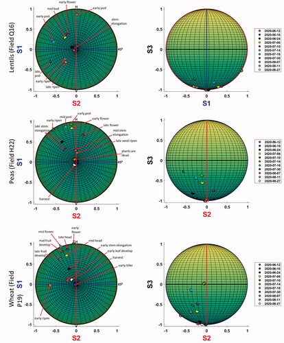
The RF classification sorts the importance of individual data channels for crop identification. However, interpretation of the biophysical drivers of SAR response is helpful to understand the selection of these parameters by the ensemble of forests that comprise the RF. To aid in this analysis, the polarized components of the Stokes parameters (S₁, S₂ and S₃) were plotted on the Poincaré sphere. The S₁, S₂ and S₃ parameters were normalized so that points fell on the surface of the sphere. For visual clarity, the Poincaré spheres were utilized in this work (Figures 5 and 6) to analyze only the evolution of the polarized component of the signal over the measurement period. Each data point consisting of S₁, S₂, and S₃ components was treated as 3-D vectors. Each of these vectors was normalized into unit vectors, which have a length of 1, thus falling on the surface of a unit sphere. Most scattering responses were plotted on the Left Handed Circular (LHC) projection of the Poincaré sphere, which displays scattering using S₁ and S₂ axes. This projection also provides information on S₃, with points closer to the origin of the projection having higher values of S₃. The exception was canola where handedness changed from left to right during some BBCH stages, and a Right Hand Circular (RHC) projection was also required. Only the RCM images acquired in beam B were used in this analysis (see Table 3) to eliminate the impact of incident angle differences. This provided 11 RCM repeat passes of beam B from 12 June until 27 August. Weekly phenology observations within two days of these RCM dates were used to label and interpret how the polarization ellipse changed as crops developed.

Another important response parameter to consider is the DoP (m) given that the 3 D Poincaré plots consider only the polarized scattering component. Microwaves transmitted from SAR antennas are completely polarized. For data acquired in CP mode, RCM transmits a wave in which the tip of the electric field vector rotates during propagation, tracing the shape of a circle. However, once this right handed circular wave interacts with a target, the DoP can change. With completely unpolarized energy, the plane of propagation and thus the polarization of the scattered wave changes randomly. Partial depolarization of incident waves can occur in vegetation canopies which create opportunities for multiple scattering events. For large dense canopies with complex structures composed of stems, leaves, flowers and fruit which are oriented in many different directions, the direction of polarization of the scattered wave can vary significantly from point to point within the field and within a SAR resolution cell. As a result, it is expected that as crops grow and the canopy structure increases in complexity, the DoP will decrease. In this analysis, DoP was calculated from the Stokes parameters using Equation 1(1) $$\text{degree of polarization }\left(m\right)=\mathrm{ }\frac{\sqrt{{\mathrm{S}}_1^2+\mathrm{ }{\mathrm{S}}_{2\mathrm{ }}^2{+\mathrm{ }\mathrm{S}}_{3\mathrm{ }}^2}}{{\mathrm{S}}_0}.$$(1) . Changes in DoP were plotted and interpreted with respect to crop phenology.

Results and discussion

Crop classification

Table 5 outlines the accuracy results obtained for each of the eight SAR classification runs, in declining order of overall accuracy (from left to right in the table). As a point of reference, the table also includes the accuracy results obtained in the same region using the ACI DT methodology with post-processing filtering applied. During 2020 the classification of this region was limited to optical satellite data only and included as inputs to the classifier, five cloud-free Landsat 8 (August 15 and August 31) and Sentinel-2 (June 1, July 11 and July 24) images.

Table 5. 2020 RCM data classifications in overall accuracy descending order.

	ACI		Stokes & M-chi CP Parameters		All M-chi		RH, RV, Stokes & M-chi CP Parameters		All Stokes Parameters
	UA	PA	UA	PA	UA	PA	UA	PA	UA	PA
Pasture/ Forage	97.96	90.00	91.48	86.31	89.59	87.18	92.41	87.40	94.13	83.23
Barley	92.88	92.49	94.36	91.81	93.10	91.01	96.74	86.48	96.02	88.24
Wheat	95.57	91.47	89.84	84.49	89.57	81.75	85.97	82.39	84.90	82.51
Canola	99.00	99.93	96.27	99.65	96.00	99.62	96.32	99.66	96.75	99.58
Flaxseed	88.49	74.91	98.77	49.97	98.66	50.26	89.33	40.80	96.29	41.86
Peas	97.29	96.49	99.16	87.83	98.77	87.30	99.46	88.28	99.03	87.90
Lentils	96.37	98.74	93.67	98.27	93.56	97.84	92.84	98.64	91.58	98.56
Overall Accuracy	97.26		94.91		94.55		94.50		94.29
Kappa Coefficient	0.96		0.93		0.92		0.92		0.92
	M-chi Volume Only		RH,RV		S1, S2 and S3		S0 Only
	UA	PA	UA	PA	UA	PA	UA	PA
Pasture/ Forage	82.44	83.54	93.18	79.23	93.31	79.55	89.53	78.03
	89.31	84.34	95.35	84.60	90.69	79.50	95.54	73.55
Barley	86.61	73.30	78.15	74.93	80.96	73.18	77.73	68.36
Wheat	95.90	99.56	95.89	99.15	94.70	99.33	96.48	99.49
Canola	78.58	41.04	82.09	27.87	88.42	34.19	61.42	18.53
Flaxseed	98.31	86.61	98.22	82.35	84.80	80.94	98.77	87.16
Peas	90.73	96.09	88.44	97.86	90.79	96.55	85.29	97.02
Lentils	92.59	92.17	91.50	91.14	93.56	97.84	92.84	98.64
Overall Accuracy	0.90		0.89		0.88		0.87
Kappa Coefficient	0.96		0.93		0.92		0.92

Overall accuracies, Kappa coefficients, users’ accuracies (UA) and producers’ accuracies (PA) are provided.

The SAR data combination with the highest overall accuracy was the classification run which included input of all four Stokes and all three m-chi decomposition parameters. Using these seven CP parameters, the overall classification accuracy was 94.9%, an accuracy slightly lower than that achieved using only optical satellite data with post-processing filtering (97.3%). In all cases except for the flaxseed and barley classes, the optically based classification provided higher user’s and producer’s accuracies for all individual crop types. For the flaxseed class, the optical data achieved a significantly lower user’s accuracy at 88.5% as compared to that achieved using the SAR parameters (98.8%). For the barley class, the optical data achieved a slightly lower user’s accuracy of 92.9% as compared to the SAR parameters (94.4%). However, an optical classification of flaxseed and barley (74.9% and 92.5% respectively) outperformed a SAR classification (50.0% and 91.8% respectively) when only producer’s accuracies are considered. Flaxseed accuracies were significantly lower relative to all other classes. It is likely that this lower accuracy is due to the more limited training data (17 fields) for this class because of the lower acreages of flaxseed in this region.

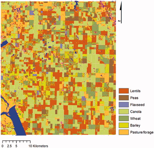
With the exception of flaxseed, all other individual classes achieved an accuracy of 85% or above, meeting the accuracy target set by the Canadian operations (Davidson et al. 2017). Figure 3 is a classification map created using the Stokes and m-chi parameters.

Figure 3. Classified map of the Kenaston study site using a Random Forest classifier and inputs of the four Stokes and three m-chi parameters generated using RCM CP images. 17 30mCP images were used to create this figure.

Regardless of the combination of SAR parameters included in the RF, the overall accuracies were all above 90%. Although differences in overall accuracy varied by only approximately 5% among the classification runs, some observations are noteworthy. Outcomes using either the three m-chi or four Stokes parameters were similar and combining these seven parameters did not significantly increase overall accuracy. This is unsurprising considering that the m-chi decomposition parameters are derived from Stokes parameters (Equations 2–4).

Accuracies using only intensity (RH + RV or S₀) were two of the lowest among the classification runs. As well, the addition of the RH, RV intensities to the run which included all 4 Stokes and all 3 m-chi parameters did not improve overall or individual class accuracies. When assessing just the Stokes parameter classification combinations overall accuracies reached 94.3% when all four Stokes parameters were used, compared to 91.14% when using only S₀ and 91.5% when using S₁, S₂, and S₃ together. As such, the use of all four Stokes parameters assisted in improving overall classification outcomes. However, at the crop level, some crops had higher user’s accuracies with inputs of only S₁, S₂, S₃ (pasture/forage, wheat, flaxseed and lentils) in contrast to higher user’s accuracies when only S₀ was used (barley, canola and peas). The crop classes that had higher producer’s accuracies for the S₁, S₂, S₃ classification run, compared to the S₀ classification, were pasture/forage, barley, wheat, and flaxseed. S₀ had higher producer’s accuracies for canola, peas and lentils. The importance of the first Stokes parameter in identifying some crops, and the remaining three parameters for classifying other crops, explains the advantage of including all four Stokes parameters to achieve a higher overall accuracy.

Table 6 shows the order of importance of contributing SAR parameters (S₀, S₁, S₂, S₃) per date and for each class type, for the classification run that used all Stokes parameters. This comparison assists in determining the importance of each of the four Stokes parameters to classification of individual crops and thus, overall classification outcomes. For peas, S₀ was important in identifying this crop and ranked as the most important input for the July 6 RCM image followed by rankings of 3rd, 4th and 6th for July 18, August 2, and June 1, respectively. This finding is reflective of the higher user’s and producer’s accuracies for peas when only S₀ was used as input to the RF classifier, compared against a classification limited to S₁, S₂, S₃ and excluding S₀. Interestingly, the importance of the total intensity (S₀) was less for the other crop types. Of note for canola, S₀ did not rank within the top ten importance contributions. For most other crops, S₀ was ranked in the top 10 importance variables only once or twice. For wheat, total intensity for the June 1 RCM image was ranked 10th; for lentils 4th (August 2) and 8th (July 6th). Finally, S₀ was not ranked within the top ten for the overall classification. This underscores why the intensity-based classifications (RH, RV and S₀) were on the lower end of the overall classification accuracies, and resulted in more individual classes with user’s and producer’s accuracies less than 85%. As such, S₁, S₂ and S₃ inputs were important contributors to a successful classification.

Table 6. Order of importance ranking from Random Forest classification.

	Crop types
	Pasture/Forage	Barley	Wheat	Canola	Flaxseed	Peas	Lentils	Overall
1	S0	S1	S1	S1	S0	S0	S3	S1
	Jun 1	Jul 26	Jul 26	Jul 14	Jun 1	Jul 6	Aug 2	Jul 1
2	S1	S2	S2	S2	S3	S2	S3	S2
	Jun 16	Jun 1	Jun 1	Jul 1	Jun 1	Jun 16	Aug 27	Jul 1
3	S2	S1	S2	S2	S1	S0	S3	S2
	Jun 1	Jul 14	Jun 16	Jun 9	Jul 26	Jul 18	Jun 1	Jun 9
4	S2	S3	S3	S1	S3	S0	S0	S3
	Jun 9	Aug 2	Aug 2	Jul 6	Aug 2	Aug 2	Aug 2	Jun 1
5	S2	S2	S3	S1	S2	S1	S3	S2
	Jul 1	Jun 9	Jul 30	Jul 1	Jun 9	Jul 1	Aug 31	Aug 31
6	S3	S2	S2	S2	S2	S0	S1	S1
	Aug 27	Aug 11	Jul 1	Aug 31	Jun 16	Jun 1	Jul 26	Jul 14
7	S1	S0	S3	S1	S2	S2	S1	S2
	Aug 31	Jun 1	Aug 27	Aug 2	Aug 11	Jul 1	Jul 14	Jun 1
8	S3	S3	S3	S2	S1	S3	S0	S1
	Aug 31	Jul 30	Jun 1	Jun 16	Jun 16	Jul 1	Jul 6	Jun 16
9	S2	S2	S1	S2	S2	S2	S3	S3
	Aug 11	Jun 16	Jul 14	Aug 27	Jul 1	Jun 1	Jul 30	Aug 27
10	S1	S0	S0	S3	S3	S1	S1	S3
	Jun 9	Jul 6	Jun 1	Jul 30	Jun 9	Jul 6	Jul 6	Aug 2

Contributing bands in declining order of importance, per class type and overall, with only S₀, S₁, S₂ and S₃ parameters in the classification. S₁ (light) and S₂ (dark) are highlighted in the importance ranking.

S₁ and S₂ generated from RCM images acquired throughout the growing season appeared most often in the top ten importance variables for all crop classes excluding lentils. For lentils, S₁ and S₂ fell in the ranks from fifth to seventh in importance. Rather S₃ was dominant for lentils and was listed five times in the top ten importance variables (August 2nd (1st), August 27th (2nd), June 1 (3rd), August 31st (5th) and July 30th (9th)). In most cases for the other crop types, and for the overall classification, S₃ appeared between 2 and 4 times in the top ten. The exception was for canola (once; S₃ ranked 10th for image acquired on July 30th) and peas (once; ranked 8th for image acquired on July 1st).

Overall, review of the importance rankings of the Stokes parameters revealed that S₁, S₂, S₃ were often listed and added significant value to classification above the inclusion of total intensity (S₀). To understand the contributions of S₁, S₂ and S₃ to identifying crops, the polarized scattering was plotted on Poincaré plots, and discussed with respect to crop phenology. Raney (2007) states the DoP is an important parameter to characterize scattering from a partially polarized EM field. Consequently, the change in DoP is calculated from the Stokes parameters, graphed for the entire growing season, and then discussed as a function of crop growth stage.

Impacts of crop development on the DoP

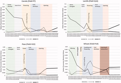
Figure 4 plots the DoP for representative canola, lentil, pea and wheat fields. Note that even very early in the growing season when canopies are sparse and leaves are only beginning to form, the DoP is less than 100%. Peas in particular have a lower DoP at the beginning of the season. Depolarization by the pea canopy is noted by mid-June, as 5 to 9 nodes have formed during stem elongation creating a dense canopy with interwoven stems, leaves and vines. The smaller lentil canopy and the early leaf development for canola do not create the same complex structure and thus early in the season the majority of scattering is still polarized for these two crops. For wheat, greater variability in DoP among fields is noted not only during early season but throughout the season. This variability may be due to differences in cultivars and variations in seeding dates for these different wheat varieties. For fields of canola, the DoP drops rapidly through stem elongation and flowering. During the development of pods, seed infilling and ripening, the proportion of scattered waves that are polarized is only 10–20%. This is expected considering not only the density of the canopy but the random orientation of canola pods as they intertwine and make walking through fields of canola in pod development nearly impossible. Canola is harvested by mid-August and the portion of polarized scattering increases. The DoP is still below 70% and some depolarization is most likely due to a large mat of residue left after harvest.

Figure 4. Plots of Degree of Polarization (DoP) for each date of RCM (CP Beam B) acquisition, acquired for the entire growing season. DoP is calculated using the Stokes parameters. Key phenological stages of growth are indicated for each crop type.

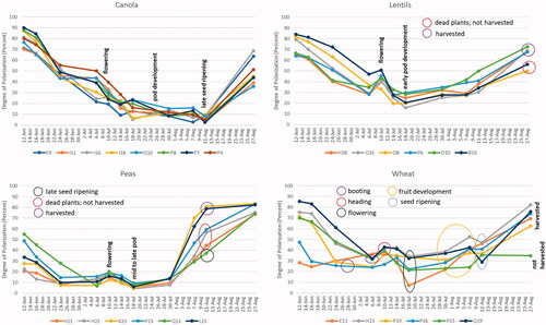
The DoP for lentils declines as the crop develops but for the majority of fields, the minimum DoP is above that reported for peas. As stated, lentils are overall a smaller canopy and although these smaller plants have a random structure, the size of leaves and stems are much smaller than the other three crop types. Of note, both peas and lentils exhibit a bump in DoP at the point of flowering. It is not clear why this occurs considering that the flowers that appear on lentil and pea canopies are sparse and small relative to the overall canopy biomass. Increases in the DoP are observed once lentils and peas are harvested. Even when plants are completely senesced (indicated as “dead plants” in Figure 4), DoP increases due to a decrease in contributions from these canopies as a result of low vegetation water content.

The DoP for wheat varies from field to field. Once the heads of the wheat emerge after booting, a slight increase in DoP is observed. Unlike peas and lentils, flowering in wheat reduces the DoP. As the grains of wheat infill DoP slowly increases, reaching 25–50% prior to seed ripening. In Figure 4, one wheat field is yet to be harvested and stands out among the other five fields which have been harvested. As with the other crops, post-harvest crop residue creates some depolarization.

Interpretation of stokes parameter responses

Often, classifications of crops with SAR images use intensity of backscatter at one or more linear polarizations. This is certainly the case for the Canadian operations which have used VV and VH backscatter (Davidson et al. 2017). However, results from the Kenaston site with RCM CP data demonstrated that the separation of crop types was improved when an RF classifier used all four Stokes parameters as compared to a classification run using only total intensity (S₀) or RH and RV backscatter (Table 5). As well, based on the top ten contributing parameters from the RF “All Stokes” classification, S₁, S₂ and S₃ were very important for the classification for all crop types. This result is interesting considering that the DoP (relative amount of polarized scattering to total scattering (polarized + unpolarized)) decreases as crops develop. Clearly the contributions of the polarized component of the EM scattering remain important to separate crops. Examining the physics behind why these Stokes parameters are helpful in identifying crops is informative, particularly when interpreted using measures of crop biophysical development such as BBCH stage. Phenology is an excellent indicator of the structure of the crop canopy.

Figure 5 displays three perspectives of the Poincaré 3 D plot for a representative canola field. Understanding the scattering within canola requires more perspectives as the handedness of rotation of the scattered wave changes mid-season. The plots for the other three crops are given in Figure 6. Recall that these 3 D plots are indications of the ellipticity, handedness (direction of rotation) and orientation of only the polarized part of the scattered wave, which decreases through to mid-season. Nevertheless, these characteristics of the polarized scattering, represented by Stokes parameters S₁, S₂ and S₃, perform well at separating crops likely due to their sensitivity to changing structure during crop development. In fact overall, S₁ and S₂ were predominant as being the most important of the Stokes parameters for classifying crops (Table 6).

Figure 5. Mapping of development stages of canola (field P7) on projections of the Poincaré 3 D spheres. Projections include (a) Left Handed Circular (LHC); (b) 135o; and (c) Right Handed Circular (RHC). For the 135o projection, circular scattering is located at the poles, linear scattering at the equator and elliptical scattering in all other locations on the plot.

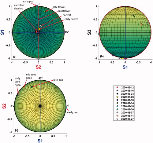
Figure 6. Mapping of crop development stages. Projections of the Poincaré sphere include Left Handed Circular (all crops) (left); 135o (lentils) or 00 (peas and wheat) (right).

Regardless of crop type, at the beginning (early leaf development) and end (harvest or plants fully senesced), scattered waves are circularly polarized. Raney et al. (2021) state that for a radar that transmits circular polarization, it is expected the largest of the three Stokes parameters to be S₃. We observe this for these agricultural fields during periods without a significant canopy present. Handedness of the scattered circular wave is LHC indicative of single scattering of the RHC transmitted wave early and late in the season. Figure 7 graphs the absolute values of these three Stokes parameters, and indeed early and late in the season, the magnitude of S₃ values are higher relative to S₁ and S₂ as predicted by Raney et al. (2021). A scattered wave is circularly polarized when H and V components are out of phase by 90° and amplitudes are equal. These nearly bare fields provide little structure that would create differences (in phase or intensity) of scattering between the horizontal and vertical components.

Figure 7. Plots of absolute values of Stokes parameters S₁, S₂ and S₃. The point at which S₃ declines to values close to S₁ is indicated as is the phenology stage for this point.

This circularly polarized scattering contributes to some classifications, likely at times when differences in emergence and harvesting are good indicators of crop type. In Table 6, the contributions of S₃ for classification of specific crops types are shown with late season (August 27 and 31) for pasture/forage, wheat, lentils and early season (June 1 and 9) for wheat, flaxseed, lentils indicated as important. Not surprisingly, S₃ for images acquired on June 1 (ranked 4th), August 27 (ranked 9th) and August 2 (ranked 10th) all appear in the top ten (Table 6).

The most significant change in scattering characteristics from canola is observed when the plants begin to flower. When flowering begins, scattered waves become slightly elliptical and as flowering progresses, ellipticity increases (waves become less and less circularly polarized). The waves still have a left handed rotation and the orientation of this elliptically polarized wave is horizontal, although late in flowering this orientation tilts slightly to an angle just off of horizontal. According to Raney et al. (2021), when the other Stokes parameters have considerably different values with respect to S₃, this indicates that backscatter includes target features with reflections at particular orientations. This is confirmed by Figure 7, when at mid-flowering S₃ declines and values of S₁ are equal to or greater than S₃. Recall that S₁ is the difference between the powers of the two received channels (H and V). When the amplitude of these two channels varies, and/or H and V reflections are out of phase (a phase difference between 0° and 90°), the reflection is elliptically polarized (Raney et al. 2021). Dasari and Lokam (2018) noted that in hybrid polarimetry, for every scattering event, the electric field loses circularity. We can expect that in a complex crop canopy many scattering events occurs. These observations are confirmed by the results listed in Table 6. For RCM images acquired early in July, S₁ is dominant in the top five important variables for canola (July 14 (1st ranking), July 6 (4th), and July 1st (5th)).

As pods develop, the leaves and flowers of the canola crop drop off the stems. Early in this growth stage, pods are small, but growing in size and infilling with seeds as pod development advances. Early in pod development, the scattered wave is linearly polarized (little ellipticity) and oriented horizontally. Yet in late pod development and during seed ripening, the backscattered wave has some ellipticity. Of particular interest, the complex canopy changes the handedness of rotation of the polarized component of the scattering (Figure 5b) to right handed, and the orientation of this ellipse is now at an angle between 45° and 90°. The change from circular to elliptical to linear and the change in handedness is easily observed in Figure 5c using a 3 D plot with a projection centered on the 135° polarization.

For wheat, LHC scattering is observed even as leaves and tillers develop. As the stems of the wheat plant elongate, scattered waves become slightly elliptical. During booting, the wheat head is developing within the flag leaf sheath but has not yet emerged and ellipticity increases only slightly. Ellipticity further increases from mid to late heading as wheat heads emerge. At flowering, as anthers appear, the scattered wave is primarily linearly polarized. The orientation of the scattered waves during heading and as the seeds of the wheat infill and ripen is between horizontal and 135°. At first glance, this orientation runs contrary to what might be expected given the predominantly vertical orientation of wheat stems. During ripening, grains in the head of the wheat become doughy and eventually hard. As the wheat heads gain weight (fruit development to ripening), heads tilt under this weight. The orientation of the scattered elliptically polarized wave varies among fields with some dominated by scattering between 90° and 135° and others between 0° and 135°. This variation is unsurprising given that the direction that the heads tilt, will vary from plant to plant. As stated, Figure 6 is capturing the polarized component of scattering which at heading represents about 45% of the total scattering (Figure 7). It appears that the heads are contributing significantly to the polarized scattering and likely the leaves of the wheat canopy which fall at different angles and orientations may be a more important contributor to unpolarized scattering. In Figure 7, the DoP increases when wheat heads develop and seeds infill confirming that not only total intensity but also the second, third and fourth Stokes parameters are important in identifying wheat fields (Table 6). S₁ declines and S₃ increases in late July and early August as wheat senesces and is harvested. These Stokes parameters, on these acquisition dates, are important in the overall classification (S₁ July 26th (1st rank); S₃ July 30 (5th); S₃ Aug 2nd (4th)).

The scattered energy from lentil canopies is mostly characterized by a change from circular polarizations (during stem elongation) to elliptical polarizations as this crop develops buds, then flowers, then pods. In Figure 6, the differences in the orientation of these elliptically scattered waves (horizontal, between 0° and 135° and between 90° and 135°) are indicative of a random orientation of buds and pods. Of note, however, is that as the seeds ripen, the scattered waves become less elliptical (more circular) and here orientation is consistently between 90° and 135°. As was noted for lentils, S₃ was identified five times in the top ten importance ranking. This underscores the contribution of circularly polarized waves in identifying this particular crop (August 2nd (1st importance, early ripening), August 27th (2nd), June 1 (3rd) (stem elongation), August 31st(5th) and July 30th (9th) (late pod)).

The amount of polarized scattering from fields of peas drops significantly by early July (Figure 6). Generally among all fields, ellipticity increases from stem elongation to flowering and pod development. However, the orientation of these elliptically polarized scattered waves varies significantly among the six sample fields and the location of these responses can be found in all quadrants of the 3 D Poincaré plots (not shown). This observation is likely due to the lower contributions of polarized energy during scattering when compared to the total scattering response (Figure 7). Not surprisingly, during the classification for peas the total intensity S₀ (polarized and unpolarized) delivered a more accurate classification for peas (user’s 99% and producer’s 87%) when compared to classification runs which used only S₁, S₂ and S₃ (user’s 85% and producer’s 81%). Additionally, S₀ is most prevalent in the importance for the peas class with July 6 (1st position, early flower), July 18 (3rd, mid pod), August 2 (4th), and June 1 (6th).

Overall as crops develop, changes in the characteristics of the polarized component of the EM scattered wave is observed. Early in the season responses are dominated by scattering which is mostly polarized and more specifically, circularly polarized. Insufficient canopy structure is present to create divergence of H and V scattering contributions. However, as plants buds then form flowers and seeds, the polarized component of total scattering decreases, and the polarized component of the wave becomes more elliptical. The RHC wave enters these canopies, where leaves, stems, flowers and fruit have created an ensemble of complex scattering elements. In particular, the orientation of these elements becomes varied. Differences in the amplitude and/or phase of the H and V components, due to this varied orientation, cause the scattered wave to rotate elliptically. Despite the fact that the amount of polarized energy is much lower than that of unpolarized energy once canopies gain biomass, S₁, S₂ and S₃ parameters are important contributors to crop classification. This observation is interesting and leads to the conclusion that the structural changes that occur during flowering and seed development are impacting how waves scatter. These results support research published more than a decade ago, which emphasized the importance of collecting SAR data during reproduction and seed development, to maximize classification accuracies (McNairn, et al. 2009).

Conclusions

In 2019, Canada launched the RADARSAT Constellation Mission (RCM) to support the operational mapping and monitoring of Canada’s marine approaches and landmass. Each of the three RCM satellites can image in a Compact Polarimetric (CP) mode, transmitting a right-handed circular (RHC) wave and receiving (coherently) scattering in H and V polarizations. The primary driver of including CP on this constellation was to support a desire from users to be able to image over wide swaths, but in a mode that provided greater polarization diversity. Although satellites like RCM, RISAT and SAOCOM include a CP imaging mode, testing the performance of these modes for mapping agricultural landscapes is limited. This study fulfills a need to better understand the capability of CP for crop mapping.

Seventeen RCM images were acquired in CP ScanSAR mode over a test site in western Canada. These images have a swath width of 125 km and nominal spatial resolution of 30 m. Parameters derived from these CP Single Look Complex (SLC) data included the four Stokes parameters (S₀, S₁, S₂ and S₃), three components of the m-chi decomposition (surface, double bounce and volume scattering) and backscatter intensities (RH; RV). A Random Forest (RF) classifier was applied to determine the accuracy of separating seven crop types (pasture/forage, barley, wheat, canola, flaxseed, peas and lentils). Different combinations of CP inputs were tested, leading to eight classification runs. Accuracies were compared among these RF runs, and were compared to a classification which used only satellite optical images.

An overall mapping accuracy of 95% was achieved for classification runs which used all Stokes or all m-chi parameters. These accuracies were about 2% lower than a classification using optical imagery with post-processing filtering. Both Stokes and m-chi parameter inputs to the RF classifier outperformed classification runs based upon inputs of backscatter intensity (either S₀ (total intensity) or RH + RV backscatter). Rankings of variable importance from the RF classifier indicated the contributions of each input to the success of both overall and crop specific classifications. Stokes parameters S₁ and S₂ ranked high in importance for all crops but were particularly important for canola, wheat and barley. For a smaller structured canopy like lentils, as well as for wheat, S₃ also ranked high in importance for identifying these two crops. The exception was peas where total scattering (S₀) was needed to achieve high accuracies.

To understand these classification outcomes, for wheat, canola, lentils and peas, the DoP was calculated from the Stokes parameters and the polarized scattering responses were plotted on the Poincaré sphere. These responses were interpreted relative to weekly phenology observations. Parsing the polarized and unpolarized contributions revealed that as the canopies developed significant structure, more of the scattering was returned unpolarized. Nevertheless, even during mid-season when the amount of polarized scattering was lower, the ellipticity and orientation characteristics of the polarized scattered waves varied among crops and changed as crop structure changed and phenology progressed. RCM transmits RHC waves, but canopy structure changed the phase and/or amplitude between H and V polarized scattering, leading to scattered waves which rotated with varying degrees of ellipticity. These observations support the rankings of importance for S₁ and S₂ in classifying crops.

This study demonstrated that RCM CP imagery can deliver crop classifications with high accuracy, confirming earlier results that were based on simulated CP data. The interpretation of the importance of the Stokes parameters to these classification lends support to the potential of CP to monitor crop development. Although this study is limited to one test site, these results should encourage broader efforts to adopt CP for operational mapping.

Disclosure statement

No conflict of interest was reported by the author(s).

References

- Agriculture and Agri-Food Canada. 2020. “Annual Space-Based Crop Inventory for Canada, 2009–2020.” Agroclimate, Geomatics and Earth Observation Division, Science and Technology Branch. https://open.canada.ca/data/en/dataset/ba2645d5-4458-414d-b196-6303ac06c1c9.
- Ballester-Berman, J.D., and Lopez-Sanchez, J.M. 2012. “Time series of hybrid-polarity parameters over agricultural crops.” IEEE Geoscience and Remote Sensing Letters, Vol. 9(No. 1): pp. 139–143. doi:10.1109/LGRS.2011.2162312.
- Boryan, C., Yang, A., Mueller, R., and Craig, M. 2011. “Monitoring US agriculture: The US department of agriculture, national agricultural statistics service, cropland data layer program.” Geocarto International, Vol. 26(No. 5): pp. 341–358. doi:10.1080/10106049.2011.562309.
- Bouchemakh, L., Smara, Y., Boutarfa, S., and Hamadache, Z. 2008. “A comparative study of speckle filtering in polarimetric radar SAR images.” IEEE Proceedings of the 3rd International Conference on Information and Communication Technologies: From Theory to Applications ICTTA’08, Damascus, Syria, 1–6 May 2008. doi:10.1109/ICTTA.2008.4530040.
- Breiman, L. 2001. “Random Forests.” Machine Learning, Vol. 45(No. 1): pp. 5–32. doi:10.1023/A:1010933404324.
- Brisco, B., Li, K., Tedford, B., Charbonneau, F., Yun, S., and Murnaghan, K. 2013. “Compact polarimetry assessment for rice and wetland mapping.” International Journal of Remote Sensing, Vol. 34(No. 6): pp. 1949–1964. doi:10.1080/01431161.2012.730156.
- Charbonneau, F.J., Brisco, B., Raney, R.K., McNairn, H., Liu, C., Vachon, P.W., Shang, J., et al. 2010. “Compact polarimetry overview and applications assessment.” Canadian Journal of Remote Sensing, Vol. 36(No. sup2): pp. S298–S315. doi:10.5589/m10-062.
- Chirakkal, S., Haldar, D., and Misra, A. 2017. “Evaluation of hybrid polarimetric decomposition techniques for winter crop discrimination.” Progress in Electromagnetics Research M, Vol. 55: pp. 73–84. doi:10.2528/PIERM17011603.
- Cloude, S.R., Goodenough, D.G., and Chen, H. 2012. “Compact decomposition theory.” IEEE Geoscience and Remote Sensing Letters, Vol. 9(No. 1): pp. 28–32. doi:10.1109/LGRS.2011.2158983.
- Cloude, S.R., and Pottier, E. 1996. “A review of target decomposition theorems in radar polarimetry.” IEEE Transactions on Geoscience and Remote Sensing, Vol. 34(No. 2): pp. 498–518. doi:10.1109/36.485127.
- Collett, E. 2005. Field Guide to Polarization. Bellingham, WA: SPIE Press.
- Dasari, K., and Lokam, A. 2018. “Exploring the capability of compact polarimetry (hybrid pol) C band RISAT-1 data for land cover classification.” IEEE Access., Vol. 6: pp. 57981–57993. doi:10.1109/ACCESS.2018.2873348.
- Dave, V.A., Haldar, D., Dave, R., Misra, A., and Pandey, V. 2017. “Cotton crop biophysical parameter study using hybrid/compact polarimetric RISAT-1 SAR data.” Progress in Electromagnetics Research M, Vol. 57: pp. 185–196. doi:http://doi.org/10.2528/PIERM16121903.
- Davidson, A. M., Fisette, T., McNairn, H., and Daneshfar, B. 2017. Detailed crop mapping using remote sensing data (Crop Data Layers). In Handbook on remote sensing for agricultural statistics (Chapter 4), edited by J. Delincé. Rome: Handbook of the Global Strategy to Improve Agricultural and Rural Statistics (GSARS).
- De, S., Kumar, V., and Rao, Y. 2014. “Crop classification using RISAT-1 hybrid polarimetric SAR Data.” Eursar 2014, p. 5.
- Deschamps, B., McNairn, H., Shang, J., and Jiao, X. 2012. “Towards operational radar-only crop type classification: Comparison of a traditional decision tree with a random forest classifier.” Canadian Journal of Remote Sensing, Vol. 38(No. 1): pp. 60–68. doi:10.5589/m12-012.
- Dingle Robertson, L., Davidson, A. M., McNairn, H., Hosseini, M., and Mitchell, S. 2019. "Compact polarimetry for agricultural mapping and inventory: Preparation for RADARSAT constellation mission." IGARSS 2019 - 2019 IEEE International Geoscience and Remote Sensing Symposium, 5851–5854, 28 July–2 August 2019. doi:10.1109/IGARSS.2019.8898631.
- Dingle Robertson, L., Davidson, A.M., McNairn, H., Hosseini, M., Mitchell, S., De Abelleyra, D., Verón, S., and Cosh, M.H. 2020a. “Synthetic Aperture Radar (SAR) image processing for operational space-based agriculture mapping.” International Journal of Remote Sensing, Vol. 41(No. 18): pp. 7112–7144. doi:10.1080/01431161.2020.1754494.
- Dingle Robertson, L., Davidson, A.M., McNairn, H., Hosseini, M., Mitchell, S., De Abelleyra, D., Verón, S., et al. 2020b. “C-band synthetic aperture radar (SAR) imagery for the classification of diverse cropping systems.” International Journal of Remote Sensing, Vol. 41(No. 24): pp. 9628–9649. doi:10.1080/01431161.2020.1805136.
- Doyon, M., Smyth, J., Kroupnik, G., Carrie, C., Sauvageau, M., Levesque, J.-F., Babiker, F., et al. 2018. “RADARSAT CONSTELLATION MISSION: Toward launch and operations.” 15th International Conference on Space Operations, May 2018. doi:10.2514/6.2018-2605.
- Fisette, T., McNairn, H., and Davidson, A. M. 2015. An operational annual space-based crop inventory based on the integration of optical and microwave remote sensing data: Protocol document. Ottawa: Agriculture and Agri-Food Canada Publication.
- Freeman, S., and Durden, L.A. 1998. “Three-component scattering model for polarimetric SAR Data.” IEEE Transactions on Geoscience and Remote Sensing, Vol. 36(No. 3): pp. 963–973. doi:10.1109/36.673687.
- Gagnon, L., and Jouan, A. 1997. “Speckle filtering of SAR images - A comparative study between complex-wavelet-based and standard filters.” SPIE Proceedings. #3169, “Wavelet Applications in Signal and Image Processing V,” San Diego. doi:10.1117/12.279681.
- Hu, Y., Tao, V., and Croitoru, A. 2004. “Understanding the rational function model: methods and applications.” Environmental Science. ISPRS.org, Corpus ID: 2702825. ISC.ca, https://www.isc.ca/signedinhome/help/land/pages/landdescriptions.aspx (downloaded December 2021).
- Magagi, R., Berg, A.A., Goïta, K., Bélair, S., Jackson, T.J., Toth, B.M., Walker, A.S., et al. 2013. “Canadian experiment for soil moisture in 2010 (CanEx-SM10): Overview and preliminary results.” IEEE Transactions on Geoscience and Remote Sensing, Vol. 51(No. 1): pp. 347–363. doi:10.1109/TGRS.2012.2198920.
- Mahdianpari, M., Mohammadimanesh, F., McNairn, H., Davidson, A.M., Rezaee, B., Salehi, S., and Homayouni, S. 2019. “Mid-season crop classification using dual-, compact-, and full-polarization in preparation for the RADARSAT constellation mission (RCM).” Remote Sensing, Vol. 11(No. 13): pp. 1582–1608. doi:10.3390/rs11131582.
- McNairn, H., Shang, J., Jiao, X., and Champagne, C. 2009. “The Contribution of ALOS PALSAR Multi-polarization and Polarimetric Data to Crop Classification.” IEEE Transactions on Geoscience and Remote Sensing, Vol. 47(No. 12): pp. 3981–3992. doi:10.1109/TGRS.2009.2026052.
- McNairn, H., and Shang, J. 2016. “Multitemporal remote sensing: Methods and applications.” In A review of multitemporal synthetic aperture radar (SAR) for crop monitoring, edited by Y. Ban, vol. 20, 317–340. Cham: Springer. doi:10.1007/978-3-319-47037-5_15.
- Meier, U. 2001. Growth stages of mono-and dicotyledonous plants: BBCH monograph. Oxford, UK: Federal Biological Research Centre for Agriculture and Forestry.
- Millard, K., and Richardson, M. 2015. “On the importance of training data sample selection in random forest image classification: A case study in peatland ecosystem mapping.” Remote Sensing, Vol. 7(No. 7): pp. 8489–8515. doi:10.3390/rs70708489.
- Natural Resources Canada, Canada Centre for Mapping and Earth Observation. 2020. “Earth observation data management system SAR toolbox.” https://www.nrcan.gc.ca/earthobservation (accessed 2020).
- Quinlan, J.R. 1990. “Decision trees and decision making.” IEEE Transactions on Systems, Man, and Cybernetics, Vol. 20(No. 2): pp. 339–346. doi:10.1109/21.52545.
- Raney, R.K. 2006. “Dual-polarized SAR and Stokes parameters.” IEEE Geoscience and Remote Sensing Letters, Vol. 3(No. 3): pp. 317–319. doi:10.1109/LGRS.2006.871746.
- Raney, R.K. 2007. “Hybrid-polarity SAR architecture.” IEEE Transactions on Geoscience and Remote Sensing, Vol. 45(No. 11): pp. 3397–3404. doi:10.1109/TGRS.2007.895883.
- Raney, R.K. 2019. “Hybrid dual-polarization synthetic aperture radar.” Remote Sensing, Vol. 11(No. 13): pp. 1521. doi:10.3390/rs11131521.
- Raney, R. K., Cahill, J. T. S., Patterson, G. W., and Bussey, D. B. J. 2012. “The m-chi decomposition of hybrid dual-polarimetric radar data.” IEEE International Geoscience and Remote Sensing Symposium, Munich, Germany, 22–27. doi:10.1029/2011JE003986.
- Raney, R.K., Brisco, B., Dabboor, M., and Mahdianpari, M. 2021. “RADARSAT constellation mission’s operational polarimetric modes: A user-driven radar architecture.” Canadian Journal of Remote Sensing, Vol. 47(No. 1): pp. 1–16. doi:10.1080/07038992.2021.1907566.
- Saskatchewan Ministry of Agriculture, Annual Report for 2020–2021. n.d. https://publications.saskatchewan.ca/api/v1/products/113765/formats/128171/download (downloaded February 2022).
- Shang, J., McNairn, H., Champagne, C., and Jiao, X. 2009. “Advances in geoscience and remote sensing.” In Application of multi-frequency synthetic aperture radar (SAR) in crop classification, edited by G. Jedlovec, 557–568. Rijeka, Croatia: InTech.
- Shook, K., Pomeroy, J.W., Spence, C., and Boychuk, L. 2013. “Storage dynamics simulations in prairie wetland hydrology models: evaluation and parameterization.” Hydrological Processes, Vol. 27(No. 13): pp. 1875–1889. doi:10.1002/hyp.9867.
- Sun, S., Liu, R., Yang, C., Zhou, H., Zhao, J., and Ma, J. 2016. “Comparative study on the speckle filters for the very high-resolution polarimetric synthetic aperture radar imagery.” Journal of Applied Remote Sensing, Vol. 10(No. 4): pp. 045014. doi:10.1117/1.JRS.10.045014.
- Tetlock, E., Toth, B., Berg, A., Rowlandson, T., and Ambadan, J.T. 2019. “An 11-year (2007–2017) soil moisture and precipitation dataset from the Kenaston Network in the Brightwater Creek basin, Saskatchewan, Canada.” Earth System Science Data, Vol. 11(No. 2): pp. 787–796. doi:10.5194/essd-11-787-2019.
- Touzi, R., Lapointe, M., Nedelcu, S., Fobert, M. A., and Cote, S. 2021. “Assessment and calibration of RCM compact.” 42 Canadian Symposium on Remote Sensing, Virtual Presentation, Yellowknife, NWT, June 22–24, 2021.
- Uppala, D., Venkata, R.K., Poloju, S., Sai, S., Rama, M.V., and Dadhwal, V.K. 2016. “Discrimination of maize crop with hybrid polarimetric RISAT1 data.” International Journal of Remote Sensing, Vol. 37(No. 11): pp. 2641–2652. doi:10.1080/01431161.2016.1184353.
- Waldner, F., De Abelleyra, D., Verón, S.R., Zhang, M., Wu, B., Bartalev, P.D., Lavreniuk, S., et al. 2016. “Towards a set of agrosystem-specific cropland mapping methods to address the global cropland diversity.” International Journal of Remote Sensing, Vol. 37(No. 14): pp. 3196–3231. doi:10.1080/01431161.2016.1194545.
- Wang, H., Zhou, Z., Turnbull, J., Song, Q., and Qi, F. 2015. “Three-component decomposition based on stokes vector for compact polarimetric SAR.” Sensors, Vol. 15(No. 9): pp. 24087–24108. doi:10.1109/EuRAD.2015.7346240.
- Xie, L., Zhang, H., Li, H., and Wang, C. 2015. “A unified framework for crop classification in southern China using fully polarimetric, dual polarimetric, and compact polarimetric SAR data.” International Journal of Remote Sensing, Vol. 36(No. 14): pp. 3798–3818. doi:10.1080/01431161.2015.1070319.