Observations of Thin First Year Sea Ice Using a Suite of Surface Radar, LiDAR, and Drone Sensors

Abstract

Arctic sea ice is rapidly transitioning into a perennial first year ice pack and this is being observed with satellite remote sensing. Satellite image interpretation requires accurate knowledge of the physical conditions and how they give rise to the microwave scattering response that is present within a single image pixel. This study addresses this issue through a focused remote sensing study of thin first year sea ice. We present results from an experiment that fused datasets from surface-based C- and Ku-band polarimetric scatterometers, LiDAR, and drone-based optical and thermal infrared sensors. We grew frost-flower-covered thin first year sea ice in a mesocosm facility and measured the time-series evolution of C- and Ku-band scattering response as it evolved into snow-covered sea ice. Drone surveys, LiDAR scans, and physical sampling provided complementary characterization of the ice. Results quantify the sensitivity of C- and Ku-band to the presence of frost flowers, the addition of snow, and the meteorological conditions. Drone surveys enhanced the characterization by rapidly performing observations over a larger representative region. In essence, they are helping to close the gap between surface-based sensing and satellite imagery. Furthermore, this study complements and enhances our understanding of the snow-covered sea ice system.

RESUME

La banquise arctique est en train de se transformer rapidement en une banquise pérenne de première année, ce constat est observé grâce à la télédétection par satellite. L’interprétation d’images satellitaires nécessite une connaissance précise des conditions physiques de la glace et de leur signature de diffusion dans un seul pixel d’image micro-ondes. Cette étude aborde cette question au moyen d’une étude ciblée de la glace de mer mince de première année. Nous présentons les résultats d’une expérience qui a fusionné des ensembles de données provenant de diffusiomètres polarimétriques de surface en bande C et Ku, de LiDAR et de capteurs infrarouges optiques et thermiques installés sur des drones. Nous avons aussi généré de la glace de mer mince couverte de fleurs de gel dans une installation de mésocosme et mesuré l’évolution des séries chronologiques de la réponse de diffusion en bandes C et Ku à mesure que la glace évoluait en glace de mer enneigée. Les relevés par drone, les balayages LiDAR et l’échantillonnage physique ont fourni une caractérisation complémentaire de la glace. Les résultats permettent de quantifier la sensibilité des bandes C et Ku à la présence de fleurs givrées, à l’ajout de neige et aux conditions météorologiques. Les relevés par drone ont amélioré la caractérisation en effectuant rapidement des observations sur une vaste région représentative. Essentiellement, ils aident à combler l’écart entre les mesures de surface et l’imagerie satellitaire. De plus, cette étude complète et améliore notre compréhension du système glace de mer-couvert nival.

Introduction

Arctic sea ice is declining in extent and thickness, which has transitioned the ice cover from one predominantly comprised of older, thicker multiyear sea ice to one increasingly comprised of younger, thinner seasonal ice types (Kwok 2018). The transition to thinner ice types modifies the surface energy balance and makes the ice cover less resilient to melt (Alexeev et al. 2017). Furthermore, this change affects the sea ice ecosystem (Steiner et al. 2021) and changes the risk that sea ice presents to vessels operating in Arctic waters (Stevenson et al. 2019; AMAP 2007).

Thin first year sea ice (FYI), which is also known as White Ice, may be from 30 to 70 cm thick (WMO 2014). The surface of thin FYI can be bare, snow-covered, or covered by frost flowers (FF). FF, which are highly saline crystal structures, may form on the thin sea ice when cold temperatures, low wind speeds, and high humidity are present (Domine et al. 2005; Galley et al. 2015). They are known to modify the thermodynamic balance and act as conduits to expose sea water salts to the atmosphere (Douglas et al. 2012). Studies into the physical, thermodynamic, and microwave scattering behavior of FF have shown that these features are highly detectable using radar (Isleifson et al. 2018; Isleifson et al. 2014). They are a transient phenomenon, typically lasting a few days at most. Natural snowfall and wind action result in the integration of these features into the basal layer of snow on sea ice. In this situation, the basal layer has a high brine content which affects the thermophysical make-up of the sea ice surface, and consequently, microwave interactions.

In addition to sea ice decline, snow cover throughout the Arctic is anticipated to become both thinner and more saline, due to the effects of climate change and the reduction of multiyear sea ice (Blanchard-Wrigglesworth et al. 2015). Snow on sea ice is a critical aspect of the ocean-sea ice-atmosphere system (Barber et al. 1998). It acts as a thermal insulator, slowing sea ice growth throughout winter, and has a high albedo, affecting the surface energy balance and sea ice melt in the spring season (Stroeve et al. 2014).

Microwave remote sensing has been established as an effective tool for observing sea ice under different physical conditions (Barber 2005). One of the goals of Arctic remote sensing is to derive the physical and thermodynamic state of sea ice, such that the conditions can be used to understand how the ice is changing over time and space. This information can be used in the creation of ice charts and maps for transportation and operational sea ice monitoring (Shokr et al. 2022; Scheuchl et al. 2004).

Depending on the sea ice physical and thermodynamic state, microwaves will exhibit specific scattering behaviors, which are commonly known as the scattering signature or backscatter response. The backscattering response from bare sea ice is dependent on the physical and thermodynamic state of the ice; however, when sea ice is covered with surface features, such as FF and snow, the backscattering response changes dramatically because it is dependent on the combination of the surface layer and underlying ice physical properties (e.g., Drinkwater et al. 1992; Isleifson et al. 2010; Nghiem et al. 1997; Nghiem et al. 1995; Nghiem et al. 1997; Onstott 1992). Sea ice deformation mechanisms, including ridges and leads, are known to have significantly different backscattering responses when compared to level undeformed sea ice floes. Ridging can increase the backscatter level, while the opening of a lead can present a relative drop in backscatter, followed by a subsequent increase as the sea ice forms (Melling 1998).

Surface features can cause distinct backscattering responses at different frequencies, incidence angles, and polarizations. During sub-zero temperatures, at higher frequencies such as Ku-band, FYI scattering may be dominated by volume scattering that occurs within snow layers or by surface scattering that occurs at the roughened air-FF interface. When FYI is free of surface covering, the bare layer is often highly saline, leading to surface scattering at the air-ice interface as the dominate scattering mechanism, though the backscattering response is lower than that of FF due to the smoother surface. At lower frequencies, such as C-band, the microwave radiation penetrates deeper into the surface layer (snow or FF) than at higher frequencies, resulting in a multilayer type of interface scattering (Komarov et al. 2015). These interactions are complex, and in an effort to establish unique scattering signatures, many field studies and campaigns have had the goal to measure the microwave scattering response of snow-covered sea ice under a variety of conditions.

Backscatter from snow cover on sea ice has a frequency dependence, due to the size and geometry of snow grains and other snow properties. While the backscatter measured from dry snow is similar for X- and C-band frequencies (Lytle et al. 1993; Beaven et al. 1993; Grenfell et al. 1998), Grenfell reported that grain size and layer structure of snow are the major factors that affect the radar backscatter. The Ku-band radar studies from CRREL laboratory experiments (Lytle et al. 1993; Beaven et al. 1993) demonstrated the effects of snow cover over the ice surface. They found that the dominant scattering in Ku-band originated from the snow/sea ice interface when there was a cold dry snow cover present on the ice.

Time-series observations are a key aspect of remote sensing, as factors can change as a result of diurnal variations, seasonal variations, and precipitation events. Despite significant progress in the study of sea ice scattering at various microwave frequencies over time and space (Barber et al. 1995; Bredow and Gogineni 1990; Nandan et al. 2016; Yackel et al. 2017; King et al. 2013; Yueh et al. 2009), research on the early stages of ice growth, specifically thin FYI that is usually covered with FF and snow, remains limited. This deficiency represents a major gap in our knowledge of the heat flux between the ocean, ice, and atmosphere during the freeze-up and early winter seasons. Understanding the temporal evolution of multifrequency scattering processes of sea ice is critical for accurately predicting and modeling the thermodynamic behavior of sea ice, as well as its impacts on the global climate (Barber 2005).

Beyond microwave remote sensing, optical remote sensing can also be used to observe the state of the sea ice surface. For more than a decade, light detection and ranging (LiDAR) has been a valuable tool for measuring and analyzing surface topographies and surface roughness under several fields of study (e.g., Calders et al. 2014; Hudak et al. 2009; Landy et al. 2015). With recent development in LiDAR-based technology, terrestrial sensors are being routinely tested under Arctic winter conditions (−20 °C to −30 °C temperatures; high winds; etc.) and becoming a reliable source for measuring and investigating sea ice topographic and roughness data (see Asihene et al. 2022; Landy et al. 2015; Trujillo et al. 2016). Results from these previous studies demonstrate the capability and complementarity of terrestrial LiDAR data for analyzing minute variability in sea ice surface characteristics, and how such analyses can provide insight toward an increased understanding of surface dynamics in sea ice.

Advances in drone-based technology have expanded the potential for sensors to survey moderately sized regions of snow-covered sea ice (i.e., hundreds of meters) (Jenssen et al. 2020; Harasyn et al. 2020). Common instruments include cameras with RGB channels and thermal infrared sensors. The benefit of using drone surveys is in their capability of rapidly performing observations over a larger representative region than can be obtained through surface-based sensors or discrete observation points. In effect, these platforms are helping to close the gap between surface-based sensing and satellite imagery.

This manuscript presents results from an experiment on thin first year sea ice with FF that was subsequently covered by snow. We used surface-based radar instruments operating in the microwave C-band and Ku-band, as they match those of existing and upcoming satellite missions (C-band: ASCAT, RADARSAT-2, RADARSAT Constellation Mission and Sentinel-1A/B; Ku-band: OSCAT, QuikSCAT, CryoSat-2), and have operating characteristics that are similar to these payloads. By using near-surface radar systems to measure the backscattering response, in conjunction with physical sampling and local meteorological observations, we can elucidate how the physical and thermodynamic state of the snow-covered sea ice give rise to the C-band and Ku-band scattering behaviors. Furthermore, to augment our data collection, we deployed terrestrial LiDAR and drone-based sensors to acquire complementary data. We attempt to use these sensors to explain the connections between discrete point measurements of physical properties and the distribution across the sea ice surface that are observed by our radar systems.

Ultimately, we addressed the following three objectives in this experiment:

1. Measure and evaluate the temporal evolution of C-band and Ku-band scattering responses of a thin FYI surface for a variety of surface features (e.g., FF and snow).

2. Examine the link between the temporally evolving sea ice, FF, and snow physical properties and the measured scattering response.

3. Assess how multi-sensor fusion, through the use of drone imagery, terrestrial LiDAR, and surface-based scatterometers, can complement and enhance our understanding of the snow-covered sea ice system.

Data and methods

Description of the facility and instrument configuration

The Sea-ice Environmental Research Facility (SERF) is a mesocosm system that is located at the University of Manitoba, in Winnipeg, Manitoba, Canada (see Figure 1). The main feature is an outdoor pool that can be filled with seawater, which freezes into sea ice during the cold temperatures of the Winnipeg winter months. The pool is 9.1 m by 18.2 m and has a depth of 2.45 m. During our experiments, the pool was filled with artificial seawater that was formulated through a combination of local groundwater and added salts. The artificial seawater has the ionic composition, pH, and alkalinity of natural Arctic Ocean surface water. The pool has a series of pumps that can be used to circulate the water and a heater to maintain open water conditions, even in the ambient Winnipeg winter temperatures. A large dome cover, which is fully retractable, can be used to control the rate of sea ice growth and the amount of precipitation that falls into the pool water (or ice). An automated meteorological station monitors the local ambient weather conditions. SERF has facilitated sea ice remote sensing experiments under a variety of conditions (e.g., Isleifson et al. 2018; Isleifson et al. 2014; Asihene et al. 2022). These studies have focused on remote sensing of frost flowers and detection of oil spills (in a separate, adjacent tub of water). Previous remote sensing experiments have used a C-band polarimetric scatterometer, in conjunction with a terrestrial LiDAR system to characterize the surface roughness. We have recently added opportunistic drone flights to acquire site images. In 2022, we performed a radar calibration experiment using an L-band, C-band, and Ku-band scatterometer (Isleifson et al. 2023). This manuscript presents one of the first multi-frequency radar experiments at the facility.

Figure 1. SERF site map showing; Ku-band scatterometer (yellow), C-band scatterometer (red), terrestrial LiDAR scanner (light blue), drone and sensors, and locations of GCPs for drone image rectification.

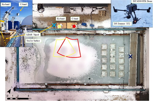
During this experiment, we used a suite of instruments, consisting of a C-band scatterometer, a Ku-band scatterometer, terrestrial LiDAR, a drone-based RGB and thermal sensor, and performed physical sampling measurements to characterize a thin FYI sea ice cover in the SERF pool. In previous studies, we have retracted the main pool cover to let the sea ice grow under ambient conditions. In this experiment, we allowed the ice to form underneath the cover, which promoted the formation of FF on the young ice. Once the ice was suitably thick (∼27 cm), we retracted the cover and began our scatterometer and drone measurements over the sea ice.

Scatterometer configuration

We used C-band and Ku-band polarimetric scatterometers to measure the microwave scattering response of the sea ice in the SERF pool. The instruments were developed by ProSensing, Inc. The C-band scatterometer has a center frequency of 5.5 GHz. It uses a dual-polarized reflector antenna with a half-power beamwidth (HPBW) of 5.7° in both the E- and H-planes, which correspond to the V-polarization and H-polarization, respectively. The Ku-band scatterometer has a similar configuration and has a slightly narrower beamwidth (4.3°). Additional details on the technical parameters are provided in Table 1.

Table 1. Polarimetric scatterometer system parameters.

Parameter	C-SCAT	Ku-SCAT
Center frequency	5.5 GHz	17.2 GHz
Sweep bandwidth	500 MHz	500 MHz
Transmitted power	−6 dBm	−10 dBm
Range resolution	30 cm	30 cm
Antenna type	Parabolic reflector with dual polarized feed
Antenna half-power beamwidth	5.7°	4.3°
Cross-polarization isolation	>28 dB	>29 dB
Polarization modes	VV, VH, HV, HH
External calibration	Trihedral corner reflector
Sensitivity at 5 m range	−56 dB m^2/m^2	−42 dB m^2/m^2

The systems were mounted on a platform on the north side of the pool (i.e., looking south) at a height of 2.4 m above the sea ice surface (see Figure 1). The C-band footprint size, calculated using the HPBW and assumed flat surface on the sea ice, ranges from ∼0.11 m² at 30° to 0.46 m² at 55°. Similarly, the Ku-band footprint size ranges from ∼0.06 m² at 30° to 0.26 m² at 55°. Measurements were conducted with 40° swaths in azimuth and elevation incidence angles were set at discrete increments of 5°, from 25° to 55° from nadir. In quality control review, we established that the lower incidence angles were affected by the pool railing, and therefore we only consider data from an incidence angle of 30° and up. We configured the systems to have overlapping footprints on the sea ice surface. In operation, the backscattered power was measured, and the covariance matrix was calculated to obtain the VV, HV, VH, and HH normalized radar cross sections (NRCS). Scans were collected every 15 minutes, starting from 09:00 on February 12 and continuing until the experiment end at 17:00 on February 23. In the data post-processing, we used a moving average filter (n = 4) to present the time-series trend of the radar data. We used a trihedral corner reflector for external calibration and an internal delay line calibration to account for any system drift. The manufacturer-tested sensitivity of the C-band instrument is −56 dB m²/m² and the Ku-band instrument is −42 dB m²/m² at 5 m range. This type of scatterometer system has been used in several field campaigns and its utility and processing have been discussed in Isleifson et al. (2010, 2018). Although fully polarimetric data, including Covariance and Mueller matrices, were collected, this manuscript focuses on the NRCS and their connections to the physical phenomenon observed in the SERF pool.

Drone measurements

A DJI Zenmuse XT2 was mounted on a DJI M300 RTK drone to collect simultaneous RGB optical and thermal infrared (TIR) imagery of the ice surface (Figure 1). The Zenmuse XT2 used a FLIR TAU 2 thermal sensor (640 × 512 pixels) to capture radiometric JPEGs (RJPEG), which have radiometric information stored within the metadata that is used to convert image pixels into temperature values (https://www.dji.com/ca/zenmuse-xt2/specs; accessed November 24, 2022). TIR measurements were captured in the 7.5–13.5 µm spectral range, with a < 50 mK sensitivity. In combination with the thermal sensor, the XT2 is equipped with a 12 MP RGB camera, which is triggered in synchronization with the thermal sensor.

The drone system was manually flown in a gridded pattern at an altitude of 5 m above the ice surface. The XT2 camera was manually triggered to achieve an image overlap of 70% in both the along track and across track directions. Images were processed in Pix4D Mapper (v 4.5.6), which used structure from motion (SfM) to generate RGB and TIR stitched ortho-mosaics. Ortho-mosaics were geo-rectified using ground control points (Leica reflective panels, Figure 1) distributed at the four corners of the study area, which were also used to rectify terrestrial LiDAR scans to drone orthomosaics. Geo-corrected mosaics were manipulated in ArcMap (v 10.8.1) for figure generation. Spot measurements of temperature from TIR mosaics were taken in ArcMap, which were used in combination with in situ temperature measurements for linear correction of TIR drone data (Li et al. 2022). In this experiment, the measurement accuracy was calculated to be 0.9 °C by analyzing TIR imagery, in conjunction with surface temperature readings, over a snow-covered surface.

The initial coverage of FF was determined by running a supervised classification on the first two RGB aerial mosaics collected over the pool. From this, we established the percent coverage of FF within the combined scatterometer field of view.

LiDAR measurements

A Leica ScanStation P40 LiDAR system was used for measurement of the ice surface roughness. The Leica P40 sensor operates at a wavelength of 658 nm (visible) and 1550 nm (invisible), recording the time-of-flight for each pulse and reflection. These pulses consistently reflect off surfaces such as snow and ice but are often absorbed by water (Perovich 1998). The scanner was mounted on a tripod along the north edge of the pool (directly adjacent to the scatterometer set up, shown in Figure 1) and positioned at a height of 1.9 m above the ice surface.

Surface roughness point cloud data were acquired during the scan operations. Two scales of point resolution were used for each series of scans including a larger area scan at 0.01 × 0.01 m covering the entire pool surface and general surrounding, and a smaller, higher interest area scan at 0.002 × 0.002 m point spacing covering the sections aligned with the scatterometer measurements. These resolutions were chosen based on a suitable range described and tested in previous ice roughness analyses from point cloud data (Landy et al. 2015; Isleifson et al. 2018). The vertical point acquisition of the LiDAR surface data was equal to the horizontal point acquisition at 0.002 m for all high-resolution scans. Scans were conducted with a pulse range of 10 m (0.4 mm reduction noise). All but one series of scans were conducted before sunrise under artificial lighting at the time of this experiment.

After registering each series of scans, outlying points located above or below the pool ice surface were removed through both manual noise reduction and Octree outlier filtering algorithms (CloudCompare 2022). Sections of the point cloud selected for further processing and analysis were within the area aligned with the scatterometer to coincide with the RADAR footprints as closely as possible. Using LAStools (Isenburg 2014), these subsections were resampled to 5 million points and gridded to 0.002 m 0.002 m cells using linear interpolation. Six representative regions were selected within the scatterometer footprint to give detailed information on two incidence angles (nominally, 35° and 45°). For these regions, the root mean square heights from a mean level through the grid were calculated, based on the algorithms of Landy et al. (2015), and an assessment of the surface features was provided to support the analysis of the scatterometer data.

Physical measurements

We monitored the local meteorological conditions and conducted physical sampling of the sea ice and its coverage to characterize it. Automated meteorological measurements included air temperature and relative humidity (Vaisala HMP45C, temperature accuracy = ±0.4 °C, relative humidity accuracy = ±2%). The surface temperature of the sea ice was measured using an Apogee SI-111 infrared sensor (calibration uncertainty = 0.02 °C, measurement repeatability < 0.05 °C).

The surface was covered with FF and later with snow. To detect snow and ice surface wetness, we touched a Kimwipe™ (a disposable, high-quality tissue paper) to the surface and observed if any liquid wicked up into the material (Isleifson et al. 2018). FF samples were taken from the sea ice surface using a pre-cleaned plastic spatula and placed into sterilized Whirl-Pak water-tight bags. Bulk snow samples were extracted using a 2-cm cutter. Ice surface samples were obtained by scraping the ice with an aluminum spatula and placed into sterilized Whirl-Pak water-tight bags. Physical samples were taken in triplicate (with one exception for the first FF samples). The conductivity and temperature of the meltwater from each sample were measured using a conductivity meter (Thermo Scientific Orion Star A212). The sample salinities were calculated from the conductivity according to the formulation of Fofonoff (1985).

Ice cores were extracted using a Kovacs Enterprise Mark II coring system (9 cm diameter). Temperatures were measured by extracting an ice core, drilling a small hole into the core at 5-cm intervals, and using a probe (Traceable Digital Thermometer, Control Company, accuracy of ±0.05 °C) to measure temperature. Ice salinities were obtained by segmenting the ice core into 5 cm sections using a thin Japanese-style rip/crosscut saw and storing them in containers. The ice was melted indoors in the SERF laboratory and the conductivity was measured. Salinities were calculated using the expressions from Fofonoff (1985). A bulk estimate of the core salinity was obtained by averaging the measurements of the entire core.

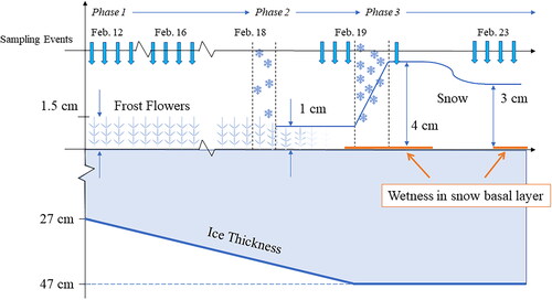
Physical sampling was performed four times per day on four separate days (blue arrows Figure 2). Physical samples were collected eight times during the first phase of the experiment when FF were present at the surface of the ice, three times during the second phase after the initial snow layer accumulated, and finally five more times during the third phase after the final snow layer was added. FF heights, snow thickness, and ice thickness are presented in Figure 2, while FF, snow, and sea ice salinities are shown in Figure 5.

Figure 2. Time-series evolution of the snow and sea ice thickness (sketch). Sampling times are denoted with blue arrows. Snowfall events are denoted by falling snowflakes.

Summary of data collection

Scatterometer and meteorological data were collected continuously through the experiment. Physical measurements, drone flights, and LiDAR measurements were discrete events that were scheduled to give a diurnal characterization on four separate days. We are limited in the amount of snow and ice sampling that can be performed on the SERF pool before we would begin to affect the preserved region for scatterometer measurements. A balance in the discrete time-series must be achieved to sufficiently sample and understand the physical changes and we acknowledge that there are bounds to our conclusions based on these limitations. A summary of the physical sampling, drone flights, and LiDAR scan times is provided in Table 2. Sufficient overlap was not achieved for TIR imagery on February 12 at 14:00, February 19 at 19:00, and February 23 at 06:00, therefore stitched thermal orthomosaics could not be generated for these flights.

Table 2. Discrete sampling event summary.

Date	Time	Physical measurements	RGB data	TIR data	LiDAR
February 12	06:00	X	x	x	x
	10:00	X
	14:00	X	x		x
	19:00	X
February 16	06:00	X	x	x	x
	10:00	X
	14:00	X	x	x
	19:00	X
February 19	06:00	X	x	x	x
	10:00	X
	14:00	X	x	x
	19:00	X	x
February 23	06:00	X	x		x
	10:00	X
	14:00	X	x	x
	19:00	X

Results

Overview of the experiment

The experiment was conducted over a 12-day period, starting on February 12, 2021, and ending on February 23, 2021. We grew sea ice in the SERF pool under the retractable cover, which reduced the wind speed, prevented snowfall from accumulating on the surface, and enhanced the humidity. As a result, when we retracted the cover on February 10 and commenced the experiment, the ice was already fully formed (27 cm thick) and had a preserved layer of FF structures. The experiment was divided into three phases based on the physical state of the sea ice: Phase 1: Frost Flowers on Sea Ice, Phase 2: Snow-Covered Frost Flowers on Sea Ice, and Phase 3: Thin Snow Cover on Sea Ice. Phase 1 is shown in Figures 3a and 3b, Phase 2 is shown in Figure 3c, and Phase 3 is shown in Figure 3d.

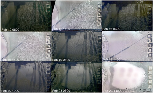
Figure 3. Examples of surface pictures during the experiment. (a) February 12 10:00, Frost flower coverage, (b) February 16 07:00 frost flower coverage, (c) February 19, 15:00 snow-covered frost flowers, and (d) February 23, 15:00 snow-covered sea ice.

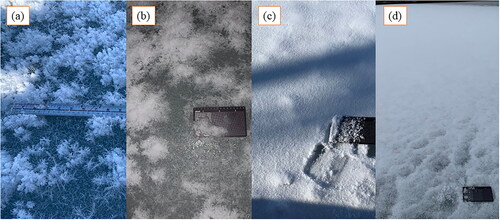
Figure 2 shows a time-series evolution of the snow and sea ice thickness in a sketch format. Sampling events (16 in total) are indicated using blue arrows. In the first phase of the experiment, we started with FF coverage and observed natural temperature and radiation diurnal variations. A site picture is given in Figure 3a for February 12, which shows the FF coverage and the bare sea ice between them. Figure 3b shows the FFs four days later, on February 16. The FFs exhibit some changes in physical structure, as the fragile crystals amalgamated and coalesced. Typically, we expect natural snow to fall throughout the month of February in Winnipeg, but in this particular year, precipitation was very low. To induce a change and examine the impact of adding snow, on February 18 we used a snow-making machine to add snow, resulting in a combined layer of FF and snow that was 1 cm thick. Figure 3c shows the SERF pool surface on February 19. At this point, a continuous layer of snow was distributed across the surface, and the bare sea ice surface could no longer be seen. Trace amounts of natural snow also fell on February 18. The third phase began on February 19, when we added another layer of snow, creating a coverage layer that was 4 cm thick. Snow-covered sea ice on February 23 is shown in Figure 3d. The FF is no longer observable on the ice surface, as they have been completely incorporated into the snowpack.

Meteorological conditions

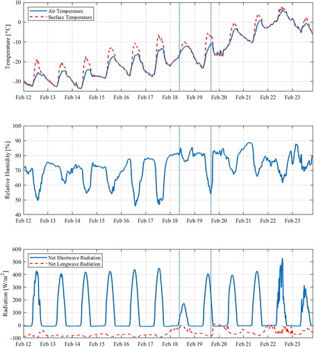
Meteorological conditions for the complete experiment are shown in Figure 4. We note that sunrise was nominally 07:50 and sunset was 17:50 throughout the experiment. The sky was clear throughout the experiment, except for February 18, when some cloud cover occluded the sky. Air temperatures were cold (−30 °C) at the start of the experiment but rose to a peak of +5 °C toward the end of the experiment. There is a clear diurnal cycle in air temperatures of ∼10 °C each day. Surface temperatures were equal to the air temperature over night, but were ∼1–5 °C warmer than air temperature during the day. Relative humidity shows a strong diurnal variation with a minimum at night and peak during the day, except for February 18 when no diurnal cycle is evident. Net shortwave radiation also exhibits a clear diurnal cycle with daily peaks around 400 W/m² and values of 0 during the long nights. Net longwave radiation shows no diurnal cycle and varies from a minimum of −100 W/m² to slightly positive in a few instances.

Figure 4. Automated meteorological data. Top panel: Air and surface temperature. Middle panel: Relative humidity. Bottom panel: Net shortwave and longwave radiation.

Scatterometer data

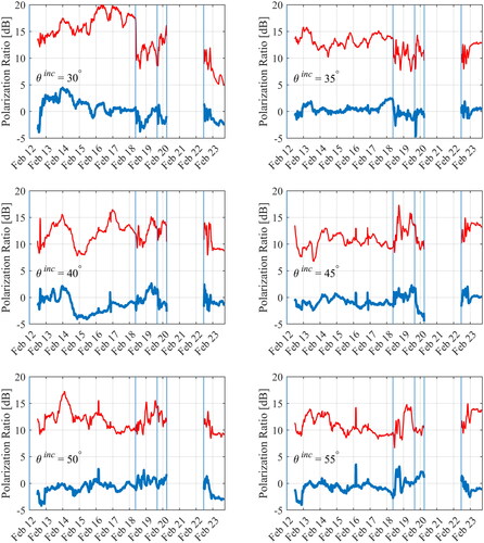
The scatterometers were configured as described in the methods, and data collection began at 09:00 on February 12. C-band NRCS measurements are presented in Figure 6 and Ku-band measurements are shown in Figure 8. Each panel shows the radar elevation incidence angle, with θ^inc ranging from 30° to 55°. In both figures, the solid thick blue line shows σ_VV, dashed red line shows σ_HH (collectively known as co-polarized signals, and abbreviated here as VV and HH), and thick black line shows σ_HV (cross-polarized signal, abbreviated here as HV). The cross-polarized signal, HV, was calculated as the average of HV and VH, based on the assumed reciprocity of the sea ice surface. In post-processing, we checked the similarity between the channels for each instrument and each incidence angle and determined that the error in this assumption was <0.2 dB for C-band and <0.3 dB for Ku-band. Solid vertical blue lines indicate the beginning of phase 2 and phase 3, coinciding with the two snowfall events.

For C-band, initial backscatter levels were low and VV was significantly larger than HH. The initial addition of snow in February resulted in an increase of NRCS for all polarizations. The difference between VV and HH decreased to near zero. NRCS gradually decreased after the snow event. The second snow event on February 19 resulted in a second spike of backscatter increase for lower incidence angles (≤45°), while higher incidence angles maintained a relatively similar NRCS. With continued increase in air temperature and diurnal variations, the snow cover physical state changed and this was observed in the time-series radar data. Notably, on February 22, when air and surface temperatures rose above 0 °C, the HH signal dramatically increased, while VV and VH decreased. These rates were dependent upon the incidence angle of observation.

For Ku-band, initial backscatter levels showed that VV was similar to HH (with some exceptions to be discussed in the next section), and VH was significantly lower. Diurnal variations were apparent, especially at low incidence angles (≤35°). Like C-band, the initial addition of snow on February 18 resulted in an increase of NRCS for all polarizations. The difference between VV and HH remained near zero. NRCS gradually decreased after the snow event. The second snow event on February 19 resulted in another spike increase in backscatter for lower incidence angles (≤45°), while higher incidence angles maintained a relatively similar NRCS. Unfortunately, due to an apparent electrical brown-out, the C-band instrument did not collect accurate HH data from February 20 at 06:30 to the experiment end, and the Ku-band instrument did not collect data between February 20 at 06:30 and February 22 at 11:06 (when it was reset). Notably, on February 22, when air and surface temperatures went above 0 °C, the NRCS exhibited a local minimum and gradually increased to a plateau once the temperatures returned to below zero.

Drone and terrestrial LiDAR data

Drone flights with optical and thermal sensors were conducted, following the schedule in Table 2. Figure 10 shows a time series evolution of the RGB imagery from the drone. The first four panels show the distribution of the FF across the surface of the sea ice. Areas of bare ice can be seen between the FF. Imagery from February 19 shows how the snow completely covered the FF and the sea ice. The FF can still be observed as raised areas on February 19 06:00 and 14:00. After the second snow event, the FF were completely obscured, as shown in the February 19 19:00 panel. The images from February 23 show how the snow cover areal extent retreated and surface changed, due to the air temperature rising above 0 °C.

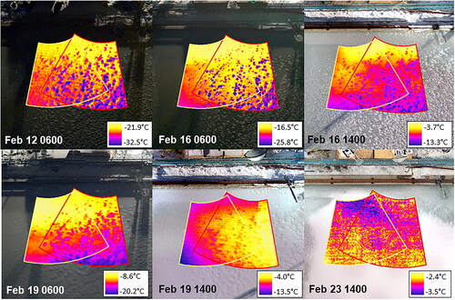
A time series evolution of thermal scanner imagery is presented in Figure 11. On February 12 and 16, the FF are clearly visible as cold regions relative to the bare sea ice on which they reside. February 16 at 14:00 shows a warmer temperature than the previous two panels, owing to the increased air and surface temperatures. The images for February 19 were taken in Phase 2, after the first snow event. The FF can still be seen as relatively cold regions, but a smoothing effect has taken place. For Phase 3, we have one image from February 23, which shows a near uniform temperature distribution across the snow-covered sea ice. At this time, the air temperature was above zero.

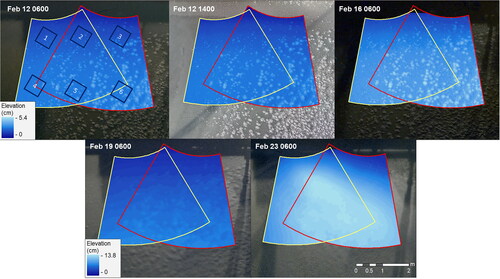
Terrestrial LiDAR scans were performed for five days throughout the experiment. Figure 12 shows the time-series evolution of the elevation profiles, with the scan region for the C-band and Ku-band scatterometers traced out. The upper three panels show the profiles from experiment Phase 1, with FF coverage. The elevation scale was changed for the bottom two panels, which show the results from Phase 2 (bottom left: snow-covered FF) and phase 3 (bottom right: snow cover). The root mean square (RMS) heights that were derived from the LiDAR scans are provided in Table 3. We note that the values for regions 1, 2, and 3 on February 19 and 23 are large, and this was attributed to the local slopes observed within the regions at those times.

Table 3. Root mean square heights (cm) derived from LiDAR scans.

Region	February 12	February 12	February 16	February 19	February 23
	06:00	14:00	06:00	06:00	06:00
1	0.66	0.58	0.92	2.01	2.26
2	0.71	0.64	0.93	1.92	1.86
3	0.80	0.75	1.00	1.93	5.29
4	0.24	0.27	0.28	0.55	1.70
5	0.33	0.32	0.41	0.80	0.60
6	0.35	0.30	0.42	0.61	0.92

Phase 1: Frost flowers on sea ice

The first phase of this experiment started from the initial measurement on February 12 and ended just before we first introduced a layer of snow onto the sea ice on February 18. Initial temperatures were cold and exhibited a diurnal variation (Figure 4). For the first three days (February 12, 13, and 14), the nighttime lows were near −34 °C, with day-time highs reaching −25 °C. The next three days (February 15, 16, and 17) were warmer, with nighttime lows near −25 °C and day-time highs trending from −17 °C to −14 °C.

FF covered the surface of the sea ice, and their height was 1.5 ± 0.5 cm. Measurements on a snow grid plate showed that the grains were 8 mm long and 1 mm wide. We sampled the FF surface for moisture using a Kimwipe and determined that no liquid content was present since we did not observe moisture wicking into the tissue. This was consistent throughout the phase. The mean FF salinity on February 12 was 49.0 ppt, based on eight samples Figure 5. Surface salinity, obtained from scrapings beneath the FF, was 45.5 ppt, based on 10 samples. On February 16, the salinity of the FF was slightly lower, at 37.1 ppt, while surface salinity was 36.2 ppt. We observed that the FF salinity was greater than the surface ice salinity, except at the 10:00 sampling time when the surface ice salinity was greater than the FF. This coincides with the diurnal air and surface temperature increase. After solar noon (12:40), the FF salinity was once again greater than the surface ice.

Figure 5. Time-series salinity evolution of bulk sea ice, sea ice surface, and surface features (FF and snow). Vertical bars indicate the timing of snow addition events.

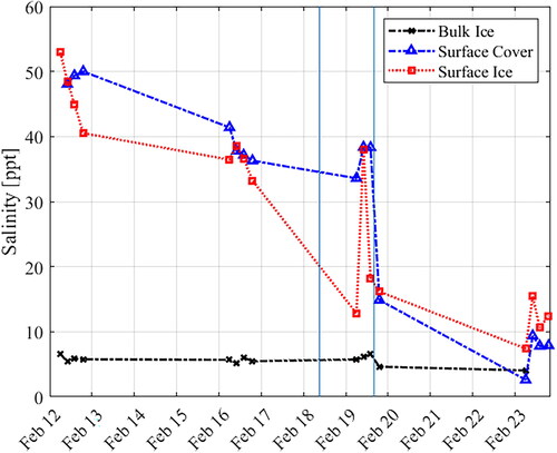
Sea ice thickness increased from 27.5 cm (n = 4) on February 12 to 38.6 cm (n = 4) on February 16. Salinity profiles followed the typical C-shaped curve, with a bulk salinity of 6.0 ppt on February 12 and 5.6 ppt on February 16 (Figure 5).

Drone imagery showed that FF coverage increased in the scatterometer field of view from 15% to 32% between February 12 and February 16. An advantage of the drone data collection was that we were able to able to observe and characterize the FF coverage and rate of change. The top-down imagery gave a clear picture of the distribution across the sea ice surface, which could not be obtained with oblique pictures taken from the side of the SERF pool.

Drone thermal imagery showed that FF areas were colder than areas with a bare ice surface, having the following average difference; 6.5 °C on February 12 at 06:00, 4.8 °C on February 16 at 06:00, and 3.1 °C on February 16 at 14:00 (Figure 11). Acquiring this information was a significant improvement in the thermal characterization of the surface versus hand-held temperature probes. The drone imagery provided a georectified top-down view of the region and we could get results from the middle of the scan regions, without disturbing the site through physical interaction.

LiDAR measurements (Figure 12; Table 3) show that the surface is rough for both C-band and Ku-band based on the Fraunhofer criterion, with the higher frequency seeing a much rougher surface. The minimum RMS height was 0.24 cm. The Fraunhofer criterion requires the average roughness to be greater than λ/32 for a surface to be considered rough, i.e., ks > 0.2, where k = 2π/λ and s is the RMS height. For C-band (5.5 GHz, λ = 5.454 cm), the minimum value of ks is 0.276, and for Ku-band (17.2 GHz, λ = 1.744 cm), the minimum value is 0.867. All values in Table 3 are larger than these values, and therefore the surface is considered to be electromagnetically rough. The roughness profile had a greater RMS height for low incidence angles (regions 1, 2, 3) than high incidence angles (regions 4, 5, 6), by a factor of ∼2. Results showed a slight increase for low incidence angles (regions 1, 2, 3), while it remains relatively constant for higher incidence angles (regions 4, 5, 6). Simultaneously, there was an increase in FF areal coverage (spreading) in the region. This information helps quantify the difference in backscatter level at lower incidence angle versus higher incidence angles.

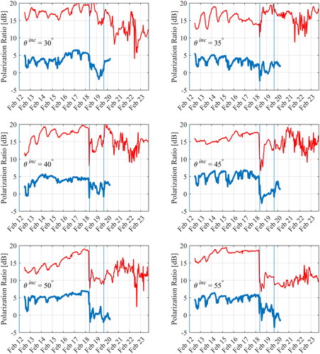
During the first phase, the measurements for C-band VV, HV, and HH were relatively stable (Figure 6). Diurnal variations, which appear as ripples, can readily be seen on the time-series measurements (particularly at θ^inc = 30° and 35° for VV, 35° and 45° for HH, and 35°, 40°, and 45° for HV). These follow the temperature measurements, with maximums occurring in mid-afternoon. We observed that VV > HH and in all cases, the cross-pol, HV, was significantly lower than co-pol (VV and HH). C-band co-polarization ratios (VV/HH) and cross-polarization ratios (VV/HV) are presented in Figure 7. The co-polarization ratio was positive, with a value ranging from 0 to 5 dB. Cross-polarization ratios demonstrated that VV was greater than HV by between 15 dB to 20 dB for the majority of the phase.

Figure 6. C-band scatterometer data. Solid blue lines: VV, dashed red lines: HH, thick black lines: HV.

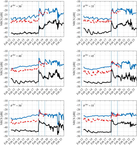
Figure 7. C-band scatterometer polarization ratios. Solid blue lines: VV/HH, dashed red lines: VV/HV.

For Ku-band, the measurements had a gradual increasing trend for incidence angles >30° (Figure 8). For this frequency, we note that VV ∼= HH, except for a portion of the time-series plot at 40° incidence angle (February 14–16), where HH > VV by a few dB. In all cases, the cross-polarization was significantly lower than that co-pol (VV and HH) by 10 dB or more. Diurnal variations can readily be seen on all the time-series measurements for all polarizations, with the greatest daily variability appearing at low incidence angles (i.e., 30°). Ku-band co-polarization ratios (VV/HH) and cross-polarization ratios (VV/HV) are presented in Figure 9. The co-polarization ratio was between −4 and 0 dB (negative) for the first 12 hours of the experiment. Afterward, there were, low incidence angles (30° and 35°) showed a positive value and settled to ∼0 dB near the end of the phase. The 40° incidence angle started near 0 dB and decreased to ∼4 dB until it gradually increased back up to 0 dB over several days. Mid-to high incidence angles (45° to 55°) hovered around 0 dB. Cross-polarization ratios demonstrated that VV was greater than HV by between 12 dB to 20 dB (30°). For the other incidence angles, the cross-polarization ratio ranged between 8 dB and 16 dB, with the largest variations being seen for 40° incidence angle.

Figure 8. Ku-band scatterometer data. Thick blue lines: VV, thin red lines: HH, thick black lines: HV.

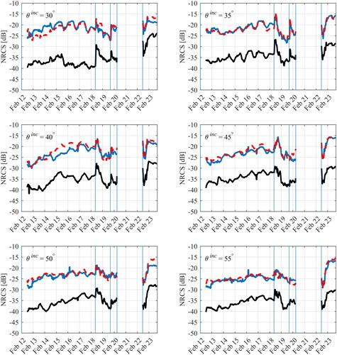
Figure 9. Ku-band scatterometer polarization ratios. Thick blue lines: VV/HH, thin red lines: VV/HV.

Phase 2: Snow-covered frost flowers on sea ice

The second phase of this experiment started from when we introduced a layer of snow on the sea ice on February 18 from ∼10:00 to 16:00 and ended when we added a second layer of snow on February 19 (16:00). We added 1 cm of snow using a snow making machine and simultaneously, a trace amount of natural snow fell onto the frost-flower-covered sea ice on February 18.

Temperatures were warmer than in the first phase and exhibited a diurnal variation, with a nighttime low near −23 °C, and day-time highs reaching −12 °C (Figure 4). Humidity remained high during the day on February 18 and cloud cover reduced the net shortwave radiation.

The addition of the snow resulted in a compaction and combination of snow and FF. The total thickness was 1 cm once the areas between, and on, the FF structures were filled in with snow. Measurements on a snow grid plate showed that the grains were 1 mm in diameter, with a powdery consistency. We sampled the snow surface (i.e., the air/snow interface) for moisture using a Kimwipe and determined that no liquid content was present since we did not observe moisture wicking into the tissue. This was consistent throughout the phase. However, the basal layer of the snow had a powdery moist consistency at 14:00 and the ice surface (below the snow) exhibited wetness detectable by a Kimwipe. This is depicted in Figure 2.

The time-series salinities are plotted in Figure 5, where the surface cover is snow on February 19. The mean snow salinity on February 19 was 36.8 ppt, based on nine samples. Surface salinity, obtained from scrapings beneath the snow was 23.0 ppt, based on three samples.

Sea ice thickness was 46.2 cm (n = 3) on February 19. Salinity profiles followed the typical C-shaped curve, with a bulk salinity of 6.1 ppt.

Drone measurements showed that the FF was visibly present under the layer of snow. RGB imagery showed that areas with FF were elevated under the snow (Figure 10). The georectified, top-down view of the snow-covered FF from the drone indicated that the snow cover was distributed equally over scatterometer footprint region, which was used to interpret the NRCS results.

Figure 10. Time-series evolution of surface conditions obtained from drone RGB images.

Thermal imagery revealed that FF areas remained colder than the surrounding smooth ice area, though these areas become less distinct under the snow layer (Figure 11). Even with snow cover, FF areas are 4.7 °C colder than the surrounding ice area for February 19 at 06:00, and 1.0 °C colder for February 19 at 14:00. A temperature gradient was observed across the scan region, with the temperatures at low incidence angles (nearest to the pool edge) being warmer than the higher incidence angles.

Figure 11. Drone thermal imagery displayed for the Ku-band (yellow) and C-band (red) footprints.

After the addition of snow, the measurements for C-band VV, HV, and HH showed a large transient increase (on average 10.6 dB), followed by a decrease (on average 8.5 dB) (Figure 6). VV now became approximately equal to HH, giving a co-polarization ratio of <3 dB (Figure 7). The ratio between VV and HV showed a rapid decrease of 10 dB for incidence angles ≥40° (Figure 7). NRCS levels were consistently higher than in the previous phase, indicating the major backscatter influence that the snow cover created.

Ku-band measurements for VV, HV, and HH showed a large transient increase (on average 5.5 dB) (Figure 8). This was followed by a decrease (on average 8.5 dB) to levels that were akin to the beginning of the experiment. VV was approximately equal to HH, similar to Phase 1, giving a co-polarization ratio of <3 dB (Figure 7). The ratio between VV and HV showed a rapid decrease of 10 dB for 30° incidence angle, but for other incidence angles, it remained similar to Phase 1 values (between 8 and 16 dB).

Phase 3: Thin snow cover on sea ice

The third phase of this experiment started when we introduced another layer of snow on the sea ice on February 19 (from 16:00 to 19:00) using a snow making machine. This phase ended on February 23, with the conclusion of the experiment.

The air temperature had a strong warming trend through this phase, with a minimum of −16 °C overnight on February 19 to a daytime maximum of +6 °C on February 22 (Figure 4). Shortwave radiation followed a diurnal cycle and humidity ranged between 60% and 90%.

After the snow had been added, we performed physical sampling measurements. A site picture is provided in Figure 3c for February 19 at 19:00. We sampled the snow surface (i.e., the air/snow interface) for moisture using a Kimwipe and determined that no liquid content was present, as we did not observe moisture wicking into the tissue; however, the snow/ice interface had water in the liquid phase. The snow itself had a perceptible wetness, as the grains adhered to each other and had the powdery, wet consistency. Initial measurements on a snow grid plate on February 19 showed 1 mm, round fine snow grains. The mean snow salinity on February 19 was 36.8 ppt, based on nine samples (Figure 5). Surface salinity, obtained from scrapings beneath the snow was 23.0 ppt, based on three samples.

We returned for a final series of four sampling events on February 23. The surface had changed, due to warm temperatures and melting surface. A site picture is provided in Figure 3d for February 23 at 15:00. At this time, the snow thickness had decreased to 3 cm and measurements on a snow grid plate showed that the grain structures were 2 mm with 8 mm aggregate pellets. Surface ice salinity had decreased to around 12 ppt on average, while the snow salinity was <10 ppt (see Figure 5).

Sea ice thickness was stable, from 47 cm (n = 2) on February 19 and 47 cm (n = 1) on February 23. Salinity profiles followed the typical C-shaped curve, with a bulk salinity of 5.8 ppt on February 19 and 4.1 ppt on February 23.

RGB drone imagery showed that snow cover was distributed across the full ice surface on February 19 at 19:00 and retreated to the center of the ice surface between February 19 and 23 (Figure 10).

Thermal drone imagery showed that the snow surface had a near-uniform temperature distribution within the scatterometer footprint during this phase of the experiment (Figure 11). This meant that during this phase, the approach of using a handheld temperature probe to characterize the snow surface temperature at several discrete points was an effective representation of the entire surface temperature within the scatterometer scan region.

For C-band scatterometer measurements, the addition of the snow created an increase in backscatter at low to midrange incidence angles (θ^inc ≤ 40°) (on average ∼3 dB) (Figure 6). Unlike the first snow event in phase 2, the scattering trend did not have a transient increase followed by a decrease. At higher angles, a change in NRCS due to snow addition was not readily detectable. Co-polarization ratios showed an increase of ∼3 dB for 30°–45°, but it was fairly constant for higher angles (Figure 7). Cross-polarization ratios showed an increase for 30° and 40°, while for other angles, it remained fairly constant.

For Ku-band scatterometer measurements, similar to C-band, the addition of the snow created an increase in backscatter at low to midrange incidence angles (θ^inc ≤ 40°) (on average 6.7 dB) (Figure 8). Unlike the first snow event in phase 2, the scattering trend did not have an overall transient increase followed by a decrease. The exception is for 35°, which showed a 10 dB increase, followed by an 8 dB decrease for VV and HH, with a smaller peak exhibited by VH. The exact reason for the larger transients at 35° is not known, and future experimental/modeling studies should be performed to help elucidate the mechanism. Co-polarization ratios showed fairly constant values, with the largest change being seen at 45° (Figure 9). Cross-polarization ratios remained between 8 and 16 dB.

For the remainder of the experiment, on February 22 and 23, we noted that the backscatter had a transient increase that followed the trend of when the air and surface temperatures returned to below 0 °C. VV and HH were nearly the same and HV was around 10 dB lower. From this dataset, the Ku-band NRCS trend follows the temperature variation, and more directly, the temperature/liquid water content in the upper level of the snow. In physical sampling, we noted that the snow/ice interface had liquid content, but the snow surface was dry.

Discussion

The previous section presents new experimental measurement results for C-band and Ku-band scattering responses of a thin FYI surface. The experiment was partitioned into three separate phases, based on the frost flower and snow coverage. Detailed information on the temporal evolution of the sea ice physical and thermodynamic properties were provided. Furthermore, drone imagery and terrestrial LiDAR data were collected to give additional characterization beyond traditional physical sampling. In this section, we evaluate the temporal evolution of the scattering responses, in connection with the snow and ice properties. We assess how the physical and thermodynamic properties give rise to the C- and Ku-band scattering response and evaluate how multi-sensor fusion can improve our understanding of these linkages within snow-covered sea ice.

Phase 1: Frost flowers on sea ice

The experiment began with the presence of FF-covered sea ice. FF forms under specific conditions of low temperatures, high humidity, and low wind speed. Style and Worster discussed their formation mechanisms in detail (Style and Worster 2009) and draw attention to the short-lived transient nature of these features, which typically form on very young sea ice but are quickly covered by snow or destroyed by wind ablation. In our own field observations, we have encountered fields of FF on sea ice that were similar in thickness to this experiment (Isleifson et al. 2010).

Measured FF salinities are similar to those previously measured SERF (e.g., peak values of ∼51 PSU, reported by Isleifson et al. 2014) and field measurements (21.5–62.5 PSU), but on the low side when compared to other studies (e.g., Martin et al. 1995 reported 52–107 PSU for FF).

As mentioned earlier, the ice surface salinity was greater than the FF salinity, which coincided with the air and surface temperature increases. This was also observed in previous studies at SERF (Isleifson et al. 2014). The FF has an insulating effect, with temperatures below the FF being warmer than neighboring bare ice. As pointed out by Barber et al. (1998), the brine volumes in basal layers of snow respond to the atmospheric forcings. Similarly, the thermodynamic effects in this situation are playing a role in the salinity profiles. The regions of bare sea ice near the edge of the pool were warmer than the tops of the FF, as can be seen in the thermal imagery (Figure 11). This temperature gradient is attributed to the non-uniform distribution of the FFs, where a greater portion of the surface near the edge of the pool had sparse FF coverage.

In comparison with literature data, the polarimetric scattering measurements had backscatter levels similar to newly-formed sea ice. For example, in a study of FF covered sea ice, Isleifson et al. (2014) reported VV, HH, and HV values of −28, −30, and −36 dB at 35° incidence for dry FF conditions with thin sea ice.

The NRCS remained relatively low and constant throughout this phase and the variations were based on thermodynamic changes in the FF and surface temperature diurnal temperature cycling. With temperature increases, it is postulated that the effect is to increase effective roughness at the interface of the FF and sea ice. This has been described as a thermodynamic effect in brine rich snow basal layers (Barber et al. 1998), and with the greater salinity of FF, the impact is readily observed as a backscatter increase associated with temperature rise. This is consistent with other studies on the diurnal thermal variations on backscattering over sea ice. For example, in their study of thin sea ice, Nghiem et al. (1998) found that the backscatter and temperature cycles are correlated and have a synchronous behavior.

The penetration depth of microwaves into snow-covered sea ice is governed by the frequency and consequently, we expect that there would be very little penetration into the sea ice due to the high sea ice surface salinity. We consider that the backscatter was primarily driven by the surface features (i.e., FF surface) and/or the sea ice surface ice. This assertion agrees with other modeling studies, who have also found that cross-pol is very low and often near the instrument noise floor for rough interface scattering (Komarov et al. 2015). For comparison, in our experiment, the cross-polarized C-band backscatter is around −45 dB (noise floor is −56 dB), and Ku-band is around −40 dB (noise floor is −42 dB).

From these analyses, we conclude that the backscattering from the FF covered surface is driven by the FF and highly saline sea ice surface. This makes sense, given that the salinity of the sea ice surface is very high, and the temperature variation is known to be a factor in backscattering measurements (Barber and Nghiem 1999; Yackel et al. 2017). Moreover, the Ku-band results exhibit a greater fluctuation with the diurnal temperature variation than the C-band results. The FF had a non-uniform distribution across the scatterometer field of view. Horizontal development was observed in this experiment, as in other FF experiments. For Ku-band HH signals were sometimes greater than VV at mid-range angles (40° and 45°) and we attribute this to the non-uniformity. Therefore, to have greater information on how the surface coverage responds to meteorological forcings, one should utilize a higher frequency system (i.e., choose the Ku-band system over the C-band system when we want to focus on the upper layer, such as FF coverage). The drone and LiDAR data provided additional key information on the physical and thermodynamic state of the sea ice in the scatterometer field of view.

Phase 2: Snow-covered frost flowers on sea ice

At the beginning of this phase, we added snow onto the FF covered sea ice surface. This would be a common event in the natural Arctic environment in the winter season. In our experiment, we originally expected that natural snow would have fallen onto the surface, but this year had particularly low snowfall amounts in Winnipeg. One of the advantages of our SERF mesocosm is that we can introduce changes through using a snow making machine.

Detailed characterization of snow and ice salinities is given in Figure 5. Similar to earlier in the experiment, we observed that the surface cover salinity was greater than the surface ice salinity, except at the 10:00 sampling time, where this relationship inverted (i.e., the surface ice salinity was greater than the snow). This suggests that brine was migrating down onto the sea ice surface and then wicked back up into the surface coverage. Similar observations of brine wicking from underlying sea ice into snow cover has been reported by Barber et al. (1995) and Barber and Nghiem (1999).

Calculations from the LiDAR data showed that the surface is rough for both C-band and Ku-band based on the Fraunhofer criterion (Table 3; Figure 12). RMS values had approximately doubled from before the addition of the snow. The snow was not perfectly uniformly distributed across the sea ice surface, with a slight increase in elevation, leading from the pool edge toward the middle. Areas of snow-covered FF were seen to protrude from the snow mean level. The roughness profile had a greater RMS height for low incidence angles (regions 1, 2, 3) than high incidence angles (regions 4, 5, 6), by a factor of ∼3.

Figure 12. LiDAR scan data, displayed for the Ku-band (yellow) and C-band (red) footprints. Subsets used for RMS calculation are shown in the top left panel, corresponding to Table 3. Note that the pool edge is at the top of the images.

The C-band measurements showed a significant increase in backscatter (Figure 6). The large increase in backscatter makes sense because the added snow was wet, and this increased the dielectric contrast (Komarov et al. 2015). Adding dry snow would not affect the backscatter at C-band (Bernier and Fortin 1998). This is because the C-band wavelength was 5.45 cm and typically elements that are 1/10 of a wavelength are considered to be appreciable scatterers. Cross-polarization was strongly affected, indicating a volumetric scattering component from the snow. Drone imagery indicated that snow-covered FF protruded from the surface and their temperatures were colder than the surrounding snow surface. This variation potentially contributes to the radar wave depolarization and hence the cross-polarized return. As time progressed, the temperature exhibited a diurnal minimum and the backscatter decreased. While VV remained greater than HH, and cross-polarization (HV) followed the co-polarization trend, signifying a reduction in volume scattering and indicating that the scattering contributions were strongly from interface roughness.

The Ku-band measurements showed a large increase in backscatter levels. This trend is similar to what was seen in Lytle et al. (1993). Ku-band had a smaller increase than C-band and was less sensitive to the addition of snow to the FF covered ice surface. While surface roughness increased, it is clear that the addition of snow cover had a greater effect on the C-band backscatter. Ku-band would be sensitive to the snow, as the Ku-band wavelength was 1.74 cm and snow grain sizes were ∼1 mm and are therefore appreciable scatterers (Drinkwater et al. 1992). However, the transition to snow-covered sea ice had a much larger effect on the C-band NRCS measurements. On average for all incidence angles, the VV, HH, and HV increased by 8.7 dB, 11.6 dB, and 12.6 dB, respectively. It also had a greater effect on the co-polarization and cross-polarization ratios. From these analyses, we conclude that C-band is the better candidate for monitoring the transition from a surface with sparse FF coverage to a snow-covered FF first year ice. The drone and LiDAR data enhanced our information on the physical profile and the relative thermodynamic state of the snow-covered FF.

Phase 3: Thin snow cover on sea ice

To begin this phase, we added another layer of snow onto the snow-covered sea ice surface. Characterization of snow and ice salinities are shown in Figure 5 and within the ranges reported within the literature (e.g., ranging from 1 to 20 ppt, as reported by Komarov et al. 2015 for 4 cm of snow on sea ice, Nandan et al. 2016, and Crocker 1992). Salinity in the basal layer of the snow impacts the dielectric constant and the higher loss leads to attenuation. Toward the end of the experiment, the surface salinity was greater than the overlying snow cover, which is typically expected.

As before, calculations show that the surface is rough for both C-band and Ku-band based on the Fraunhofer criterion (Table 3; Figure 12). After the melting events, due to warm air and surface temperatures, the snow was not uniformly distributed across the sea ice surface. Within the radar footprint, the roughness profile for regions 1, 2, 5, and 6 showed some change, but it was not as substantial as the differences seen in regions 3 and 4. Region 3 shows an RMS height of 5 cm, but that is evidently influenced by the local slope that can be observed in Figure 12.

The snow cover area decreased due to two factors. Firstly, the distribution of the snow across the pool surface was not perfectly uniform. The snowfall came from a snow making machine, meaning that despite best efforts, the distribution of the induced precipitation will not be equal across the entire pool surface. Furthermore, the initial surface had FF coverage and they were not randomly distributed across the surface. Secondly, the sides of the pool are constructed with concrete. Since concrete has a lower specific heat than snow and sea ice, it heats up faster and this results in faster melt rates at the edge of the pool surface when the air temperature is above 0 °C.

After the initial transient, the time-series NRCS showed some ripple, presumably due to the temperature fluctuations (and hence, the snow liquid water content). The NRCS levels are similar to what has been reported in field studies with snow cover on thin FYI (e.g., Isleifson et al. 2010).

At the peak temperatures, on February 22, we observed a decrease in VV and HV. This was ascribed to the rapid change in the snow cover, as the melt progressed, and liquid water content effects were evident. In other words, the dielectric loss reduced the backscatter from the wet snow.

The increase in backscatter at Ku-band, due to the snow addition, has been observed by others in the field (Yueh et al. 2009; King et al. 2013; Lytle et al. 1993; Gunn et al. 2015). At higher angles, the increase was not large (a few dB, at most). Unfortunately, the instrument had a malfunction and did not collect data between February 20 at 06:30 and February 22 at 11:06, so there was a gap in the time-series data.

The results of Phase 3 indicate that both C-band and Ku-band have complementary behaviors that can be used together to monitor snow events, with warming and cooling trends. Ku-band scatterometer results, especially at lower incidence angles, showed the greatest sensitivity to the addition of snow. Later, when the air temperature increased to several degrees above 0 °C, the C-band instrument was highly sensitive to the change of water in liquid content. After the temperature reached its peak and then began to cool below freezing, the Ku-band had a notable transient increase. C-band showed changes too, but they were more complex than the Ku-band results, which had a clear transient signal for all incidence angles. The third phase was complex, with multiple factors simultaneously affecting the microwave scattering behavior. Our approach of using multiple sensors, both surface and drone-based, enhanced the characterization of the physical and thermodynamic state, which assisted in interpreting the measured scatterometer data.

Conclusion

The results of this experimental study on thin FYI with FF and snow cover help to address gaps in our knowledge of the heat flux between the ocean, ice, and atmosphere during the freeze-up and early winter seasons. We have presented a case study, in which we measured and evaluated the temporal evolution of C-band and Ku-band scattering responses of a thin FYI surface for a variety of surface features (e.g., FF and snow).

We divided our experimental analysis into three main phases, based on the physical state of the sea ice surface (specifically, phases were divided by snowfall events). We examined the link between the temporally evolving sea ice, FF, and snow physical properties and the measured scattering response. Throughout the analyses, we focused on assessing how multi-sensor fusion, through the use of drone imagery, terrestrial LiDAR, and surface-based scatterometers, could enhance our understanding of the snow-covered sea ice system.

On an individual basis, each of the instruments used in this experiment could provide a characterization of the properties of thin FYI that we observed in the SERF pool. Further analysis on each of the sensor data could be performed in future studies, such as investigating the polarimetric parameters of the scatterometers, surface characterization from the LiDAR, or addressing microwave interactions with electromagnetic modeling. Combining the sensors provided complementary datasets and enhanced our overall characterization of the sea ice; however, it is challenging to use and integrate the data from multiple sensors, as each instrument requires expertise in operation and processing.

With regard to the main objectives of the experiment, here is a summary of our findings:

The temporal evolution of C-band scattering responses was measured and presented. In Phase 1, with FF coverage, the backscatter was relatively low in magnitude, and a diurnal variation that coincided with daily temperature variations was observed (primarily for low incidence angles). In Phase 2, with the addition of snow, we observed an immediate large backscatter increase for all polarizations, followed by a gradual decrease. In Phase 3, another layer of snow was added. A distinct NRCS increase was seen for incidence angles up to 45°, but it was not as apparent for 50° and 55°. Toward the experiment end, the backscatter showed a major decrease when the air temperatures rose well above 0 °C and snow melt occurred. After that point, the backscatter showed some variability, as temperatures fluctuated about the freezing point.

The temporal evolution of Ku-band scattering responses was measured and presented. Relatively speaking, the Ku-band backscatter was higher in magnitude than C-band. In Phase 1, the backscatter had a relatively low magnitude and a diurnal variation that was similar to C-band. The addition of snow in Phase 2 resulted in an immediate large backscatter increase for all polarizations, followed by a gradual decrease. In Phase 3, an immediate backscatter increase due to snow was observed as some angles (particularly 35°), but for most angles, it did not substantially change. Further investigation into this phenomenon is needed. Similar to C-band, toward the end of the experiment, the backscatter was low when the air temperatures rose well above 0 °C and snow melt occurred. After that point, the backscatter increased and was much more stable than C-band.

We assessed how multi-sensor fusion, through the use of drone imagery, terrestrial LiDAR, and surface-based scatterometers, can complement and enhance our understanding of the snow-covered sea ice system. Drones give a top-down view, which can aid in regional classification purposes. The data are georectified, meaning that orientation and distances are characterized. While seemingly obvious, it is important to have such imagery, as it gives a complementary view on the evolution of the surface, which cannot be observed from oblique views. For instance, a top down view gives a better perspective for estimating frost flower coverage.

Drone-based TIR sensors can be used to show the temperature distributions, which affect the microwave backscatter. These results can be distilled down to the individual scan region and/or incidence angle, to give high fidelity characterization. The results of this study highlighted the potential variability of surface temperatures, even within one footprint, due to varying surface features.

Surface-based LiDAR can be used to create a map of the region and with appropriate processing, the surface roughness statistics can be derived. We can rectify the LiDAR, thermal, and RBG to a common projection, which permits intercomparison of the radar field of view and surface roughness.

Understanding the temporal evolution of multifrequency scattering processes of sea ice is critical for accurately observing, predicting, and modeling the thermodynamic behavior of sea ice, as well as its impacts on the global climate. This study demonstrated a new sensor fusion approach that enhanced the measurement and characterization of snow-covered sea ice physical and thermodynamic properties. These results can be used to improve our understanding of the microwave interactions at multiple frequencies, such that satellite remote sensing products can be better linked to the rapidly changing sea ice in the cryosphere.

Acknowledgments

The authors would like to acknowledge the leadership and scientific vision of Dr. David Barber. His mentorship has been instrumental in each of the author’s research careers.

We acknowledge the technical support of the SERF Technician, D. Binne.

Disclosure statement

No conflict of interest was reported by the author(s).

Additional information

Funding

D. Isleifson acknowledges support from the Natural Sciences and Engineering Research Council of Canada (NSERC) Discovery Grants Program. D. Babb acknowledges support from NSERC and is supported by the Canada Research Chair Program (D. Barber) and Canada Excellence Research Chair Program (D. Dahl-Jensen).

References

- Alexeev, V.A., Walsh, J.E., Ivanov, V.V., Semenov, V.A., and Smirnov, A.V. 2017. “Warming in the Nordic seas, North Atlantic storms and thinning Arctic sea ice.” Environmental Research Letters, Vol. 12(No. 8): pp. 084011. doi:10.1088/1748-9326/aa7a1d.
- AMAP. 2007. Arctic Oil and Gas. Oslo: Arctic Monitoring and Assessment Programme (AMAP), 40.
- Asihene, E., Desmond, D.S., Harasyn, M.L., Landry, D., Veenaas, C., Mansoori, A., Fuller, M.C., et al. 2022. “Toward the detection of oil spills in newly formed sea ice using C-band multipolarization radar.” IEEE Transactions on Geoscience and Remote Sensing, Vol. 60: pp. 1–15. doi:10.1109/TGRS.2021.3123908.
- Barber, D.G. 2005. “Microwave remote sensing, sea ice and Arctic climate.” Physics in Canada (PiC), Vol. 61: pp. 105–111.
- Barber, D.G., and Nghiem, S.V. 1999. “The role of snow on the thermal dependence of microwave backscatter over sea ice.” Journal of Geophysical Research: Oceans, Vol. 104(No. C11): pp. 25789–25803. doi:10.1029/1999JC900181.
- Barber, D.G., Fung, A.K., Grenfell, T.C., Nghiem, S.V., Onstott, R.G., Lytle, V.I., Perovich, D.K., and Gow, A.J. 1998. “The role of snow on microwave emission and scattering over first-year sea ice.” IEEE Transactions on Geoscience and Remote Sensing, Vol. 36(No. 5): pp. 1750–1763. doi:10.1109/36.718643.
- Barber, D.G., Reddan, S.P., and LeDrew, E.F. 1995. “Statistical analysis of the geophysical and electrical properties of snow on landfast first year sea ice.” Journal of Geophysical Research, Vol. 100(No. C2): pp. 2673–2686. doi:10.1029/94JC02200.
- Beaven, S.G., Gogineni, S.P., Gow, A., Lohanick, A., and Jezek, K. 1993. Radar Backscatter Measurements from Simulated Sea Ice during CRRELEX'90. RSL Technical Report 8243-2.
- Bernier, M., and Fortin, J.-P. 1998. “The potential of times series of C-band SAR data to monitor dry and shallow snow cover.” IEEE Transactions on Geoscience and Remote Sensing, Vol. 36(No. 1): pp. 226–243. doi:10.1109/36.655332.
- Blanchard-Wrigglesworth, E., Farrell, S.L., Newman, T., and Bitz, C.M. 2015. “Snow cover on Arctic sea ice in observations and an Earth System Model.” Geophysical Research Letters, Vol. 42(No. 23): pp. 10–342. doi:10.1002/2015GL066049.
- Bredow, J.W., and Gogineni, S. 1990. “Comparison of measurements and theory for backscatter from bare and snow-covered saline ice.” IEEE Transactions on Geoscience and Remote Sensing, Vol. 28(No. 4): pp. 456–463. doi:10.1109/TGRS.1990.572921.
- Calders, K., Armston, J., Newnham, G., Herold, M., and Goodwin, N. 2014. “Implications of sensor configuration and topography on vertical plant profiles derived from terrestrial LiDAR.” Agricultural and Forest Meteorology, Vol. 194: pp. 104–117. doi:10.1016/j.agrformet.2014.03.022.
- Crocker, G. 1992. “Observations of the snow cover on sea ice in the Gulf of Bothnia.” International Journal of Remote Sensing, Vol. 13(No. 13): pp. 2433–2445. doi:10.1080/01431169208904280.
- Domine, F., Taillandier, A.S., Simpson, W.R., and Severin, K. 2005. “Specific surface area, density and microstructure of frost flowers.” Geophysical Research Letters, Vol. 32(No. 13): pp. 1–4. doi:10.1029/2005GL023245.
- Douglas, T.A., Domine, F., Barret, M., Anastasio, C., Beine, H.J., Bottenheim, J., Grannas, A., et al. 2012. “Frost flowers growing in the Arctic ocean-atmosphere–sea ice–snow interface: 1. Chemical composition.” Journal of Geophysical Research: Atmospheres, Vol. 117(No. D14): pp. 1–15. doi:10.1029/2011JD016460.
- Drinkwater, M.R., Kwok, R., Rignot, E., Israelsson, H., Onstott, R.G., and Winebrenner, D.P. 1992. “Chap. 24. Potential applications of polarimetry to the classification of sea ice.” In Microwave Remote Sensing of Sea Ice, Vol. 68, edited by F.D. Carsey. Washington, D. C.: American Geophysical Union.
- Fofonoff, N.P. 1985. “Physical properties of seawater: A new salinity scale and equation of state for seawater.” Journal of Geophysical Research, Vol. 90(No. C2): pp. 3332–3342. doi:10.1029/JC090iC02p03332.
- Galley, R.J., Else, B.G.T., Geilfus, N.-X., Hare, A.A., Babb, D., Papakyriakou, T., Barber, D.G., and Rysgaard, S. 2015. “Micrometeorological and thermal control of frost flower growth and decay on young sea ice.” Arctic, Vol. 68(No. 1): pp. 79. doi:10.14430/arctic4457.
- Grenfell, T.C., Barber, D.G., Fung, A.K., Gow, A.J., Jezek, K.C., Knapp, E.J., Nghiem, S.V., et al. 1998. “Evolution of electromagnetic signatures of sea ice from initial formation to the establishment of thick first-year ice.” IEEE Transactions on Geoscience and Remote Sensing, Vol. 36(No. 5): pp. 1642–1654. doi:10.1109/36.718636.
- Gunn, G.E., Brogioni, M., Duguay, C., Macelloni, G., Kasurak, A., and King, J. 2015. “Observation and modeling of X-and Ku-band backscatter of snow-covered freshwater lake ice.” IEEE Journal of Selected Topics in Applied Earth Observations and Remote Sensing, Vol. 8(No. 7): pp. 3629–3642. doi:10.1109/JSTARS.2015.2420411.
- Harasyn, M.L., Isleifson, D., Chan, W., and Barber, D.G. 2020. “Multi-scale observations of the co-evolution of sea ice thermophysical properties and microwave brightness temperatures during the summer melt period in Hudson Bay.” Elementa: Science of the Anthropocene, Vol. 8(No. 4): pp. 1–21. doi:10.1525/elementa.412.
- Hudak, A.T., Evans, J.S., Smith, S., and Matthew, A. 2009. “LiDAR utility for natural resource managers.” Remote Sensing, Vol. 1(No. 4): pp. 934–951. doi:10.3390/rs1040934.
- Isenburg, M. 2014. “LAStool – Efficient LiDAR processing software.”
- Isleifson, D., Galley, R.J., Barber, D.G., Landy, J.C., Komarov, A., and Shafai, L. 2014. “A study on the C-band polarimetric scattering and physical characteristics of frost flowers on experimental sea ice.” IEEE Transactions on Geoscience and Remote Sensing, Vol. 52(No. 3): pp. 1787–1798. doi:10.1109/TGRS.2013.2255060.
- Isleifson, D., Galley, R.J., Firoozy, N., Landy, J.C., and Barber, D.G. 2018. “Investigations into frost flower physical characteristics and the C-band scattering response.” Remote Sensing, Vol. 10(No. 7): pp. 991. doi:10.3390/rs10070991.
- Isleifson, D., Hwang, B., Barber, D.G., Scharien, R.K., and Shafai, L. 2010. “C-band polarimetric backscattering signatures of newly formed sea ice during fall freeze-up.” IEEE Transactions on Geoscience and Remote Sensing, Vol. 48(No. 8): pp. 3256–3267. doi:10.1109/TGRS.2010.2043954.
- Isleifson, D., Mead, J.B., Fuller, M.C., Hicks, L., Desmond, D., Asihene, E., Stern, G.A., and Barber, D.G. 2023. “A multi frequency suite of polarimetric scatterometers for arctic remote sensing.” URSI International Symposium on Electromagnetic Theory. Vancouver: IEEE, 4.
- Jenssen, R.O.R., Eckerstorfer, M., and Jacobsen, S. 2020. “Drone-mounted ultrawideband radar for retrieval of snowpack properties.” IEEE Transactions on Instrumentation and Measurement, Vol. 69(No. 1): pp. 221–230. doi:10.1109/TIM.2019.2893043.
- King, J.M.L., Kelly, R., Kasurak, A., Duguay, C., Gunn, G., and Mead, J.B. 2013. “UW-Scat: A ground-based dual-frequency scatterometer for observation of snow properties.” IEEE Geoscience and Remote Sensing Letters, Vol. 10(No. 3): pp. 528–532. doi:10.1109/LGRS.2012.2212177.
- Komarov, A.S., Isleifson, D., Barber, D.G., and Shafai, L. 2015. “Modeling and measurement of C-band radar backscatter from snow-covered first-year sea ice.” IEEE Transactions on Geoscience and Remote Sensing, Vol. 53(No. 7): pp. 4063–4078. doi:10.1109/TGRS.2015.2390192.
- Kwok, R. 2018. “Arctic sea ice thickness, volume, and multiyear ice coverage: Losses and coupled variability (1958–2018).” Environmental Research Letters, Vol. 13(No. 10): pp. 105005. doi:10.1088/1748-9326/aae3ec.
- Landy, J.C., Isleifson, D., Komarov, A.S., and Barber, D.G. 2015. “Parameterization of centimeter-scale sea ice surface roughness using terrestrial LiDAR.” IEEE Transactions on Geoscience and Remote Sensing, Vol. 53(No. 3): pp. 1271–1286. doi:10.1109/TGRS.2014.2336833.
- Landy, J.C., Komarov, A.S., and Barber, D.G. 2015. “Numerical and experimental evaluation of terrestrial LiDAR for parameterizing centimeter-scale sea ice surface roughness.” IEEE Transactions on Geoscience and Remote Sensing, Vol. 53(No. 9): pp. 4887–4898. doi:10.1109/TGRS.2015.2412034.
- Li, J., Schachtman, D.P., Creech, C.F., Wang, L., Ge, Y., and Shi, Y. 2022. “Evaluation of UAV-derived multimodal remote sensing data for biomass prediction and drought tolerance assessment in bioenergy sorghum.” The Crop Journal, Vol. 10(No. 5): pp. 1363–1375. doi:10.1016/j.cj.2022.04.005.
- Lytle, V.I., Jezek, K.C., Hosseinmostafa, A.R., and Gogineni, S.P. 1993. “Laboratory backscatter measurements over urea ice with a snow cover at Ku band.” IEEE Transactions on Geoscience and Remote Sensing, Vol. 31(No. 5): pp. 1009–1016. doi:10.1109/36.263770.
- Martin, S., Drucker, R., and Fort, M. 1995. “A laboratory study of frost flower growth on the surface of young sea ice.” Journal of Geophysical Research, Vol. 100(No. C4): pp. 7027–7036. doi:10.1029/94JC03243.
- Melling, H. 1998. “Detection of features in first-year pack ice by synthetic aperture radar (SAR).” International Journal of Remote Sensing, Vol. 19(No. 6): pp. 1223–1249. doi:10.1080/014311698215702.
- Nandan, V., Geldsetzer, T., Islam, T., Yackel, J.J., Gill, J.P.S., Fuller, M.C., Gunn, G., and Duguay, C. 2016. “Ku-, X-and C-band measured and modeled microwave backscatter from a highly saline snow cover on first-year sea ice.” Remote Sensing of Environment, Vol. 187: pp. 62–75. doi:10.1016/j.rse.2016.10.004.
- Nghiem, S.V., Kwok, R., Yueh, S.H., and Drinkwater, M.R. 1995. “Polarimetric signatures of sea ice 2. Experimental observations.” Journal of Geophysical Research, Vol. 100(No. C7): pp. 13681. doi:10.1029/95JC00938.
- Nghiem, S.V., Kwok, R., Yueh, S.H., Gow, A.J., Perovich, D.K., Hsu, C.-C., Ding, K.-H., Kong, J.A., and Grenfell, T.C. 1998. “Diurnal thermal cycling effects on microwave signatures of thin sea ice.” IEEE Transactions on Geoscience and Remote Sensing, Vol. 36(No. 1): pp. 111–124. doi:10.1109/36.655322.
- Nghiem, S.V., Kwok, R., Yueh, S.H., Gow, A.J., Perovich, D.K., Kong, J.A., and Hsu, C.C. 1997. “Evolution in polarimetric signatures of thin saline ice under constant growth.” Radio Science, Vol. 32(No. 1): pp. 127–151. doi:10.1029/96RS03051.
- Nghiem, S.V., Martin, S., Perovich, D.K., Kwok, R., Drucker, R., and Gow, A.J. 1997. “A laboratory study of the effect of frost flowers on C-band radar backscatter from sea ice.” Journal of Geophysical Research: Oceans, Vol. 102(No. C2): pp. 3357–3370. doi:10.1029/96JC03208.
- Onstott, R.G. 1992. “Chap. 5. SAR and scatterometer signatures of sea ice.” In Microwave Remote Sensing of Sea Ice, edited by F.D. Carsey. Washington, D. C.: American Geophysical Union.
- Perovich, D.K. 1998. The Optical Properties of Sea Ice. Vol. 1 in Physics of Ice-Covered Seas, edited by M. Lepparanta, 195–230. Helsinki: Helsinki University Press.
- Scheuchl, B., Flett, D., Caves, R., and Cumming, I. 2004. “Potential of RADARSAT-2 data for operational sea ice monitoring.” Canadian Journal of Remote Sensing, Vol. 30(No. 3): pp. 448–461. doi:10.5589/m04-011.
- Shokr, M., Dabboor, M., Lacelle, M., Zagon, T., and Deschamps, B. 2022. “Observations from C-band SAR fully polarimetric parameters of mobile sea ice based on radar scattering mechanisms to support operational sea ice monitoring.” Canadian Journal of Remote Sensing, Vol. 48(No. 2): pp. 197–213. doi:10.1080/07038992.2021.2003701.
- Steiner, N.S., Bowman, J., Campbell, K., Chierici, M., Eronen-Rasimus, E., Falardeau, M., Flores, H., Fransson, A., Herr, H., and Insley, S.J. 2021. “Climate change impacts on sea-ice ecosystems and associated ecosystem services.” Elementa: Science of the Anthropocene, Vol. 9(No. 1): pp. 00007.
- Stevenson, T.C., Davies, J., Huntington, H.P., and Sheard, W. 2019. “An examination of trans-Arctic vessel routing in the central Arctic ocean.” Marine Policy, Vol. 100: pp. 83–89. doi:10.1016/j.marpol.2018.11.031.
- Stroeve, J.C., Markus, T., Boisvert, L., Miller, J., and Barrett, A. 2014. “Changes in Arctic melt season and implications for sea ice loss.” Geophysical Research Letters, Vol. 41(No. 4): pp. 1216–1225. doi:10.1002/2013GL058951.
- Style, R.W., and Worster, M.G. 2009. “Frost flower formation on sea ice and lake ice.” Geophysical Research Letters, Vol. 36(No. 11): pp. 1–4. doi:10.1029/2009GL037304.
- Trujillo, E., Leonard, K., Maksym, T., and Lehning, M. 2016. “Changes in snow distribution and surface topography following a snowstorm on Antarctic sea ice.” Journal of Geophysical Research: Earth Surface, Vol. 121(No. 11): pp. 2172–2191. doi:10.1002/2016JF003893.
- WMO. 2014. Sea Ice Nomenclature. Vol. 1. Geneva, Switzerland: World Meteorological Organization (WMO).
- Yackel, J.J., Gill, J.P., Geldsetzer, T., Fuller, M.C., and Nandan, V. 2017. “Diurnal scale controls on C-band microwave backscatter from snow-covered first-year sea ice during the transition from late winter to early melt.” IEEE Transactions on Geoscience and Remote Sensing, Vol. 55(No. 7): pp. 3860–3874. doi:10.1109/TGRS.2017.2682859.
- Yueh, S.H., Dinardo, S.J., Akgiray, A., West, R., Cline, D.W., and Elder, K. 2009. “Airborne Ku-band polarimetric radar remote sensing of terrestrial snow cover.” IEEE Transactions on Geoscience and Remote Sensing, Vol. 47(No. 10): pp. 3347–3364. doi:10.1109/TGRS.2009.2022945.