Surface Wind Speed Prediction in the Canadian Arctic using Non-Linear Machine Learning Methods

Abstract

Two non-linear, machine-learning/statistical methods, i.e., Bayesian neural network (BNN) and support vector regression (SVR), plus multiple linear regression (MLR), were used to forecast surface wind speeds at lead times of 12, 24, 48 and 72 h. Three different schemes, a statistical downscaling model (Scheme 1) using daily reforecast data from the National Centers for Environmental Prediction (NCEP) Global Forecasting System (GFS), an autoregressive model (Scheme 2) based on past wind observations, and a full model (Scheme 3) combining the two, were investigated in this study for the October–March winds from two meteorological stations in the Canadian Arctic (Clyde River and Paulatuk). At very short lead times, Scheme 2 provides better wind speed prediction than Scheme 1, but its forecast scores decrease rapidly with lead time. Scheme 3 generally performs best, especially at shorter lead times. All the linear and non-linear downscaling methods have significantly higher forecast scores at the two stations than the GFS reforecast. The non-linear methods tended to have slightly better forecast scores than linear methods (MLR and the linear version of SVR).

There is particular interest in high-wind events, defined as having wind speeds over 22 knots (11.3 m s⁻¹). After rescaling, the continuous wind predictions from Scheme 3 were classified into two types — high-wind event or non-event. For high-wind event forecasting, the non-linear methods have marginally better binary forecast scores than the linear methods for Clyde River but not for Paulatuk. The alternative approach of using support vector classification (SVC) did not perform better, but weighting the high-wind events more heavily than the non-events during model training improved the binary forecast scores.

R ésumé  [Traduit par la rédaction] Nous avons utilisé deux méthodes d'apprentissage automatique/statistiques non linéaires, c'est-à-dire un réseau neuronal bayesien (RNB) et la régression des vecteurs de support (RVS), en plus de la régression linéaire multiple (RLM) pour prévoir les vitesses du vent de surface à 12, 24, 48 et 72 heures dans le futur. Nous avons examiné, dans cette étude, trois schémas différents, soit un modèle de réduction statistique (schéma 1) utilisant les données quotidiennes reprévues du Global Forecasting System (GFS) des NCEP (National Centers for Environmental Prediction), un modèle autorégressif (schéma 2) basé sur les observations passées du vent et un modèle complet (schéma 3) combinant les deux, pour les vents d'octobre à mars à deux stations météorologiques dans l'Arctique canadien (Clyde River et Paulatuk). Pour des échéances très courtes, le schéma 2 produit de meilleures prévisions de vitesse du vent que le schéma 1 mais ses scores de prévision diminuent rapidement à mesure que l'échéance recule. Le schéma 3 donne habituellement les meilleurs résultats, surtout pour les échéances plus courtes. Toutes les méthodes de réduction linéaires et non linéaires ont des scores de prévision nettement plus élevés aux deux stations que la reprévision du GFS. Les méthodes non linéaires ont tendance à donner des scores de prévision légèrement meilleurs que ceux des méthodes linéaires (la RLM et la version linéaire de la RVS).

Les événements de grand vent, définis comme des vents d'une vitesse supérieure à 22 nœuds (11,3 m s⁻¹), présentent un intérêt particulier. Après réduction, les prévisions continues de vent du schéma 3 ont été classifiées en deux types — événements de grand vent et non-événements. Pour la prévision des événements de grand vent, les méthodes non linéaires obtiennent des scores de prévision binaires quelque peu meilleurs que ceux des méthodes linéaires pour Clyde River mais pas pour Paulatuk. L'autre approche, qui emploie la classification des vecteurs de support (CVS), n'a pas fait mieux, mais une pondération des événements de grand vent plus forte que celle des non-événements durant la période d'entraînement du modèle a amélioré les scores de prévision binaires.

Keywords:

• wind speed prediction
• statistical downscaling
• blizzard
• support vector machines
• artificial neural networks
• Arctic
• machine learning

1 Introduction

Various end-users of atmospheric data have expressed their need for detailed forecasts of surface wind speeds in the Arctic. However, surface wind speeds usually exhibit a high degree of volatility and deviation at much smaller spatial scales than that resolved in numerical weather prediction (NWP) models. Over the Arctic region during winter, the wind can become very strong, with violent changes within a short period of time. With cold weather and snow-covered surfaces, these very strong winds frequently lead to hazardous surface wind conditions, such as blowing snow events (Huang et al., 2008) and blizzards (defined in Arctic Canada as having wind speeds exceeding 40 km h⁻¹ (approximately 18 knots) and visibility less than 400 m (approximately 1/4 mile) in snow or blowing snow for six consecutive hours). Blizzards have been identified by forecasters in the Meteorological Service of Canada's (MSC) Arctic Weather Centre as the weather event with the greatest impact on human activity in the Arctic (Ricketts and Hudson, 2001; Hanesiak et al., 2010) and as the greatest forecast problem there. In the Arctic approximately half the blizzards are clear-sky events, that is, blowing snow under a clear sky. A surface wind speed of 22 knots (11.3 m s⁻¹) has long been used by MSC forecasters as a threshold where the wind can lift a significant amount of snow high enough into the air to severely restrict visibility (E. Hudson, personal communication, 2006).

In the literature, existing forecasting approaches at specific sites involve (1) autoregressive models, which extrapolate observed winds into the future using linear or non-linear time-series analysis (Alexiadis et al., 1998); or (2) forecasting wind velocity using regional (mesoscale) NWP models (Landberg, 2001). The first approach used only past observations from the site under consideration, hence is useful only for short lead time forecasting. The second approach is usually far superior at providing forecasts beyond a few hours. However, due to computational and/or resolution limitations, difficulties of physical parameterization processes and limited information about local topography, mesoscale models can only provide wind predictions over grid cells of at least several kilometres in size. There are systematic errors between the model forecasts and the observed wind at an individual site. A solution to correct these errors is to downscale coarse resolution NWP outputs statistically to generate finer scale forecasts of local variables (Wilby and Wigley, 1997; Wilby et al., 2004; de Rooy and Kok, 2004; Gutiérrez et al., 2004; Pryor et al., 2005; Salameh et al., 2008). One commonly used statistical downscaling approach is the regression model, which directly quantifies the relationship between the NWP model outputs (predictors) and locally observed meteorological variables (predictands) using linear or non-linear methods, such as multiple linear regression (Beyer et al., 1999), artificial neural networks (Barbounis and Theocharis, 2006), or support vector machines (Mohandes et al., 2004).

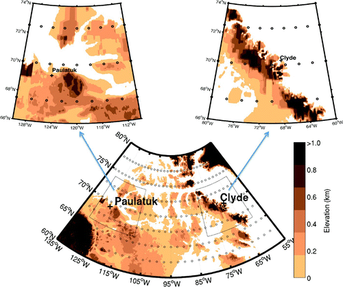
Our interest is in improving and automating wind prediction using more flexible machine learning methods, namely Bayesian neural networks (BNN) and support vector machines for regression (SVR). Three different schemes are designed in this study. Scheme 1 is a statistical downscaling model using daily reforecast data from the National Centers for Environmental Prediction's (NCEP) Global Forecasting System (GFS) as predictors. Scheme 2 uses only previously observed values of the surface wind at the meteorological station as predictors; while Scheme 3 uses the predictors from both Scheme 1 and 2. Observations from two meteorological stations in the Canadian Arctic, Clyde River and Paulatuk (Fig. 1), are used as examples to establish and evaluate our forecast models. Particular attention will be paid to the high-wind event forecasts.

Fig. 1 Topographical map of the Canadian Arctic region, with the Paulatuk and Clyde River stations marked by crosses, and the GFS reforecast model grid points marked by small circles.

Wind observations at the two Canadian stations and the synoptic-scale predictor data from the GFS reforecast data are described in Section 2. Section 3 details the machine learning methods used in this study, with the results given in Section 4, followed by the conclusions in Section 5.

2 Data description

a Surface Wind Measurement

Hourly surface wind speeds during winter (October–March) at two meteorological stations in the Canadian Arctic, Clyde River and Paulatuk, were used in this study. Data records from 1979/80 to 2007/08 for Clyde River and 1987/88 to 2007/08 for Paulatuk were obtained from the Climate Archive web site maintained by MSC.

Clyde River (70.28°N, 68.37°W) is located at the head of Patricia Bay on the east coast of Baffin Island, on flat to gently sloping terrain surrounded by mountains and fjords that have significant impact on the local wind regime. A strong northwesterly surface wind develops when a low-pressure system moves northward through Davis Strait and a ridge of high pressure develops west of Clyde River along eastern Baffin Island, preferentially in winter. Higher terrain to the northwest channels the wind along the coast into Clyde River (Hudson et al., 2001).

Paulatuk (69.22°N, 124.48°W) is located along the western Canadian Arctic coast, at the base of a small but steep escarpment. Strong winter winds (November to April) blow downhill from the Melville Hills in the south, past Paulatuk, and out to sea with a descent of about 200 m within 10 km.

Clyde River and Paulatuk are located in rugged terrain with substantial local effects that influence wind, hence they were chosen for our study instead of flat terrain sites, such as Baker Lake, because the Canadian Global Environmental Multiscale (GEM) model forecasts well at these stations and there are few forecasting challenges. The influence of local topography at Clyde River and Paulatuk are reasonably well understood from a physical point of view but they do present forecasting challenges from day to day. It is particularly difficult to forecast wind at Paulatuk because of a 200 m “cliff” upstream which causes gravity waves to reflect down to the surface under the right conditions (low-level flow at 90° to mid-tropospheric flow when a large-scale mid-troposphere ridge is present). The surface wind can change from light to very strong in less than a minute.

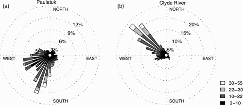
The peak wind speed over a 12 h period, obtained from hourly wind observations, was taken as the predictand in our study. The wind rose diagrams of peak wind speed and direction from the records at Clyde River and Paulatuk are shown in Fig. 2. For Clyde River (Fig. 2b), the dominant wind direction was northwesterly, and most peak winds above 22 knots were also clustered at that direction. For Paulatuk (Fig. 2a), the south and south-southwesterly winds (175°–215°) were very strong statistically. About 30% of the south and south-southwesterly winds are over 22 knots. Compared to Clyde River, Paulatuk has a more complicated wind distribution, with a bimodal distribution manifested in its wind rose due to the strength of the west-southwesterly winds (235°–265°). The likelihood of strong winds is affected by the synoptic weather patterns and local topography.

Fig. 2 Peak wind rose diagrams for (a) Paulatuk and (b) Clyde River. In the legend, “10–22” denotes peak wind speed υ in the range 10 ≤ υ < 22 knots, where 1 knot = 1.852 km h⁻¹ = 0.514 m s⁻¹.

The autocorrelation functions of the peak wind speeds at both sites are given in Fig. 3, showing autocorrelation decreasing, in general, with increasing lag time. The decorrelation time scale or the integral time scale calculated from the autocorrelation function (Hsieh, 2009) for Clyde River and Paulatuk are 2.63 and 3.07 days, separately. These time scales indicate how long the influence of a typical passing weather system lasts and are used to estimate the number of degrees of freedom in the data record, needed later for computing the 95% confidence intervals for the correlations shown in Figs 4 and 5.

Fig. 3 Autocorrelation function of the wind speed as a function of time lag (in days) at Clyde River and Paulatuk.

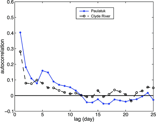
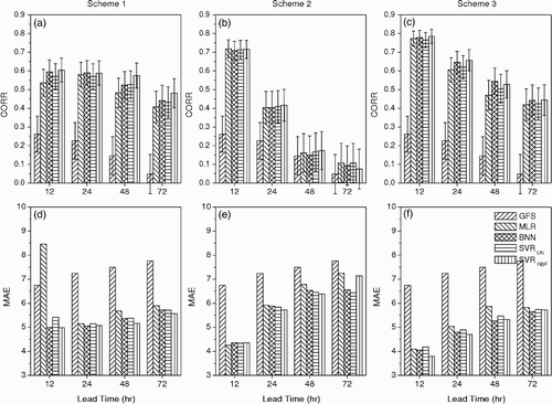
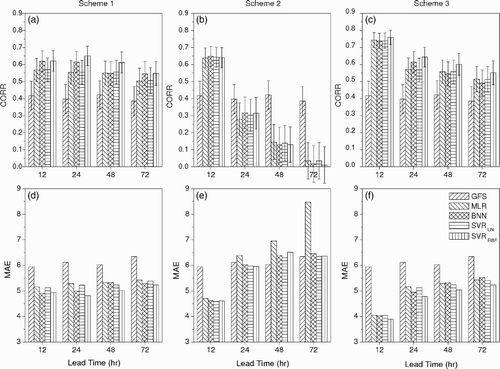
Fig. 4 Comparison of wind forecast performances for Clyde River using CORR and MAE (in knots) produced by different schemes (Schemes 1, 2 and 3) and different methods (raw GFS output, MLR, BNN, SVR_LIN and SVR_RBF) at 12, 24, 48 and 72 h lead times. The 95% confidence intervals for CORR are shown.

Fig. 5 As in Fig. 4 but for Paulatuk.

In this study, we took the immediately preceding wind data, i.e., the peak wind speed, the sine and cosine of the wind direction, the wind speed change (tangential acceleration), and the standard deviation of the wind direction (Weber, 1997) over the previous 12 hours as the five predictors for Scheme 2.

b NCEP GFS Reforecast Data

Synoptic-scale predictors were extracted from the NCEP GFS reforecast dataset (Hamill et al., 2006). GFS reforecast data are retrospective numerical ensemble forecasts from 1979 to the present. An unchanged version of GFS at T62 resolution generated 15-day real-time forecast scenarios (30 time steps of 12 h each), with forecasts run every day from the 00:00 UTC initial conditions. There are 15-member ensemble forecasts that were generated from 15 initial conditions consisting of a reanalysis and seven pairs of bred modes. The datasets have a resolution of 2.5° in both longitude and latitude. The global data were downloaded from the reforecast project file transfer protocol (FTP) server (ESRL, 2008). The field variables include winds, temperature and geopotential heights at the 850, 700, 500, 250 and 150 hPa levels as well as winds and temperature at 1000 hPa, 10 m wind components, 2 m temperature, mean sea level pressure, accumulated precipitation, precipitable water and 700 hPa relative humidity.

The ensemble means (instead of individual ensemble members) of all GFS variables (listed above) on the grid point closest to the station (Clyde River or Paulatuk) are used as predictors. There are a total of 39 predictors, after separating wind direction into its sine and cosine components, and adding the year and day of year as predictors.

3 Methodology

In this study, two non-linear modelling methods, BNN and SVR (introduced below) are applied for wind prediction and tested against multiple linear regression (MLR). Furthermore, three different schemes as mentioned earlier are designed to predict wind speeds at lead times of 12, 24, 48 and 72 h. For these models, the final five years of data were chosen to test the model performances, while the remaining data were used for model training. Prior to training, all input data were scaled to lie within the interval −0.9 to 0.9. Because Schemes 1 and 3 have many predictors, we used stepwise linear regression (Draper and Smith, 1981) to select relevant predictors for all three schemes in this paper to avoid using an excessive number of predictors. The alternative of using the non-liner classification and regression tree (CART) method to select relevant predictors (Faucher et al., 1999) was also tried but did not lead to improved results.

a Bayesian Neural Network

In conventional neural network modelling (Hsieh, 2009), a network is trained using a data set (x, y), where x are the predictors and y the predictand, by adjusting network parameters or weights w to minimize an objective function (also called cost or loss or error function), such as,

where N is the sample size, E _D is an error function measuring how close the network output f(x; w) is to the target y, E _W is the weight penalty term to prevent overfitting, and C is the inverse weight penalty parameter. A small C will strongly suppress the magnitude of w found by the optimization process, thereby yielding a less complex (i.e., less non-linear) model. The best value for C is commonly chosen upon validating the model performance with independent data not used in training the model. With the optimal C, the model should neither overfit nor underfit the data.

An alternative to using validation to find the best value for C is BNN (MacKay, 1992), a neural network design based on a Bayesian probabilistic formulation. The idea of BNN is to treat the network parameters or weights as random variables, obeying an assumed prior distribution. Once observed data are available, the prior distribution is updated to a posterior distribution using Bayes' theorem. BNN automatically determines the optimal value of C without the need of validation data (Hsieh, 2009). In this study, the BNN model from the NETLAB toolbox was used (Nabney, 2002). The number of hidden neurons in the neural network (which determines the number of w parameters) was chosen based on an eight-fold cross-validation (i.e., divide the training data record into eight segments, use only seven for training and reserve one for validation, then rotate the validation data segment until the whole record has been used to validate the model performance). Since the non-linear optimization procedure has multiple local minima, an ensemble of 30 BNN models was built (starting from random initial w), and the ensemble mean was taken as the final wind prediction of the BNN model.

b Support Vector Machine for Regression (SVR)

Support vector machines (SVM) were originally designed for non-linear classification problems (SVC) (Vapnik, 1995), then extended to non-linear regression problems (SVR) (Vapnik et al., 1996). After mapping the input x into a higher dimensional feature space using a non-linear mapping function Φ, the non-linear regression problem between x and y can be converted to a linear regression problem between Φ(x) and y, i.e.,

where ⟨ , ⟩ denotes the inner product, and w and b are the regression coefficients obtained by minimizing the error between f and the observed values of y. To measure this error, instead of the commonly used mean squared error norm, SVR uses the ε-insensitive error norm defined by

i.e., when the difference between f and y is smaller than ϵ, the error is ignored, whereas when the difference between f and y is large, the error approximates the mean absolute error, which is more robust to outliers in the data than the mean squared error. The w and b coefficients are estimated by minimizing the following objective function R using sample data (x _i , y _i ):

where C and ε are prescribed parameters (commonly referred to as hyperparameters).

The main advantage of SVR over neural network models arises from the conversion of a non-linear regression problem to a linear one, Eq. (2), thereby eliminating the need for non-linear optimization, which has local minima in the objective function. However, Φ(x) may be a very high (or even infinite) dimensional vector, hence solving the linear regression problem can be very expensive or impossible to compute without truncating infinite dimensional vectors. In SVR, a kernel trick is used, which is to replace the inner product in the solution algorithm with a kernel function , which does not involve the difficult handling of Φ(x). The minimization of Eq. (4) uses the method of Lagrange multipliers, and the final regression estimate can be expressed in the form (Bishop, 2006):

where the summation is only over a subset of the given data x _i (called the support vectors). Performance of the SVR model depends on the choice of the kernel function and the hyperparameters. In this study, we used the linear kernel, K(x, x _i ) = ⟨x, x _i ⟩, and the Gaussian or radial basis function (RBF) kernel, , with the hyperparameter σ controlling the width of the Gaussian function. SVR with the RBF kernel (SVR_RBF) is a non-linear regression model, while SVR with the linear kernel (SVR_LIN) is a linear regression model — but with the robust ε-insensitive error norm instead of the non-robust mean squared error norm as used in MLR. We used the SVR codes written by Chang and Lin (2001). The hyperparameters were initially estimated according to Cherkassky and Ma (2004) and then optimized by grid searching around the initial values using an eight-fold cross-validation.

4 Results

To verify the forecast performances of different models and schemes, the Pearson correlation coefficient (CORR) and mean absolute error (MAE) were used. While CORR is a good measurement of linear association between the forecasts and observations, it does not take forecast bias into account and is sensitive to outliers. MAE measures the average magnitude of the forecast errors. Compared to the root mean square error (RMSE), MAE is a more unambiguous, hence preferable, measure of the average error (Willmott and Matsuura, 2005).

Figure 4 compares the forecast performance of peak wind speed for Clyde River produced by three different schemes using different methods at lead times of 12, 24, 48 and 72 h. The error bars in the CORR plot give the 95% confidence level of CORR, calculated using the Fisher z transformation (Fisher, 1915) and takes into account the decorrelation time scale. The forecast scores from the 10 m GFS reforecast wind are also presented for reference. For Scheme 1, at all lead times, CORR from the MLR and SVR_LIN models are comparable, while the non-linear models (BNN and SVR_RBF) tend to have slightly (but not significantly) better forecast performance. In addition, all post-processing statistical models clearly perform better than the raw GFS reforecast, which demonstrates the value of statistical downscaling. Up to a 72 h lead, there is no major decline in skill for either the GFS reforecasts or the statistical downscaling models. The same behaviour is found in the MAE scores: the systematic errors of the GFS reforecast are much reduced by the statistical models. Both non-linear statistical models tend to give slightly smaller MAE than the two linear ones.

For Scheme 2, all statistical models provide similar CORR results with a rapid decline in skill as the lead time increases. Only at a 12 h lead time do they perform better than the GFS reforecast — even better than the corresponding forecast from Scheme 1. The very similar CORR values attained by the linear and non-linear statistical models at a 12 h lead indicate that previously observed local wind information only contributes linearly to forecasting future wind speed. For MAE, all statistical models show smaller errors than the GFS reforecast at a 12 h lead time. For longer lead times, the statistical models display comparable MAE relative to the GFS reforecast, except for MLR (which does much worse). Of the three schemes, Scheme 3, by combining the predictors in Schemes 1 and 2, tends to produce the best forecasts at a 12 h lead time. For 24, 48 and 72 h, its forecast scores are quite similar to those of Scheme 1, as the previous observed wind information becomes increasingly irrelevant at longer lead times. At longer lead times, the presence of irrelevant predictors is slightly detrimental to the forecast scores for Scheme 3 relative to Scheme 1, even with the pre-screening of predictors by stepwise regression. Hence, the skill at 12 h comes from the mutual contribution of both the GFS reforecast and previous wind observations; for longer lead times, the skill comes from the GFS reforecast. For Scheme 3, SVR_RBF performs best in both CORR and MAE scores compared with all other methods for all lead times.

Results for Paulatuk are given in Fig. 5. GFS reforecast data performed worse at Paulatuk than at Clyde River, with a smaller CORR (less than 0.3) and larger MAE, and a more rapid drop in forecast performance with increasing lead time. All the post-processing statistical models beat the GFS reforecast. For Scheme 1, among the statistical models, SVR_RBF tends to perform slightly better overall, while MLR tends to attain the poorest scores. For lead times of 12 and 24 h, BNN attains essentially the same scores as SVR_RBF, while for longer lead times of 48 and 72 h, BNN attains essentially the same scores as SVR_LIN, slightly poorer than those attained by SVR_RBF. For Scheme 2, all linear and non-linear statistical models attain very similar CORR, again indicating that only a linear relationship exists between previous local wind information and future wind speed. For Scheme 3, the BNN and SVR_RBF models tend to have marginally better CORR and MAE scores than the two linear models. Compared to Schemes 1 and 2, Scheme 3 gives the best performance at 12 and 24 h lead times. At 48 and 72 h lead times, Scheme 3 has similar to slightly worse forecast scores than Scheme 1, indicating that previously observed wind information is irrelevant.

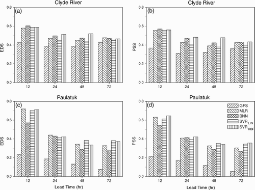
To focus on the forecast performance of different methods for high-wind events (i.e., events with wind speeds greater than 22 knots), we classified the continuous wind forecasts into two classes — high-wind events and non-events. Prior to classification, since the predictions from the statistical models tended to underestimate the amplitude of the wind speed, we rescaled the forecast values, the rescaling calibration was determined by matching the cumulative distribution of the observed wind speed and that of the predicted values using the training data. Only Scheme 3 was used for this analysis. Two forecast scores — the extreme dependency score (EDS) and the Peirce Skill Score (PSS) — were used to verify the resulting binary classification forecasts. EDS (Stephenson et al., 2008) is defined by

where log is the natural logarithm, “hits” is the number of events forecast to occur that did occur, “misses” is the number of events forecast not to occur but did occur, and “total” is the total number of forecasts for occurrences and non-occurrences. EDS ranges from −1 to 1, with a perfect score being 1. EDS is more informative for the assessment of skill in deterministic forecasts of rare events than the traditionally used equitable threat score, which tends to zero for vanishingly rare events. To see how well the forecasts separate the “yes” events from the “no” events, PSS is defined by

where “false alarms” and “correct negatives”, represent the number of times when an event did not occur that was forecast to occur or not to occur, respectively. The value of PSS lies between −1 and 1, with 1 being a perfect forecast. PSS tends to be heavily weighted towards the first term in Eq. (7) for rare events, where the second term becomes very small, as correct negatives tend to vastly outnumber “false alarms”. On the other hand, the EDS is at a disadvantage in that it is defined without taking into account false alarms, i.e., methods can issue more false alarms to enhance their EDS (Primo and Ghelli, 2009).

The EDS and PSS scores of high-wind events forecast using different methods are illustrated in Fig. 6, where all statistical models give better forecast scores than the GFS reforecast, especially at Paulatak. At Clyde River, for a 12 h lead time, non-linear methods do not have an obvious advantage over linear ones, presumably because forecast skill for very short lead times mainly comes from the preceding wind observations which are essentially linearly related to the current wind. For lead times of 24 and 48 h at Clyde River, the non-linear methods, especially SVR_RBF, attained slightly higher scores than the linear methods, though at a 72 h lead time their advantage disappeared. For Paulatuk, the difference in scores between linear and non-linear models became less noticeable than at Clyde River, and BNN generally had the lowest scores. Hence, non-linear regression by BNN and SVR_RBF, which slightly enhanced the continuous forecast scores (CORR and MAE) over the linear models (Figs 4 and 5), failed to do so for the binary forecast scores (EDS and PSS), especially at Paulatuk.

Fig. 6 (a) EDS and (b) PSS scores of high-wind event forecasts using different methods at lead times of 12, 24, 48 and 72 h for Clyde River; and (c) EDS and (d) PSS scores for Paulatuk.

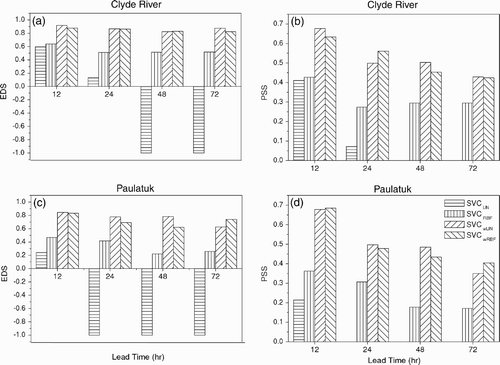
An alternative to using SVR to perform non-linear regression and then classifying the forecasts into high-wind events and non-events is to use the support vector machine directly for classification (SVC), a non-linear classifier, with code supplied by LIBSVM. The EDS and PSS for Clyde River and Paulatuk using SVC with a linear kernel (SVC_LIN) and SVC with an RBF kernel (SVC_RBF) are shown in Fig. 7. The scores are worse than those from our first approach to classifying the SVR forecasts (Fig. 6). In fact, EDS is negative and PSS is zero for SVC_LIN at longer lead times. Since high-wind events occur relatively infrequently compared to non-events, they are difficult for the classifier to forecast correctly. One way to improve the forecasts for rare events is to weight the rare events more heavily than the non-events in the objective function, so the model is trained to emphasize the forecasting of rare events, at the expense of the non-events. With the non-events weighted by unity, the optimal weight for the high-wind events was chosen by cross-validation during the training process of the classifier and found to be around 4 to 6 for the various lead times for both sites. For the optimal weights, the scores over independent test data are shown in Fig. 7, labelled as SVC_wLIN and SVC_wRBF for the two kernels. With weighting, the scores improved substantially from the unweighted model scores, especially with the linear kernel. In fact, with optimal weighting, the linear kernel (SVC_wLIN) attained scores comparable to the RBF kernel (SVC_wRBF). The disadvantage of the weighted models is their tendency to issue more false alarms. The frequency bias, defined by the ratio of the number of events forecast to the number of events observed, is approximately double in the weighted models relative to the unweighted models.

Fig. 7 EDS and PSS of high-wind event forecasts using various support vector classification (SVC) methods at lead times of 12, 24, 48 and 72 h for Clyde River and Paulatuk. SVC_LIN and SVC_RBF use linear and RBF kernels, respectively, while the corresponding “weighted” methods are SVC_wLIN and SVC_wRBF.

5 Summary and conclusions

BNN and SVR with linear and RBF kernels have been developed to predict the surface winds from October to March at two stations (Clyde River and Paulatuk) and compared to the MLR model. Three different forecast schemes were used to identify the contributions to forecast skill from the synoptic-scale GFS reforecast data and from previous local wind observations. In general, for Scheme 1 (with only the GFS reforecast data used as predictors), the non-linear models, BNN and SVR_RBF, have slightly better forecast scores than the linear ones at all lead times for both sites, and SVR_RBF tends to have marginally better scores than BNN. Thus modelling the non-linearity between the GFS reforecast and local surface wind appears to produce forecast scores that are slightly better than those of linear regression models. For Scheme 2 (with only past wind observations used as predictors), the non-linear methods generally have no advantage over the linear methods, and the forecast scores rapidly deteriorate with increasing lead time, indicating that only a linear relation exists between previous local wind observations and the current wind at short lead times. Scheme 3 (combining the predictors from both Schemes 1 and 2) tends to produce the best wind forecasts, especially for shorter lead times.

So far, only predictors from the single closest GFS grid were used. A possible refinement, using predictors from the nine GFS grids closest to the wind station, was tested (not shown), but no clear improvement was found.

Turning from continuous forecasting to binary forecasting of high-wind events and non-events, our first approach was to classify the continuous wind speed predictions into two types — higher than 22 knots (referred to as “high-wind” events) or lower (“non-events”) — and to use EDS and PSS to verify the binary forecasts. For Clyde River, the non-linear methods had slightly better scores than the linear methods at 24 and 48 h lead times. For Paulatuk, all statistical models performed similarly, with BNN performing slightly worse than the others. Hence, non-linear regression by BNN and SVR, which slightly enhanced the continuous forecast scores (CORR and MAE) over the linear models in Figs 4 and 5, generally failed to do so for the binary forecast scores (EDS and PSS) in Fig. 6, especially at Paulatuk.

A second approach performed binary forecasts directly using SVC. The scores were worse than those from our first approach to classifying the SVR forecasts, especially for the linear kernel. After weighting the high-wind events more heavily than the non-events during model training, the scores improved substantially from the unweighted model scores, especially for the linear kernel. With optimal weighting, the linear kernel model (SVC_wLIN) attained similar scores to the RBF kernel model (SVC_wRBF).

In conclusion, we found that wind speed does not have a strong non-linear relation to the GFS reforecast predictors, hence the lack of a major difference between the forecast scores attained by the linear and non-linear downscaling methods. Nevertheless, a slight enhancement in forecast scores by non-linear methods such as SVR appears possible, and binary forecasting of high-wind events can be improved substantially, with the rare events weighted more heavily during model training, though the number of false alarms also increases. Between Clyde River and Paulatuk, Clyde River appeared to benefit from the use of non-linear methods more than Paulatuk. The more complicated bimodal wind speed distribution at Paulatuk (Fig. 2) also seemed to cause BNN, a method vulnerable to local minima during non-linear optimization, to underperform SVR, which does not require non-linear optimization to solve for model weights.

In the future, the methods studied here can be applied to the output from NWP models with much higher horizontal resolution than the GFS model, e.g., the GEM model. Also, the terrain-following vertical coordinates such as the GEM eta-level coordinates would be a better choice than the pressure-level coordinates of the GFS. A major problem with using output from operational NWP models is the frequent upgrades and changes made to operational models, which is one reason for using the GFS reforecast data in this study because the model was held unchanged. Recently, adaptive SVR has been developed (Parrella, 2007) and may be used on output from operational models with frequent upgrades.

Acknowledgements

This work was supported by the Canadian Foundation for Climate and Atmospheric Sciences and the Natural Sciences and Engineering Research Council of Canada. We are grateful for the use of NCEP's GFS reforecast data and helpful discussions with Dr. Alex J. Cannon.

References

- Alexiadis , M. C. , Dokopoulos , P. S. , Sahsamanoglou , H. and Manousaridis , I. M. 1998 . Short-term forecasting of wind speed and related electrical power . Sol. Energy , 63 ( 1 ) : 61 – 68 .
- Barbounis , T. G. and Theocharis , J. B. 2006 . Locally recurrent neural networks for long-term wind speed and power prediction . Neurocomputing , 69 : 466 – 496 .
- Beyer , H. G. , Heinemann , D. , Mellinghoff , H. , Mönnich , K. and Waldl , H.-P. 1999 . Forecast of regional power output of wind turbines . Proceedings of the European Wind Energy Conference EWEC, NICE , (pp. 1062–1065). London, UK: Earthscan Publications Ltd
- Bishop , C. M. 2006 . Pattern Recognition and Machine Learning New York, NY: Springer.
- Chang , C.C. and Lin , C.J. 2001 . LIBSVM: a library for support vector machines [Computer software]. Retrieved 21 March 2008, from http://www.csie.ntu.edu.tw/~cjlin/libsvm
- Cherkassky , V. and Ma , Y. 2004 . Practical selection of SVM parameters and noise estimation for SVM regression . Neural Networks , 17 : 113 – 126 .
- de Rooy , W. C. and Kok , K. 2004 . A combined physical-statistical approach for the downscaling of model wind speeds . Weather Forecast. , 19 : 485 – 495 .
- Draper , N. R. and Smith , H. 1981 . Applied Regression Analysis , 2 New York, NY: Wiley.
- ESRL (Earth System Research Laboratory). 2008. ESRL GFS Reforecast Project [Data file]. Available from http://www.esrl.noaa.gov/psd/people/jeffrey.s.whitaker/refcst
- Faucher , M. , Burrows , W. R. and Pandolfo , L. 1999 . Empirical-statistical reconstruction of surface marine winds along the western coast of Canada . Clim. Res , 11 ( 3 ) : 173 – 190 .
- Fisher , R. A. 1915 . Frequency distribution of the values of the correlation coefficient in samples of an indefinitely large population . Biometrika , 10 : 507 – 521 .
- Gutiérrez , J. M. , Cofiño , A. S. , Cano , R. and Rodríguez , M. A. 2004 . Clustering methods for statistical downscaling in short-range weather forecasts . Mon. Weather Rev. , 132 : 2169 – 2183 .
- Hamill , T. M. , Whitaker , J. S. and Mullen , S. L. 2006 . Reforecasts: an important dataset for improving weather predictions . Bull. Am. Meteorol. Soc. , 97 : 33 – 46 .
- Hanesiak , J. , Stewart , R. , Taylor , P. , Moore , K. , Barber , D. , McBean , G. , Strapp , W. , Wolde , M. , Goodson , R. , Hudson , E. , Hudak , D. , Scott , J. , Liu , G. , Gilligan , J. , Biswas , S. , Desjardins , D. , Dyck , R. , Fargey , S. , Field , R. , Gascon , G. , Gordon , M. , Greene , H. , Hay , C. , Henson , W. , Hochheim , K. , Laplante , A. , Martin , R. , Melzer , M. A. and Zhang , S. 2010 . Storm studies in the Arctic (STAR) . Bull. Am. Meteorol. Soc. , 91 doi: 10.1175/2009BAMS2693.1
- Hsieh , W. W. 2009 . Machine Learning Methods in the Environmental Sciences Cambridge, UK: Cambridge University Press.
- Huang , Q. J. , Hanesiak , J. , Savelyev , S. , Papakyriakou , T. and Taylor , P. 2008 . Visibility during blowing snow events over Arctic sea ice . Weather Forecast. , 23 : 741 – 751 . doi: 10.1175/2008WAF2007015.1
- Hudson , E. , Aihoshi , D. , Gaines , T. , Simard , G. and Mullock , J. 2001 . The Weather of Nunavut and the Arctic: Graphic Area Forecast 36 and 37 (pp. 165–167). Retrieved 12 June 2008, from NavCanada Web site: http://www.navcanada.ca/ContentDefinitionFiles/publications/lak/nunavut/N3637E-W.PDF
- Landberg , L. 2001 . Short-term prediction of local wind conditions . J. Wind Eng. Ind. Aerodyn. , 89 : 235 – 245 .
- MacKay , D. J. C. 1992 . Bayesian interpolation . Neural Comput. , 4 : 415 – 447 .
- Mohandes , M. A. , Halawani , T. O. , Rehman , S. and Hussain , A. A. 2004 . Support vector machines for wind speed prediction . Renew. Energ. , 29 : 939 – 947 .
- Nabney , I. T. 2002 . NETLAB: Algorithms for Pattern Recognition London, UK: Springer.
- Parrella , F. 2007 . Online Support Vector Regression Masters thesis, Department of Information Science, University of Genoa, Italy. Retrieved 27 May 2009, from http://onlinesvr.altervista.org/
- Primo , C. and Ghelli , A. 2009 . The affect of the base rate on the extreme dependency score . Meteorol. Appl. , 16 doi: 10.1002/met.152
- Pryor , S. C. , Schoof , J. T. and Barthelmie , R. J. 2005 . Empirical downscaling of wind speed probability distribution . J. Geophys. Res. , 110: D19109, doi: 10.1029/2005JD005899
- Ricketts , S. and Hudson , E. Climatology and forecasting hazardous weather in Canada's Arctic . Sixth Conference on Polar Meteorology and Oceanography . San Diego, CA: Am. Meteorol. Soc
- Salameh , T. , Drobinski , P. , Vrac , M. and Naveau , P. 2008 . Statistical downscaling of near-surface wind over complex terrain in southern France . Meteorol. Atmos. Phys. , 103 : 253 – 265 .
- Stephenson , D. B. , Casati , B. , Ferro , C. A.T. and Wilson , C. A. 2008 . The extreme dependency score: a non-vanishing measurement for forecasts of rare events . Meteorol. Appl. , 15 : 41 – 50 .
- Vapnik , V. 1995 . The Nature of Statistical Learning Theory New York, NY: Springer-Verlag.
- Vapnik , V. , Golowich , S. E. and Smola , A. 1996 . Support vector method for function approximation, regression estimation, and signal processing . In Advances in Neural Information Processing Systems , (no. 9, pp. 281–287) Cambridge, MA: MIT Press
- Weber , R. O. 1997 . Estimators for the standard deviation of horizontal wind direction . J. Appl. Meteorol. , 36 : 1403 – 1415 .
- Wilby , R. L. and Wigley , T. M.L. 1997 . Downscaling general circulation model output: a review of methods and limitations . Prog. Phys. Geogr. , 21 : 530 – 548 .
- Wilby, R.L.; S.P. Charles, E. Zorita, B. Timbal, P. Whetton and L.O. Mearns. 2004. Guidelines for use of climate scenarios developed from statistical downscaling methods. Retrieved 16 April 2008, from http://proj.badc.rl.ac.uk/dcip/export/1384/ipcc-data.org/trunk/html/guidelines/dgm_no2_v1_09_2004.pdf
- Willmott , J. and Matsuura , K. 2005 . Advantages of the mean absolute error (MAE) over the root mean square error (RMSE) in assessing average model performance . Clim. Res. , 30 : 78 – 82 .