Long-Term Ozone Changes Over the Northern Hemisphere Mid-Latitudes for the 1979–2012 Period

Abstract

The solar backscattered ultraviolet (SBUV/SBUV-2) merged ozone datasets, version 8.6, including column ozone and ozone profiles for the 1979–2012 period are examined for the 35°N–60°N zonal belt in the northern hemisphere mid-latitudes and four sub-regions: central Europe, continental Europe, North America, and East Asia. The residual long-term patterns for total ozone and ozone profiles are extracted by smoothing the time series of differences between the original and the modelled ozone time series. Modelled ozone is obtained using the standard trend model accounting for ozone variability due to changes in stratospheric halogens and various dynamical factors commonly used in previous ozone trend analyses. Since about 2005 spring and summer total ozone in the troposphere and lower stratosphere has decreased in some regions (central and continental Europe, North America, and the 35°N–60°N zonal belt) compared with modelled ozone. The negative departure from modelled ozone in 2010 is approximately 2–3% of the overall 1979–2012 monthly mean level. It seems that this decrease is a result of yet unknown dynamical processes rather than to chemical destruction because the differences have a longitudinal structure, and total ozone in the upper stratosphere still follows changes in stratospheric halogen loading.

Résumé

[Traduit par la rédaction] Nous examinons les ensembles de données d'ozone fusionnés fournis par les radiomètres ultraviolet de rétrodiffusion solaire (SBUV/SBUV–2), version 8.6, qui incluent la colonne d'ozone et les profils d'ozone pour la période 1979–2012, pour la ceinture zonale 35°N–60°N dans les latitudes moyennes de l'hémisphère Nord et quatre sous-régions : l'Europe centrale, l'Europe continentale, l'Amérique du Nord et l'Asie orientale. Les configurations résiduelles à long terme pour l'ozone total et les profils d'ozone sont extraites en lissant la série temporelle des différences entre les séries temporelles d'ozone originale et modélisée. L'ozone modélisé est obtenu en utilisant le modèle de tendance standard qui tient compte de la variabilité de l'ozone due aux changements dans les halogènes stratosphériques et à différents facteurs couramment utilisés dans les analyses de tendance d'ozone précédentes. Depuis 2005 environ, l'ozone total au printemps et en été dans la troposphère et la basse stratosphère a diminué dans certaines régions (Europe centrale et continentale, Amérique du Nord et ceinture zonale 35°N–60°N) comparativement à l'ozone modélisé. L’écart négatif par rapport à l'ozone modélisé en 2010 est approximativement de 2 à 3% du niveau mensuel moyen d'ensemble pour 1979–2012. Il semble que cette diminution soit attribuable à des processus dynamiques encore inconnus plutôt qu’à une destruction chimique parce que les différences ont une structure longitudinale et l'ozone total dans la haute stratosphère suit encore les changements dans la charge d'halogènes stratosphériques.

Keywords:

• ozone recovery
• Montreal Protocol 1987
• trend
• dynamical/chemical drivers
• northern hemisphere
• mid-latitudes

1 Introduction

The stratospheric ozone depletion over extratropical regions that has been observed since the 1970s alarmed the scientific community because thinning of the ozone layer would result in more intense ultraviolet-B (UV-B) radiation reaching the Earth's surface. Excessive UV-B radiation is linked to adverse effects on various ecosystems and human health. Depletion of stratospheric ozone began to level off in the mid-1990s after a strong decrease in ozone during the preceding two decades. Several authors have indicated that such a change in the ozone trend pattern could be linked to the success of the Montreal Protocol of 1987 and its later amendments that set limits on the production of ozone-depleting substances (ODSs; e.g., Morgerstern et al., 2008; Velders, Andersen, Daniel, Fahey, & McFarland, 2007).

The World Meteorological Organization (WMO, 2007) defined the following stages of ozone recovery: (i) slowing of the downward trend in the ozone time series, (ii) onset of the upward trend in the ozone time series, and (iii) return to pre-1980 ozone levels in the stratosphere. Recent WMO reports on the state of the ozone layer (WMO, 2007, 2011) corroborated that the increase in atmospheric contamination by ODSs was mostly responsible for ozone depletion in the extratropics in the 1980s and in the early 1990s. Afterwards, ozone in the mid-latitudes showed the first sign of recovery with the appearance of a slight increase from the mid-1990s minimum. Thus, the beginning of the second recovery stage could be announced (e.g., Angell & Free, 2009; Krzyścin, 2012; Krzyścin, Jarosławski, & Rajewska-Więch, 2005; Mäder et al., 2010; Weatherhead & Andersen, 2006; Yang et al., 2006).

Interannual fluctuations in atmospheric ozone come from a superposition of components due to changes in atmospheric chemistry (mostly related to changes in ODSs) and those induced by the dynamical processes affecting the ozone layer. In order to study causes of long-term variability of atmospheric ozone, it is necessary to separate dynamically driven variations from chemical ones. Multiple linear regression analyses were carried out to identify sources of long-term ozone variability (e.g., Harris et al., 2008; Mäder et al., 2007; Reinsel et al., 2005).

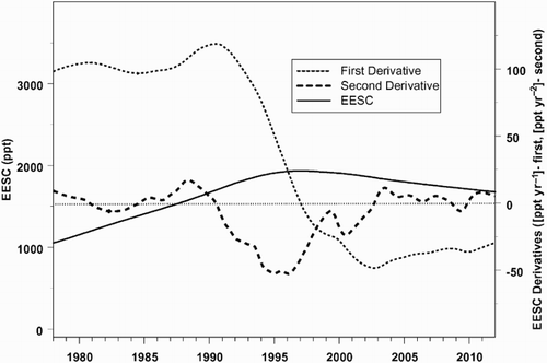
The portion of the ozone trend resulting from changes in ODSs was calculated as proportional to the equivalent effective stratospheric chlorine (EESC) loading. The EESC peaked at different times in mid- and high latitude regions (Daniel et al., 2007). The EESC concentration is much higher in polar regions because a stratospheric air parcel has a longer mean age. This has a higher potential for ozone destruction (Newman, Daniel, Waugh, & Nash, 2007). The date when the second derivative of the EESC reaches a minimum is defined as the onset of the ozone increase (Yang et al., 2006). This happened in the mid-latitudes around 1996 (Fig. 1). Based on the EESC pattern, it was estimated that a significant amount of ozone would be recovered in the mid-latitudes by the end of 2012.

Fig. 1 Equivalent effective stratospheric chlorine (EESC) calculated for the mid-latitude stratosphere (solid line). Dotted and dashed lines represent the first and second derivatives of EESC, respectively.

Here we examine the differences between the observed pattern of mid-latitude ozone and the modelled pattern that includes an anthropogenic trend component due to EESC changes. The standard multivariate linear trend model with commonly used proxies is used to identify sources of ozone variability. Our intent is to examine the long-term variability of a residual part of the trend model (i.e., the ozone time series that remains after subtracting the modelled ozone from the observed ozone). This allows us to determine whether the long-term pattern of mid-latitude ozone follows the recent decrease in atmospheric contamination by halogens resulting from the Montreal Protocol of 1987 on substances that delete the ozone layer and its subsequent amendments.

2 Data

The solar backscattered ultraviolet (SBUV) merged total and profile ozone datasets (MOD), version 8.6 (available at http://acd-ext.gsfc.nasa.gov/Data_services/merged/), for the 1979–2012 period were analyzed to estimate causes of long-term total ozone variability in the northern hemisphere mid-latitudes. The MOD contains homogenized records from the Nimbus 7 SBUV instrument and a series of SBUV/2 instruments onboard various National Oceanic and Atmospheric Administration (NOAA) satellites. The MOD appears suitable for trend analyses (Chehade, Burrows, & Weber, 2013; DeLand, Taylor, Huang, & Fisher, 2012; Kramarova et al., 2013). The monthly mean values of the column amount of ozone, as well as the total ozone in the troposphere and lower stratosphere (1013–25.45 hPa) and in the upper stratosphere (4.034–1.013 hPa), were examined over the 35°N–60°N zonal belt. Using MOD overpass data (available at ftp://toms.gsfc.nasa.gov/pub/sbuv/MERGED/), total and selected ozone profile data were obtained for the following northern hemisphere regions: central Europe (40°N–55°N, 5°E–25°E), continental Europe (35°N–60°N, 15°W–45°E), East Asia (35°N–60°N, 85°E–145°E), and continental North America (35°N–60°N, 130°W–70°W). The statistical analyses were carried out on a seasonal basis: winter (December, January, and February), spring (March, April, and May), summer (June, July, and August), and autumn (September, October, and November).

Monthly mean ozone data were converted to so-called fractional deviations, δO₃(t), defined as follows:(1)

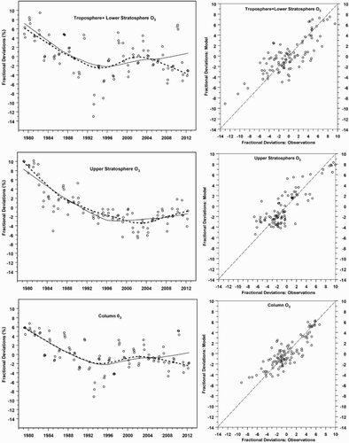
where t is the running month equal to (year –1979) × 12 + M, t = 1 in January 1979, O₃(t) denotes the monthly mean of total ozone or ozone amount in the troposphere and lower stratosphere (Tr-LSt) or in the upper stratosphere (USt) in month t, O₃(M) is the long-term (1979–2012) monthly mean for calendar month M corresponding to t. Figure 2 shows the fractional ozone deviations for the spring subset of the MOD data.

Fig. 2 (left column) Monthly fractional deviations (points) of the 35°–60°N mean ozone for spring (MAM) during the 1979–2012 period. (top panel) ozone content in the troposphere and lower stratosphere; (middle panel) ozone content in the upper stratosphere; (bottom panel) total ozone. The solid and dotted curves show the smoothed (by locally weighted regression – LOWES) pattern of the modelled and original data, respectively. (right column) modelled versus observed monthly fractional deviations of the profile and total ozone corresponding to the panels in the left column.

Following previous statistical studies on ozone variability (e.g., Chehade et al., 2013; Frossard et al., 2013; Krzyścin, Rajewska-Więch, & Jarosławski, 2013; Mäder et al., 2010) the following set of ozone proxies were selected (i.e., the variables that could explain ozone variability in a multivariate regression model): (i) EESC to parameterize the influence of ODSs on atmospheric ozone; (ii) the zonal component of the wind at 30 and 50 hPa averaged over the tropics for the Quasi-Biennial Oscillation (QBO) attribution; (iii) the Arctic Oscillation (AO) index; (iv) Penticton/Ottawa 2800 MHz solar flux to search for 11-year solar cycle effects; (v) the El Niño/Southern Oscillation (ENSO) index, sea surface temperature (SST) anomalies in the Niño-3.4 region used for global atmospheric disturbances induced by quasi-periodical sea surface temperature fluctuations in the equatorial Pacific; (vi) the cumulative Eliassen-Palm (EP) flux at 100 hPa averaged over the 45°N–75°N region for a description of ozone changes induced by the variability of the Brewer-Dobson circulation; and (vii) stratospheric aerosol optical depth at 550 nm for attribution of the ozone variability resulting from volcanic eruptions. Details and web addresses of the ozone proxies can be found in Krzyścin et al. (2013).

3 Model

A standard multivariate regression model was used to explain the variability of atmospheric ozone. The time series of monthly fractional deviations is supposed to be a linear superposition of components related to the ozone response to specific chemical and dynamical processes:(2)

where α_oEESC(t) represents the anthropogenic trend component of the ozone time series related to the stratospheric halogen concentration changes described by the EESC time series (see Fig. 1), and α_iX_i(t) represents the time series due to specific dynamical or chemical forcing on the ozone layer. The model includes components related to changes in the 11-year solar activity, QBO, ENSO, AO, Brewer-Dobson circulation, and the stratospheric aerosol optical depth (Section 2). Regression constants α_( … ) are calculated by a standard least-squares fit. Noise(t) represents an unresolved part of the time series that is assumed to be a sum of the long-term and short-term components, Noise_L(t) and Noise_S(t), respectively, (3)

Noise_L(t) is extracted from the Noise(t) time series using a locally weighted scatterplot LOWESS smoother (Cleveland, 1979). The level of smoothing is arbitrarily chosen to retain components with time scales longer than about a decade; Noise_S(t) is the remaining part of the time series containing the short-term oscillations.

The bootstrap set of Noise_L(t) terms was built to estimate the uncertainty range of this component. A hypothetical nth representative of the Noise_L(t) term, Noise_L(n)(t), n = (1, … .1000), was created by adding random values from the Noise_S(t) term to the Noise_L(t) time series then applying the LOWES smoother to this new time series. Finally, the 95% confidence interval for moment t was calculated taking the 2.5 and 97.5 percentile from the ordered (from lowest to highest) n = 1000 values of the Noise_L(n)(t) time series.

Equation (2) was run separately for the winter (DJF), spring (MAM), summer (JJA), and autumn (SON) subsets of the column amount and profile (Tr-LSt and USt) ozone data. Such a multivariate regression model has commonly been used to find sources of atmospheric ozone variability. Examination of the ozone response to the selected proxy has been the main subject of many previous statistical analyses (e.g., Chehade et al., 2013; Harris et al., 2008; Reinsel et al., 2005) and is not discussed here. Here we focus on the variability of the Noise_L(t) term that provides a performance test for the multilinear regression model with the trend term being proportional to the EESC time series. Thus, it is possible to estimate the extent to which long-term ozone variability is forced by changes in stratospheric halogen. In this way, the effectiveness of the Montreal Protocol on substances that deplete the ozone layer, and its subsequent amendments, can also be determined.

4 Results

The modelled and observed total and profile northern hemisphere mid-latitude ozone for the 1979–2012 spring seasons are shown in Fig. 2. The modelled fractional deviations reproduce the observed ones (right column of Fig. 2). The correlation coefficients between the modelled and observed data are 0.8, 0.86, and 0.85 for Tr-LSt, USt, and the entire atmosphere, respectively. This means that the model can explain a significant portion of the observed variability in ozone data. There is good agreement between the smoothed patterns of the modelled and observed data (see curves in the left panels of Fig. 2). The modelled patterns show there has been a continuous increase in total and profile ozone data since the mid-1990s (i.e., the period of decreasing concentration of ODSs in the stratosphere). However, total and Tr-LSt ozone start to diverge from the modelled ones in about 2005. This is more pronounced in the Tr-LSt data. The modelled and observed ozone show the second stage of the ozone recovery in the upper stratosphere during the 1996–2012 period. The observations show that there has been no further ozone depletion since the mid-1990s suggesting that the first stage of the ozone recovery in the whole column and in Tr-LSt has occurred.

A question arises as to whether such a negative departure in the ozone observations from the modelled values in these layers is statistically significant or is due to a statistical anomaly due to the appearance of many low ozone values at the end of the time series. Analyses of the uncertainty range of the long-term component of the noise (Eq. (3)) provide the answer.

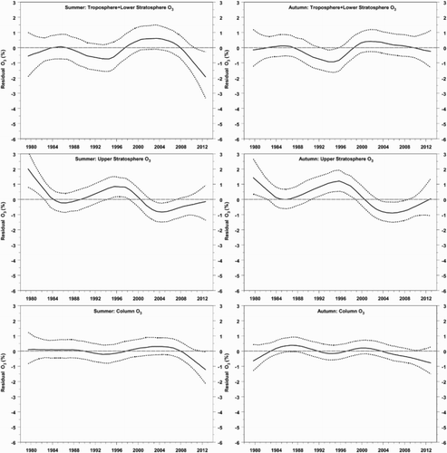
Figures 3 to 4 show the residual trend pattern in the northern hemisphere mid-latitudes (35°N–60°N) total and profile ozone for all seasons of the year for the 1979–2012 period. It can be seen that the decreasing tendency is statistically significant in spring and summer in the Tr-LSt region and marginally statistically significant in the column ozone in these periods.

Fig. 3 The solid curves show the smoothed differences between the observed and modelled fractional deviations of total ozone in (top panels) the troposphere and lower stratosphere, (middle panels) the upper stratosphere, and (bottom panels) the entire atmosphere during the 1979–2012 period for the 35°N–60°N zonal belt in winter (left column) and spring (right column). The dotted curves show the 95% confidence interval for these differences.

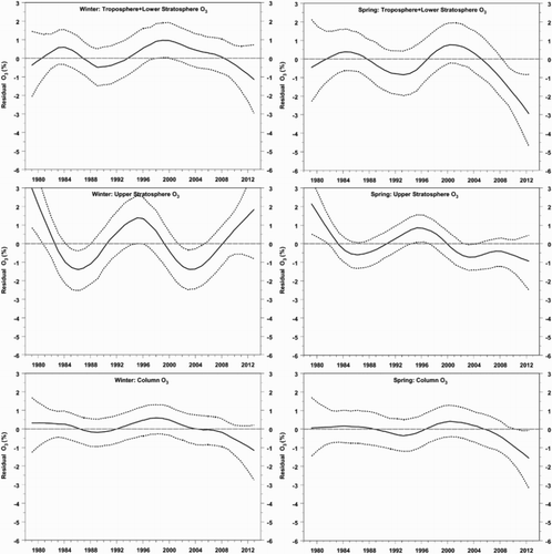
Fig. 4 As in Fig. 3 but for the smoothed differences in summer and autumn.

Table 1 presents values of the residual trend pattern in 2010 for all seasons considered and the northern hemisphere mid-latitude sub-regions. The uncertainty range for the trend pattern increases at the edges of the curve; thus, the year 2010 was selected for calculations (see time series shown in Fig. 3). The statistically significant negative values of the residual ozone in the Tr-LSt layer are found in spring and summer in central Europe, continental Europe, and in the entire 35°N–60°N zone, but only in summer for the North American region. Similar results but smaller negative values are found for the column ozone residuals with the exception of the summer data for the entire 35°N–60°N region.

Table 1. Seasonal differences (percentage of the 1979–2012 mean values) in 2010 between the observed and modelled fractional deviations of the amount of ozone in the troposphere and lower stratosphere (Tr-LSt), the upper stratosphere (USt), and in the entire atmospheric column (Column) for various northern hemisphere mid-latitude regions and the 35°N–60°N zone. The 95% confidence intervals for the differences are in parentheses and statistically significant results are in bold.

Season	Layer	Central Europe	Continental Europe	North America	East Asia	Zone 35°–60°N
Winter	Tr-LSt	−1.1 (−3.6, 1.2)	−0.6 (−2.5, 1.2)	1.3 (−0.6, 3.2)	−0.1 (−1.8, 1.2)	−0.5 (−1.7, 0.6)
	USt	0.4 (−1.8, 2.1)	0.4 (−1.5, 2.1)	1.4 (−0.1, 2.8)	1.4 (−0.5, 3.2)	1.0 (−0.5, 2.3)
	Column	−1.4 (−3.3, 0.5)	−1.3 (−2.8, 0.3)	0.7 (−0.8, 2.0)	−0.7 (−1.9, 0.3)	−0.8 (−1.9, 0.2)
Spring	Tr-LSt	−2.8 (−4.5,−0.8)	−2.3 (−3.8,−0.7)	−1.5 (−3.4, 0.4)	−1.4 (−3.0, 0.4)	−2.0 (−3.2,−0.5)
	USt	0.5 (−0.7, 1.4)	0.4 (−0.7, 1.3)	−0.2 (−1.2, 1.0)	−0.8 (−2.0, 0.2)	−0.6 (−1.5, 0.2)
	Column	−1.6 (−3.1,−0.3)	−1.2 (−2.5,−0.1)	−0.7 (−2.0, 0.5)	−1.0 (−2.2, 0.2)	−1.0 (−2.0,−0.1)
Summer	Tr-LSt	−2.2 (−3.4,−1.1)	−2.0 (−2.8,−1.0)	−1.5 (−2.6,−0.6)	−1.1 (−2.4, 0.7)	−1.2 (−1.9,−0.1)
	USt	−0.2 (−1.0, 0.6)	−0.1 (−0.9, 0.6)	−0.1 (−1.0, 0.7)	0.0 (−0.8, 0.7)	−0.3 (−1.0, 0.4)
	Column	−1.3 (−1.9,−0.6)	−1.2 (−1.6,−0.6)	−0.8 (−1.3,−0.3)	−0.6 (−1.3, 0.4)	−0.7 (−1.2, 0.1)
Autumn	Tr-LSt	−0.9 (−2.0, 0.6)	−0.6 (−1.4, 0.6)	−0.2 (−1.1, 0.8)	−0.4 (−1.6, 0.7)	−0.1 (−0.8, 0.9)
	USt	−0.5 (−1.2, 0.3)	−0.6 (−1.2, 0.3)	−0.3 (−0.9, 0.6)	−0.3 (−1.1, 0.5)	−0.3 (−1.0, 0.5)
	Column	−0.8 (−1.5, 0.2)	−0.7 (−1.2, 0.3)	−0.4 (−1.0, 0.2)	−0.5 (−1.2, 0.2)	−0.6 (−1.1, 0.1)

5 Discussion and conclusions

The 1987 Montreal Protocol on substances that deplete the ozone layer, and its subsequent amendments, led to a decrease in halogen concentration in the stratosphere starting in the mid-1990s. However, some substances affecting atmospheric ozone (e.g., nitrous oxide (N₂O)) were not monitored. Present estimates show that N₂O will be the most important ozone-depleting chemical throughout the twenty-first century (Kanter et al., 2013; Ravishankara, Daniel, & Portmann, 2009).

Long-term changes in atmospheric ozone were determined using a multiple regression model with the trend term parameterized by EESC time series showing an increasing tendency up to the mid-1990s followed by a slight decreasing tendency afterwards. Such tendency overturning could be linked to halogen production limits forced by regulations under the 1987 Montreal Protocol and its subsequent amendments. The increase in ozone during the EESC decreasing phase is rather automatically forced by the ozone behaviour before the EESC overturning when the strong increase in EESC occurred along with the strong decrease in ozone. This resulted in a high negative value for the regression coefficient pertaining to the EESC proxy in the multivariate regression model and induced a positive ozone trend in the decreasing EESC phase.

We analyzed the residual trend pattern extracted from the remaining part of the ozone series after subtracting the modelled time series from the observed time series. In this way the performance of the standard regression model with the trend term proportional to changes in halogen could be verified. Moreover, a combined forcing of other factors with chemical (e.g., increase in N₂O) and/or dynamical (not yet parameterized in the regression models) origins could be estimated.

The statistical analyses of the residual trend pattern showed that the upper stratosphere trend in ozone during the 1979–2012 period has a mostly chemical origin related to the changes in halogen. In spring and summer, tropospheric and lower stratospheric ozone start to depart from the modelled values after about 2005 in some mid-latitude regions (central Europe, continental Europe, and North America) and in the 35°N–60°N mid-latitude zonal belt. The negative departure from the modelled Tr-LSt ozone in 2010 was found to be about 2–3% relative to the 1979–2012 ozone mean. Comparing values modelled by multivariate regression, the column amount of ozone also has lower values at the end of the time series but the decrease is slightly less than that found in the combined troposphere and lower stratosphere layer.

The 1987 Montreal Protocol and its subsequent amendments have been successful because the long-term ozone pattern generally agrees with the changes in EESC throughout almost the entire period examined. The negative deviation from the modelled pattern is found only in the lower layers of the atmosphere, near the end of the time series. There are regional differences in the statistical significance of this decrease, the most evident being in central Europe. It seems that this decrease is due to unknown dynamical processes rather than to chemical destruction processes, for example, to increasing stratospheric N₂O, because the differences have longitudinal structure, and the ozone content in the upper stratosphere still follows the EESC pattern. It is difficult to envisage whether the recovery date for northern hemisphere mid-latitude ozone is later that expected from scenarios assuming decreasing contamination of the stratosphere by halogens in the twenty-first century. Monitoring of atmospheric ozone is still an important scientific issue because the origins of the latest fluctuations in northern hemisphere mid-latitude ozone are unclear.

Acknowledgements

This work was partially supported by National Science Centre grant number UMO-2011/01/B/ST10/06892. The research was also supported within statutory activities No 3841/E-41/S//2014.

References

- Angell, J. K., & Free, M. (2009). Ground-based observations of the slowdown in ozone decline and onset of ozone increase. Journal of Geophysical Research, 114, D07303. doi: 10.1029/2008JD010860
- Chehade, W., Burrows, J. P., & Weber, M. (2013). Total ozone trends and variability during 1979–2012 from merged datasets of various satellites. Atmospheric Chemistry and Physics Discussions, 13, 30407–30452. doi: 10.5194/acpd-13-30407-2013
- Cleveland, W. S. (1979). Robust locally weighted regression and smoothing scatterplots. Journal of the American Statistical Association, 74, 829–836. doi: 10.1080/01621459.1979.10481038
- Daniel, J. S., Velders, G. J., Douglass, A. R., Forster, P. M. D., Hauglustaine, D. A., Isaksen, I. S., … Wallington, T. J. (2007). Halocarbon scenarios, ozone depletion potentials, and global warming potentials. In Chapter 8: Scientific assessment of ozone depletion: 2006 (pp. 8.1–8.40). Global Ozone: Research. and Monitoring Project – Report No. 50, Geneva: World Meteorological Organization.
- DeLand, M. T., Taylor, S. L., Huang, L. K., & Fisher, B. L. (2012). Calibration of the SBUV version 8.6 ozone data product. Atmospheric Measurement Techniques, 5, 2951–2967. doi: 10.5194/amt-5-2951-2012
- Frossard, L., Rieder, H. E., Ribatet, M., Staehelin, J., Maeder, J. A., Di Rocco, S., … Peter, T. (2013). On the relationship between total ozone and atmospheric dynamics and chemistry at mid-latitudes – Part 1: Statistical models and spatial fingerprints of atmospheric dynamics and chemistry. Atmospheric Chemistry and Physics, 13, 147–164. doi: 10.5194/acp-13-147-2013
- Harris, N. R. P., Kyrö, E., Staehelin, J., Brunner, D., Andersen, S.-B., Godin-Beekmann, S., … Zerefos, C. (2008). Ozone trends at northern mid- and high latitudes – a European perspective. Annales Geophysicae, 26, 1207–1220. doi: 10.5194/angeo-26-1207-2008
- Kanter, D., Mauzerall, D. L., Ravishankara, A. R., Daniel, J. S., Portmann, R. W., Grabiel, P. M., … Galloway, J. N. (2013). A post-Kyoto partner: Considering the stratospheric ozone regime as a tool to manage nitrous oxide. Proceedings of the National Academy of Sciences of the United States of America, 110 (12), 4451–4457. doi:10.1073/pnas.1222231110
- Kramarova, N. A., Frith, S. M., Bhartia, P. K., McPeters, R. D., Taylor, S. L., Fisher, B. L., … DeLand, M. T. (2013). Validation of ozone monthly zonal mean profiles obtained from the version 8.6 solar backscatter ultraviolet algorithm. Atmospheric Chemistry and Physics, 13, 6887–6905. doi: 10.5194/acp-13-6887-2013
- Krzyścin, J. W. (2012). Onset of the total ozone increase based on statistical analyses of global ground-based data for the period 1964–2008. International Journal of Climatology, 32, 240–246. doi:10.1002/joc.2264
- Krzyścin, J. W., Jarosławski, J., & Rajewska-Więch, B. (2005). Beginning of the ozone recovery over Europe? – Analysis of the total ozone data from the ground-based observations, 1964–2004. Annales Geophysicae, 23, 1–11. doi: 10.5194/angeo-23-1685-2005
- Krzyścin, J. W., Rajewska-Więch, B., & Jarosławski, J. (2013). The long-term variability of atmospheric ozone from the 50-yr observations carried out at Belsk (51.84°N, 20.78°E), Poland. Tellus B, 65, 21779. doi:10.3402/tellusb.v65i0.21779
- Mäder, J. A., Staehelin, J., Brunner, D., Stahel, W. A., Wohltmann, I., & Peter, T. (2007). Statistical modeling of total ozone: Selection of appropriate explanatory variables. Journal of Geophysical Research, 112, D11108. doi:10.1029/2006JD007694
- Mäder, J. A., Staehelin, J., Peter, T., Brunner, D., Rieder, H. E., & Stahel, W. A. (2010). Evidence for the effectiveness of the Montreal Protocol to protect the ozone layer. Atmospheric Chemistry and Physics, 10, 12161–12171. doi: 10.5194/acp-10-12161-2010
- Morgenstern, O., Braesicke, P., Hurwitz, M. M., O'Connor, F. M., Bushell, A. C., Johnson, C. E., … Pyle, J. A. (2008). The world avoided by the Montreal Protocol. Geophysical Research Letters, 35, L16811. doi:10.1029/2008gl034590
- Newman, P. A., Daniel, J. S., Waugh, D. W., & Nash, E. R. (2007). A new formulation of equivalent effective stratospheric chlorine (EESC). Atmospheric Chemistry and Physics, 7, 4537–4552. doi: 10.5194/acp-7-4537-2007
- Ravishankara, A. R., Daniel, J. S., & Portmann, R. W. (2009). Nitrous oxide (N2O): The dominant ozone-depleting substance emitted in the 21st century. Science, 326(5949), 123–125. doi:10.1126/science.1176985
- Reinsel, G. C., Miller, A. J., Weatherhead, E. C., Flynn, L. E., Nagatani, R. M., Tiao, G. C., … Wuebbles, D. J. (2005). Trend analysis of total ozone data for turnaround and dynamical contributions. Journal of Geophysical Research, 110, D16306. doi:10.1029/2004JD004662
- Velders, G. J., Andersen, S. O., Daniel, J. S., Fahey, D. W., & McFarland, M. (2007). The importance of the Montreal Protocol in protecting climate. Proceedings of the National Academy of Sciences of the United States of America, 104, 4814–4819. doi:10.1073/pnas.0610328104
- Weatherhead, E. C., & Andersen, S. B. (2006). The search for signs of recovery of the ozone layer. Nature, 441, 39–45. doi:10.1038/nature04746
- World Meteorological Organization. (2007). Scientific assessment of ozone depletion: 2006, Report 50, Global Ozone Research and Monitoring Project, Geneva.
- World Meteorological Organization. (2011). Scientific assessment of ozone depletion: 2010, Report 52, Global Ozone Research and Monitoring Project, Geneva.
- Yang, E.-S., Cunnold, D. M., Salawitch, R. J., McCormick, M. P., Russell III, J., Zawodny, J. M., … Newchurch, M. J. (2006). Attribution of recovery in lower-stratospheric ozone. Journal of Geophysical Research, 111, D17309. doi:10.1029/2005JD006371