Predicting Snow Depth in a Forest–Tundra Landscape using a Conceptual Model Allowing for Snow Redistribution and Constrained by Observations from a Digital Camera

abstract

Estimation of snow depth in the forest–tundra landscape remains a challenge because of a lack of reliable and frequent observations on precipitation and snow depth. Snow models forced by gridded meteorological datasets are often the only option available for assessing snow depth at the local scale. Unfortunately, these models generally do not take into account the snow redistribution process between open and forested areas which frequently occurs in the forest–tundra landscape. A simple modification to an existing snow accumulation and melt model is proposed in order to allow for snow redistribution. Along with a technique for taking advantage of snow depth observations obtained from a digital camera, the model is shown to provide accurate predictions of snow depth at the local scale when forced with precipitation data from Environment Canada's Canadian Precipitation Analysis. Results from this study suggest that instrumenting automated weather stations with a digital camera, together with small modifications to an existing model used operationally for snow depth prediction, could result in significant improvements to snow depth prediction and analysis in this environment. Further testing at sites where snow water equivalent of the snowpack is available should, however, be performed to fully validate the method.

RÉSUMÉ

[Traduit par la rédaction] L'estimation de l’épaisseur de la neige dans les régions de toundra forestière demeure difficile à cause du manque d'observations fiables et fréquentes des précipitations et de l’épaisseur de la neige. Les modèles de neige forcés par des ensembles de données météorologiques à des points de grilles constituent souvent le seul moyen d’évaluer l’épaisseur de la neige à l’échelle locale. Malheureusement, ces modèles ne tiennent habituellement pas compte du processus de redistribution de la neige entre terrains ouverts et terrains boisés qui se produit souvent dans les régions de toundra forestière. Nous proposons une modification simple à un modèle existant d'accumulation et de fonte de neige afin de permettre la redistribution de la neige. Utilisé de pair avec d'une technique permettant de prendre avantage des observations d’épaisseur de neige fournie par un appareil photo numérique, le modèle s'avère capable produire des prévisions d’épaisseur de neige précises à l’échelle locale lorsqu'il est forcé avec les données de l'Analyse canadienne des précipitations d'Environnement Canada. Les résultats de cette étude suggèrent qu'en équipant les stations météorologiques automatisées d'un appareil photo numérique et en apportant de petites modifications au modèle utilisé opérationnellement pour la prévision de l’épaisseur de neige, la prévision et l'analyse de l’épaisseur de la neige dans cet environnement pourraient s'en trouver grandement améliorées. Il faudrait, toutefois, faire d'autres tests à des sites où l’équivalent en eau de l'accumulation de neige est disponible pour valider pleinement la méthode.

Keywords:

• snow depth
• subarctic forest-tundra
• monitoring
• modelling
• camera

1 Introduction

Information on snow depth is useful for a number of environmental prediction applications, including reservoir inflow forecasting (Singh, Mishra, Thakur, Kulkarni, & Singh, 2009), flood forecasting (Todhunter, 2001), weather forecasting (Dutra et al., 2010), and forest fire prediction (Westerling, Hidalgo, Cayan, & Swetnam, 2006). The amount of snow on the ground during winter also has a strong impact on carbon fluxes and ground temperature (Stieglitz, Dery, Romanovsky, & Osterkamp, 2003) and, hence, on the ecosystem at large. In open areas, snow depth can be obtained from passive microwave remote sensing retrievals, but this is much more challenging in forested areas (Derksen, Walker, & Goodison, 2003). Routine ground observations of snow depth are often available from non-automated weather stations, which are generally located in relatively accessible areas, generally at lower elevations than the surroundings (Brasnett, 1999), and biased to coastal locations in the Canadian North (Brown, Derksen, & Wang, 2007). In more remote locations, some automated stations are equipped with ground pointing sonars which can estimate snow depth at a single point (Varhola et al., 2010). However, in a complex landscape snow depth is, to a large extent, controlled by the local topography and vegetation and, thus, can change significantly over short distances (Vajda, Venülainen, Hanninen, & Sutinen, 2006). Variations in snow depth across the landscape can be captured with a digital camera; although such observations are not generally available from operational weather stations, the technique has been used successfully by researchers to monitor changes in snow extent and snow depth remotely in complex environments (Hinkler, Pedersen, Rasch, & Hansen, 2002; Parajka, Haas, Kimbauer, Jansa, & Bloschl, 2012). The simplest application of a digital camera for monitoring snow depth consists of pointing the camera at a number of snow rulers installed throughout the landscape and estimating snow depth at each site from the digital images.

In remote locations not easily serviceable during winter, obtaining frequent digital images of the landscape throughout the winter can be quite challenging. In particular, the instruments must typically rely on a combination of batteries and solar panels for electrical power and be able to withstand very low temperatures, incoming solar radiation, high winds, heavy snowfall, and blowing snow, as well as possible interactions with local fauna. Researchers also often have only one chance per winter to correctly program the data logger and install the instruments, including the digital camera and the snow rulers. In practice, missing data and relatively large errors in observations are common; therefore, some type of model is required to interpolate and smooth these observations in order to obtain reliable time series of snow depth from digital camera images.

This paper explores the possibility of using a simple snow accumulation and melt model to fulfill this need. The objective is to develop a technique which could then be applied on a larger scale to take into account snow redistribution in a variety of environmental prediction applications, in particular for weather forecasting.

Fairly simple numerical models have been used for predicting snow depth, some requiring only precipitation and air temperature forcings (Brown, Brasnett, & Robinson, 2003; Turcotte et al., 2010, 2007). While monitoring of air temperature is relatively straightforward, accurate automated monitoring of solid precipitation is very challenging in remote areas, in particular because automated gauges, even when equipped with a wind shield, tend to significantly undercatch solid precipitation (Fortin, Therrien, & Anctil, 2008; Goodison, Louis, & Yang, 1998). Furthermore, these simple snow models typically do not deal with snow redistribution across the landscape (Walter, McCool, King, Molnau, & Campbell, 2004) as is the case with the blowing snow models Prairie Blowing Snow Model (PBSM) (Pomeroy, Gray, & Landine, 1993) and snow transport in 3D (SnowTran-3d) (Liston & Sturm, 1998).

Oreiller, Rousseau, Minville, and Nadeau (2013) evaluated the impact of adding an empirical parameterization to account for blowing snow in the CROCUS snow model when simulating snow water equivalent (SWE) in a boreal forest watershed. Their results suggest that blowing snow occurs at moderate wind speeds needs to be accounted for and can be modelled using a simple empirical parameterization. Another of their conclusions was the high sensitivity of the snow model to the quality of the meteorological inputs. However, they only present simulations in open areas and do not provide verifications using snow depth measurements.

For some applications, operational constraints make it difficult to use sophisticated models that require accurate and high-resolution information about the landscape and the weather. One of these applications is numerical weather prediction, for which the role of the snow model is mainly to provide grid-averaged information about albedo, emissivity, and surface roughness based on snow depth and density. Inputs for the model need to be provided by gridded datasets available in real time, and computing time needs to be minimized.

Even the simplest of snow models requires an accurate estimate of solid precipitation. In the absence of precipitation observations, it is possible to rely on a gridded precipitation dataset obtained from an operational meteorological or climate data centre. The Meteorological Service of Canada (MSC) issues, on a 10 km grid, six-hourly and daily estimates of precipitation by combining outputs from the Global Environmental Multiscale (GEM) numerical weather prediction model (Mailhot et al., 2006) with observations of precipitation from non-automated stations using the Canadian precipitation analysis (CaPA) data assimilation system (Fortin & Roy, 2011; Mahfouf, Brasnett, & Gagnon, 2007). Note that prior to October 2012 the horizontal resolution of CaPA was 15 km.

In this paper, we show that CaPA outputs can be combined with local observations of snow depth and temperature, using a simple degree-day snow model suitable for numerical weather prediction, to obtain an accurate estimate of snow depth. The snow model, adapted from Brown et al. (2003), deals with snow redistribution across the landscape through a simple empirical parameterization that needs to be calibrated. The method is illustrated using data obtained from a site in northern Quebec (Canada) over two winters. The first winter (2009–2010) is used to calibrate the model, whereas data from the second winter (2010–2011) are solely used for model verification. The final modelling results suggest that monitoring of snow depth using a digital camera is a viable technique for routine estimation of snow depth across a landscape at remote locations, despite the many challenges related to installation and maintenance of the instruments. Furthermore, the bias observed in the model runs without snow redistribution suggests that the implementation of even a crude empirical technique allowing for snow redistribution within the landscape might lead to significant improvements in large-scale predictions and analyses of snow depth across the forest–tundra landscape. A limitation of the dataset used in this study is the lack of frequent SWE observations at the site. Such observations would be very useful in order to fully validate the method. They could be obtained, for example, using a set of two downward-looking passive gamma probes.

Section 2 describes the data collection program at Rivière Boniface, Quebec, Canada, for the snow depth data used in the paper for model calibration and verification. The conceptual models proposed for predicting snow depth and redistribution between open and forested terrain is introduced in Section 3. The CaPA, which is used to drive the snow model, is briefly described in Section 4, together with a discussion of the strengths and weaknesses of this product for the purpose of estimating daily snowfall amounts at remote locations. Results obtained with the snow depth model at Rivière Boniface are presented in Section 5. In Section 6, it is shown that further improvements in prediction skill are obtained when assimilating past observations of snow depth in the model. A discussion and conclusions follow.

2 Snow depth monitoring at Rivière Boniface

As part of a monitoring program designed to better understand the ground thermal regime of wooded and non-wooded palsas in northern Quebec, a snow monitoring program was set up on the Rivière Boniface watershed (57°45′N, 76°00′W) from 2009 to 2012 (Jean and Payette, 2014a, 2014b). Palsas are peat or mineral soil mounds having a permafrost core (ACGR-NRC, 1988; Seppälä, 1972). Black spruce (Picea mariana (Mill.) B.S.P.) trees colonize palsas, also called wooded palsas, in subarctic peatlands of northern Canada (Cyr and Payette, 2010; Zoltai & Tarnocai, 1971; Zoltai, 1972). Even though climate is the main factor influencing permafrost distribution, it is also affected by local factors such as snow depth, soil type, and vegetation cover. Low thermal conductivity of snow makes it one of the most important parameters to consider (Burn & Koklej, 2009; French, 2007; Roche & Allard, 1996). Its distribution across the landscape is determined by topography, wind, and vegetation cover: forest stands trap snow, while snow drifts away from open areas colonized by low shrubs and herbs (Filion & Payette, 1982).

The Rivière Boniface watershed is part of the forest–tundra ecotone, 10 km south of the tree line (Cyr & Payette, 2010; Payette, 1983). Forest patches are distributed in valleys and protected areas, whereas exposed hill summits are covered by lichen–shrub tundra vegetation (Arsenault & Payette, 1997). Permafrost occupies at least 50% of the land, mostly on exposed summits and wetlands (Vallée & Payette, 2007). The closest meteorological station is in Inukjuak (58°28′N; 78°05′W), approximately 130 km northwest of this area, along the Hudson Bay coast. Access to the Rivière Boniface research camp is by float-plane or helicopter.

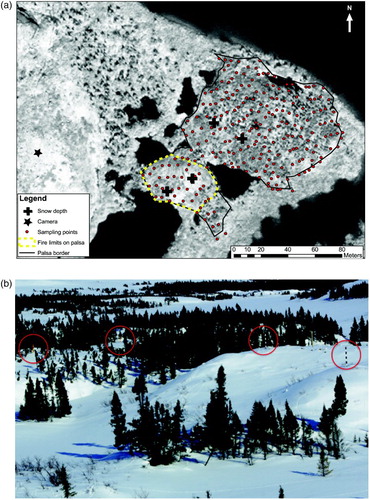
Snow depth measurements were obtained from wooded and non-wooded sections of one particular palsa to assess the sensitivity of the soil temperature regime to vegetation cover. A remote measurement method was implemented based on daily phtotographs of snowstakes. A Pentax K110 camera, controlled by a Digisnap 2000 (Harbortronics®) and fed by two batteries and a 30 W solar panel, was installed on a hill in front of the studied palsa. The system was programmed to take one picture per day, at noon. Four snow stakes were installed on the palsa, two in the forested area, and two in the open area. All stakes were located on the summit of the palsa (Fig. 1) to be visible to the camera. Distance from the snow stakes to the camera was between 100 and 125 m. Accuracy of the measurements is estimated to be between a few centimetres on calm days and up to 10 cm during storms. Three data loggers (HOBOware®, ±0.47°C at 25°C) recorded air temperature every two hours. There was no all-winter precipitation gauge available at the site. All measurements were validated in the field in mid-March 2010.

Fig. 1 (a) Studied palsa on a 2008 Worldview-1 satellite image. The black line represents the limits of the palsa, and the yellow dashed line delineates the open area. The position of the camera is identified by the star symbol. Snow rulers are indicated by the crosses. (b) Example of photos taken by the remote-controlled camera. Snow rulers are shown in the red circles. Photographs courtesy of Mélanie Jean.

The location of the snow rulers on the summit of the palsa likely led to an increased contrast in snow depth between the wooded and non-wooded sites as a result of the higher potential for snow ablation on the exposed summit of the non-wooded site. Typically, snow surveys aimed at estimating average snow depth over an area would avoid overrepresenting such locations. In ecological studies such as this one, monitoring locations are dictated by the objectives of the project.

Several technical problems were encountered, producing some large gaps in the record. In particular, erroneous programming of the Digisnap 2000 led to missing values between October 2009 and February 2010. During the following winter, solar power was insufficient for the camera to function continuously, leading to missing values between December 2010 and February 2011. Missing values were also caused by snowstorms that reduced visibility, humidity infiltration, and snow accumulation on the camera window.

3 Snow depth prediction with empirical snow redistribution

Brown et al. (2003) used a simple degree-day model to obtain monthly snow depth estimates for North America, which has recently been shown to perform well in the Arctic basin (Brown, Derksen, & Wang, 2010). In particular, it is still used by Environment Canada to obtain the initial snow depth for all operational numerical weather forecasting systems at scales of 2.5 to 60 km.

This model requires only daily temperature and precipitation forcings and runs with hourly time steps. Many of its parameters depend on the snow–climate zone to which the modelled location belongs: tundra, taiga, maritime, ephemeral, prairie, alpine, or ice. The fraction of precipitation occurring as snow is diagnosed from temperature. Brown et al. (2003) assume this fraction to be 1.0 for air temperatures of 0°C or less and let it decrease linearly between 0°C and 2°C. A simpler approach was used for this paper in which the fraction of hourly precipitation falling as snow is either zero or one, depending on whether air temperature is above or below zero.

New snowfall density in the model varies between 68 and 139 kg m⁻³ depending on air temperature. In tundra, prairie, and taiga environments, a fraction τ = 20% of the solid precipitation is removed to approximate losses from sublimation. Melt occurs if the hourly temperature is above a threshold temperature of −1°C and is proportional to the difference between the air temperature and that threshold. The coefficient of proportionality increases linearly with snowpack density, the linear relationship being different for forested and open areas. In forested areas, the melt factor varies from 1.4 to 3.5 mm d⁻¹ °C⁻¹, whereas in open areas it varies from 1.5 to 5.5 mm d⁻¹ °C⁻¹. Additional melt occurs for rain on snow events, based on the heat transferred to the snowpack by the rain.

Empirical functions are used to estimate settling and maturing of the snowpack, which causes an increase in snowpack density between snowfall events. These functions depend on predicted snowpack density, air temperature, and the dominant vegetation class. More details, including all equations, can be found in Brown et al. (2003), but for the purposes of this paper, the model can be considered as a black box that, provided with initial values of snow depth (h _t−1) and snow density (ρ _t−1), as well as hourly rainfall (R _t ), hourly snowfall (S _t ), and hourly temperature (T _t ) forcings, can predict snow depth (h _t ), snow density (ρ _t ) and, hence, SWE for a grid cell at the end of the time step, assuming no snow transport in or out of the grid of vegetation class V, as represented by Eq. (1). In this equation, θ^V corresponds to the vector of model parameters associated with vegetation class V. In practice, the vegetation classes used in the paper are the tundra and taiga environments, which are used, respectively, to represent open and forested areas at the test site. Let θ^O be the parameter vector for the open areas and θ^F the parameter vector for the forested areas, then(1)

For a large grid cell with homogeneous vegetation, elevation, and atmospheric forcings, assuming no net snow transport might be reasonable, but in an open forest environment transport of snow from open areas towards more densely forested areas can be significant and lead to shallower and denser snowpacks in open areas (Kershaw & McCulloch, 2007). Snow transport obviously varies with wind speed (Pomeroy et al., 1993), but as a first step towards taking into account snow transport in a simple degree-day model, it was decided to first try simple, conceptual approaches to snow transport modelling. Two simple mechanisms for transporting snow from open areas to forested areas were, therefore, considered: (i) a mechanism by which a fraction of the falling snow is immediately transported, as it falls, from the open areas to the forested areas and (ii) a mechanism by which a fraction of the snow on the ground above a certain threshold (representing shrub height) is transported from the open areas to the forested areas at each time step. The first approach assumes that most transport occurs shortly after the deposition of fresh snow, before it has time to consolidate. The second approach is only expected to work well in a windy environment where the snow transfer process is more-or-less continuous.

The first process results in snowfall being different for open and forested areas and is modelled by Eq. (2), which is referred to later in the paper as Model 1. Two additional parameters are required: α _S  represents the fraction of the snowfall which is immediately transported from the open area to the forested area, and represents the effect this transport of snow has on snowfall in the forested area. If the model is expected to represent areal average snow depth and SWE, then conservation of mass implies that should be equal to the ratio of the areal extent of the open environment to the areal extent of the forested environment. For the case in which the model is calibrated on point measurements (and not sampling all sources and sinks), it does not have to be the case. Once the snowfall is adjusted using Eqs (2), the snow model of Brown et al. (2003) is called separately for the open and forested areas (Eqs (3)).(2) (3)

The second process results in snow on the ground being transported from open areas to forested areas and is modelled by Eqs (5), and referred to later as Model 2. Here, represents the snow depth threshold required to trigger snow transport, represents the fraction of the snow depth which can be transported each time step when the snow depth is above the threshold, and represents the sublimation rate, set at as in Brown et al. (2003). The parameter appears once again to reflect the difference in the areal extent of the source and sink areas. Observe that the time index of the snow depth state variable which appears on the right-hand side of Eqs (5) is , to reflect the fact that this step is done after the degree-day snow model has completed its time step (Eqs (4)). Furthermore, not only does snow depth need to be adjusted in this model, but snowpack density does also.(4) (5)

Note that both processes can be combined into a single, more complex model although it would likely be overparameterized for practical applications.

4 Using CaPA for estimating daily snowfall amounts

A large number of continental-scale and global gridded precipitation products have been developed over the last two decades, some based solely on gauge data, others merging gauge data with radar and satellite products or short-term weather forecasts (see for example Xie et al. (2007) for a review of existing products). Few are designed for environmental prediction in northern climates, where reliable gauges are often few and far between, especially for solid precipitation. Some products, such as the Tropical Rainfall Measuring Mission (TRMM) Multi-satellite Precipitation Analysis (TMPA; Huffman et al., 2007) are simply not available for northern latitudes. Others, such as the Precipitation Estimation from Remotely Sensed Information using Artificial Neural Networks (PERSIANN; Hsu & Sorooshian, 2009) or atmospheric reanalyses such as the North American Regional Reanalysis (NARR; Mesinger et al., 2006), do not assimilate any gauge observations over Canada (in the case of NARR, no gauges are assimilated after 2003) (Eum, Dibike, Prowse, & Bonsal, 2014).

Mahfouf et al. (2007) presented a statistical interpolation method, known as CaPA, for estimating 6 h precipitation accumulations in real time at a spatial resolution of approximately 15 km over Canada. The method, developed jointly by the Meteorological Research Division of Environment Canada and the MSC, combines observations of precipitation from gauges with a first guess obtained from MSC's regional deterministic prediction system (RDPS), based on the GEM model (Mailhot et al., 2006). Only gauges which pass a strict quality-control procedure are assimilated. In particular, reports in which significant undercatch is expected, given the observed temperature and wind speed at the gauge, are discarded. This particular configuration of CaPA is referred to by MSC as the regional deterministic precipitation analysis (RDPA). See Fortin and Roy (2011) for more details on its operational configuration.

The use of a background field provided by a numerical weather prediction model was necessary in order for the method to be applicable over a territory like Canada where the density of the precipitation observing network varies widely in space, with most stations located in southern Canada and, in time, more observations being available in summer than in winter. In addition to stations operated by MSC, an increasing number of stations from cooperative networks operated by external partners are assimilated within CaPA. Because a significant number of stations from cooperative networks report only 24 h accumulations, a separate 24 h accumulation product is also provided in addition to the 6 h product.

Verification results obtained using a cross-validation technique showed that the 24 h analysis had a lower bias (Fortin and Roy, 2011). For the purpose of modelling snow accumulation and melt over an entire winter with a degree-day model, it is far more important to avoid bias than to obtain accumulations on time scales shorter than one day, which is why it was decided for this paper to use a 24 h accumulation period. In order to obtain hourly forcings, the temporal structure provided by the GEM precipitation was used, and scaled upward or downward using a multiplicative factor so that the daily totals at 1200 utc would match the analysis. In the rare case when GEM forecasted no precipitation for 24 h and CaPA predicted some, the daily total was simply divided into 24 equal amounts.

Eum et al. (2014) recently evaluated CaPA for hydrological simulation over the Athabasca river watershed and concluded that CaPA “could be a good alternative source of precipitation data for regions with a sparse observational network.” The best results were obtained for the lower portion of the watershed which is at a latitude comparable to Rivière Boniface.

Figure 2 shows an example of the RDPA product obtained with the CaPA system, a 24 h accumulation of precipitation valid on 1 December 2011 at 1200 utc. The red circle shows the location of the Rivière Boniface site. Smaller black dots show the location of the 15 km GEM model grid points on which CaPA relied in 2011. Note that the horizontal resolution of GEM and CaPA was increased to 10 km in October 2012.

Fig. 2 24 h precipitation accumulation from CaPA RDPA valid 1 December 2011 at 1200 utc. The red circle shows the location of the Rivière Boniface site. The black dots show the CaPA grid.

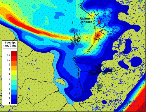
It can be seen that the precipitation taking place at Rivière Boniface is part of an event occuring over Hudson Bay. This is fairly typical for December, a time when the water of Hudson Bay is significantly warmer than the air above, which leads to high evaporation rates over all of Hudson Bay. The moist air mass is then advected east, and condensation occurs rapidly as the air mass moves over land.

5 Calibration and verification of snow depth predictions at Rivière Boniface

Data from 1 October 2009 to 20 June 2010 were used to estimate the parameters of the snow redistribution models presented in Section 3. The parameters were identified by minimizing the sum of squares differences between observed and predicted snow depth, using a systematic search of the parameter space further refined using the Nelder-Mead simplex method, as implemented in MATLAB (Version 7.10.0.499; 2010). The second winter (1 October 2010 to 20 June 2011), was only used to assess model performance.

The parameters obtained for Model 1 are and , which means that snowfall needs to be cut in half at the open site and increased by at the forested site in order to obtain accurate snow depth predictions. The parameters obtained for Model 2 are  cm⁻¹, cm, and , which means that cm of snow can be transported every hour from the open area to the forested site where snow depth is above 11 cm, where it can lead to an increase of up to  cm d⁻¹ of snow at the forested site. A test combining both approaches to snow redistribution in a single model was also carried out. This did not produce any significant improvement in the accuracy of the prediction, even for the calibration period. In fact, the optimal value of was very close to zero; hence, the model parameters were very close to those obtained for Model 2.

Figures 3a and 3b show the results obtained for the winters of 2010 and 2011 with the original snow model of Brown et al. (2003), which treats open and forested areas differently (snow density being higher for the tundra vegetation class than for the taiga class) but without allowing for snow redistribution. It can be seen that this model leads to a deeper snowpack at the forested site (red line) than observed, but the snow depth observed at the open site (blue line) is smaller than observed. Results for Model 1, which redistributes incoming snowfall, are shown in Figs 3c and 3d. Much improved predictions are obtained for both winters. Similar results are obtained with Model 2, as shown in Figs 3e and 3f, which redistributes snow on the ground. Model 2 performs slightly better than Model 1 in terms of root mean square (RMS) error for the first winter, but for the second winter it is outperformed by Model 1 at the forested site (see Table 1).

Fig. 3 Initial model run: (a) winter 2010 and (b) winter 2011. Model 1 (advection of snowfall): (c) winter 2010 and (d) winter 2011. Model 2 (advection of snow on the ground): (d) winter 2010 and (e) winter 2011.

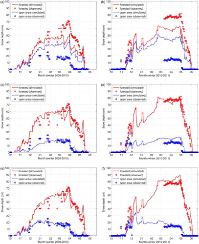
Table 1. Root mean square error (cm) of different snow depth prediction models.

	Winter 2009–2010		Winter 2010–2011
Model configuration	Open area	Forested area	Open area	Forested area
Initial model run	16.4	14.1	19.8	12.9
Model 1	3.2	9.3	5.5	5.6
Model 2	2.6	7.8	3.7	7.4
Model 2 with data assimilation	2.0	4.8	2.6	3.1

Despite the lack of a long-term record of snow depth at this location, it is important to characterize those two years with respect to local climatology. Indeed, calibration and verification periods should be representative of typical conditions encountered in this region for the model to have good general performance, and the verification period should ideally differ significantly from the calibration period in order to present a good prediction test for the model. One source of information on snow depth is the Canadian Meteorological Centre (CMC) real time snow depth analysis (Brasnett, 1999), which is available from 1999 to the present and relies on the same snow accumulation and melt model used in this paper. According to this product, the maximum snow depth at this location was, on average, 48 cm between 1999 and 2014, with a standard deviation of 9 cm. For the winter of 2009/10, the maximum analyzed snow depth was 43 cm, compared with 51 cm for the winter of 2010/11. Hence, the calibration winter saw below average snow depth (by 5 cm or 5/9 standard deviation) whereas the verification winter saw above average snow depth (by 3 cm or 1/3 standard deviation). It is interesting to note that these values compare very well with the simulated maximum annual snow depth for the non-forested area when snow redistribution is not taken into account (blue line in Figs 3a and 3b). The difference between the maximum simulated snow depth and the maximum analyzed snow depth from the CMC analysis was less than 1 cm for both winters.

6 Data assimilation of snow depth observations

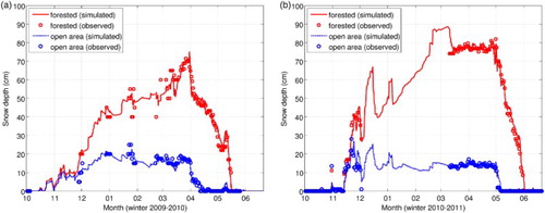
Results presented in Section 5 suggest that a snow model taking into account snow redistribution through a simple empirical parameterization calibrated on one winter season has predictive skill when applied to a subsequent year. Furthermore, Model 2 which redistributes snow on the ground performed better over the calibration period. Even better results can, however, be obtained with Model 2 when it is constrained by past observations using data assimilation.

When observations become available, a simple data assimilation scheme can be used to update the predictions made by the snow model. A fairly simple nudging scheme can be used because only observations for one state variable, snow depth, are available. Furthermore, as can be seen from Fig. 3, when observations are available for a given day, they are available for both the open and the forested site. Hence, it is not necessary to devise a data assimilation strategy which updates the state of the snowpack at both sites based on an observation at a single site.

The simplest data assimilation strategy would consist of replacing the predicted snow depth by the observed snow depth each time an observation becomes available. However, because observations can be noisy, a better approach is to blend the observed and predicted snow depth by using a weighted average of the observed and predicted snow depth. The skill of the prediction will vary as a function of the weight given to observations. One way to assess the skill of this product is to measure the RMS prediction error for the next observation (i.e., the prediction error measured before the update step). This was done for winter 2009/10, but focusing only on observations during the snow accumulation period (October to March) in order to avoid putting too much weight on the snowmelt period for which ample observations were already available, because one purpose of the model is to fill the observation gaps occurring earlier in the season. A weight of 30% for the observations leads to the best results in terms of RMS error. When assessed over the entire season, the reduction in the RMS error is quite significant, especially in the forested area; over the two winters, the error drops, on average, by 1 cm in the open area and by 4 cm in the forested area (see Table 1).

One of the limitations of this simple data assimilation scheme is that the uncertainty in the model parameters is not explicitly taken into account; a single parameter set is used, which corresponds to the parameters giving the best results over the calibration period (Model 2, see Section 5).

Figure 4 shows the predictions obtained with this sequential data assimilation procedure for both winters. Note that the predicted values, which are plotted, correspond to the model prediction before each update step, which explains why large discrepancies can still be observed between the predicted and observed snow depth. By comparing Figs 3c and 3f with Fig. 4, it can be seen that results are improved over most of the season, from the onset of winter to the end of the snowmelt period. This is, however, not always the case. During the winter of 2011, no observations were available for over three months. At the end of this period, in early March of 2011, snow depth predicted in the forested area was close to 90 cm, about 10 cm more than the observations, a model overshoot which is not as important in the open loop simulations. This is fairly typical when sequential data assimilation techniques are used with models having a long-term memory of initial conditions. In this case, better results could potentially be obtained by using a smoothing technique rather than a sequential assimilation technique, in which only past observations are assimilated.

Fig. 4 Model 2 (advection of snow on the ground) with sequential assimilation of snow depth observations: (a) winter 2010 and (b) winter 2011.

7 Discussion and conclusions

Although the impact of vegetation cover on snow depth has long been recognized, many models used for operational environmental prediction applications fail to take into account snow redistribution across the landscape. This is partly because physically based models accounting for snow redistribution require high-resolution atmospheric forcings and geophysical information that exceeds operational constraints. Even when such information is available, ground truthing is required for model calibration. In remote locations, obtaining frequent observations of snow depth is challenging. Time-lapse photography using a digital camera offers a practical solution for monitoring both spatial and temporal variability of snow depth, particularly in Arctic and alpine regions where the lower density of the forest allows for remote observations of snow depth.

Results from a two-year study suggest that relatively simple conceptual models of snow transport can be applied to a temperature index-based snowpack model to provide realistic estimates of snow cover conditions at forested and non-forested sites in the forest-tundra ecotone of northern Quebec. Two algorithms were tested: a simpler model in which only the snowfall input was modified and a slightly more sophisticated approach in which snow on the ground was adjusted at the end of each time step in order to advect snow from the non-forested site to the forested site. The first approach (Model 1) requires no modification to the snow model nor to its driver, because only an input file needs to be modified. The second approach (Model 2) requires changes to the model driver but not to the model itself; the state variables of the model are updated at the end of each time step.

Model parameters were calibrated using data from the first winter, and model performance was assessed using data from the second winter. While the second, more sophisticated model performed better for the first year, it did not outperform the simpler model during the second year. A simple data assimilation scheme was then tested and shown to provide accurate predictions of snow depth at both the non-forested and the forested site, with an RMS error of 2 to 5 cm. In comparison, the initial model runs (without snow redistribution) had an RMS error ranging from 13 to 20 cm.

Model results and observations suggest that although snowmelt starts at approximately the same time at both the non-forested and forested sites, snow remains on the ground at the forested site for about one month longer. The date at which the maximum accumulation is observed sets the models apart. In the first model, which redistributes snowfall, snow continues to accumulate throughout the winter season at the non-forested site. In the second model, which redistributes snow already on the ground, maximum snow depth is observed early in the season.

The differences in observed and predicted snow depth between the two sites is sufficiently important to warrant caution when using snow depth products derived from a snow model which does not take into account snow redistribution in such an environment. Furthermore, data assimilation could make matters worse. Indeed, if observations being assimilated are biased towards non-forested (forested) areas, the resulting single model prediction will underpredict (overpredict) average conditions, even if the model itself might adequately represent average conditions, as suggested by Figs 3a and 3b. This is the case with the current operational implementation of the daily snow depth analysis issued by Environment Canada.

This study also provides an evaluation of CaPA (RDPS configuration) in northern Canada. Given the challenges involved in accurately measuring snowfall as well as the low density of the observing network, it is very difficult to verify CaPA products in winter. Results obtained suggest that CaPA has sufficient skill to drive a snow accumulation and melt model in this region in near real time. However, large-scale application of such a snow model in the forest–tundra ecotone would require that parameters be estimated from existing geophysical data. Given the similar skill level obtained with both snow redistribution strategies tested in this paper, Model 1, which has only two parameters and can be implemented by changing only the inputs to the snow model, could be tested first. The parameter could be set to the ratio of the areal extent of the open environment to the areal extent of the forested environment, leaving only one free parameter, This parameter could be adjusted in order that the annual maximum snow depth at the non-forested site corresponds approximately to shrub height. Indeed, shrubs are known to trap snow and also to have their growth limited by snow depth because exposed tissues are subject to additional risk of mechanical breakage and desiccation during winter (Sturm et al., 2001). As a consequence, this parameter would likely need to evolve with time, because a recent expansion and densification of shrub cover has been documented in the forest–tundra ecotone (Ropars & Boudreau, 2012).

Attempting to map snow depth across the forest–tundra ecotone while taking into account snow redistribution is a challenge well beyond the scope of this paper. Research efforts should, at this point, be focused on obtaining similar datasets at other locations to better ground the parameter estimation procedure for a large-scale application of the model, either through time-lapse photography or other means of monitoring snow depth in both non-forested and forested areas of the forest–tundra ecotone.

A more convincing argument for the snow depth modelling approach proposed in this paper could be made if SWE datasets could also be obtained. The ongoing World Meteorological Organization Solid Precipitation Intercomparison Experiment (SPICE) project (Nitu, 2013), and its companion project C-SPICE (Canadian SPICE), provide new opportunities to access high-quality snow data in northern environments, including the forest–tundra ecotone. This avenue will be explored in order to further calibrate and validate the snow redistribution scheme at various SPICE and C-SPICE locations, in particular Caribou Creek in northern Saskatchewan.

Although the approaches tested in this paper for snow redistribution performed well for the purpose of predicting snow depth, the snow redistribution processes are very much conceptual, as is the snow accumulation and melt model used as the starting point for the study. It would certainly be interesting to compare the skill of the model to a more physically based snow model allowing for snow redistribution, such as the parameterizations proposed by MacDonald, Pomeroy, & Pietroniro (2009) and Dornes, Pomeroy, Pietroniro, Carey, & Quinton (2008). Perhaps an intermediate approach in terms of complexity, relying on a simple degree-day model for snow accumulation and melt but in which the snow redistribution and sublimation rates depend on wind speed as in Turcotte et al. (2010), would suffice.

However, even in its current state, the proposed model could be tested at a larger scale, given that it does not require any more meteorological inputs than the original snow model of Brown et al. (2003) and can be forced by CaPA, which is available for all of North America. In particular, possible impacts on weather forecasts initialized during the snow melt period should be investigated.

Finally, the data assimilation procedure could also be improved by taking into account model error (both parameter and structural uncertainty) and by using a smoothing rather than a filtering method, in order to be able to use both past and future observations when assessing snow depth at a given instant in time. This would also allow for the development of probabilistic predictions of snow depth, in which predictions would be provided together with an associated credibility interval that would reflect the impact of data assimilation on the reduction of model error. Despite the limitations of the model and of the data assimilation procedure, the predictive skill obtained when assimilating observations of snow depth from time-lapse photography suggests that digital cameras and snow stakes should be considered for inclusion in the set of instruments deployed at weather and climate stations across Canada's North.

Acknowledgements

We wish to acknowledge the contribution of Guy Roy, Meteorological Service of Canada, and Franck Lespinas, University of Manitoba, for their support in providing the CaPA precipitation dataset used in this study. We also wish to thank the Fonds de recherche du Québec Nature et technologies (FQRNT) as well as the Natural Sciences and Engineering Research Council of Canada (NSERC) for their financial support. Logistical support was provided by the Centre d’études nordiques (CEN).

Disclosure statement

No potential conflict of interest was reported by the authors

References

- ACGR-NRC (Associate Committee on Geotechnical Research-National Research Council) (1988). Glossary of permafrost and related ground ice terms. Ottawa, ON: Associate Committee on Geotechnical Research, Permafrost Subcommittee, National Research Council of Canada, Technical Memorandum 142.
- Arseneault, D., & Payette, S. (1997). Landscape change following deforestation at the arctic tree line in Quebec, Canada. Ecology, 78, 693–706.
- Brasnett, B. (1999). A global analysis of snow depth for numerical weather prediction. Journal of Applied Meteorology, 38(6), 726–740. doi: 10.1175/1520-0450(1999)038<0726:AGAOSD>2.0.CO;2
- Brown, R., Brasnett, B., & Robinson, D. (2003). Gridded North American monthly snow depth and snow water equivalent for GCM evaluation. Atmosphere-Ocean, 41, 1–14. doi: 10.3137/ao.410101
- Brown, R., Derksen, C., & Wang, L. (2007). Assessment of spring snow cover duration variability over northern Canada from satellite datasets. Remote Sensing of Environment, 111(2–3), 367–381. doi: 10.1016/j.rse.2006.09.035
- Brown, R., Derksen, C., & Wang, L. (2010). A multi-data set analysis of variability and change in Arctic spring snow cover extent, 1967–2008. Journal of Geophysical Research, 115, D16111. doi:10.1029/2010JD013975
- Burn, C. R., & Koklej, S. V. (2009). The environment and permafrost of the Mackenzie Delta area. Permafrost and Periglacial Processes, 20, 83–105. doi: 10.1002/ppp.655
- Cyr, H., & Payette, S. (2010). The origin and structure of wooded permafrost mounds at the arctic treeline in eastern Canada. Plant Ecology & Diversity, 3(1), 35–46. doi: 10.1080/17550871003777176
- Derksen, C., Walker, A., & Goodison, B. (2003). A comparison of 18 winter seasons of in situ and passive microwave-derived snow water equivalent estimates in Western Canada. Remote Sensing of Environment, 88(3), 271–282. doi:10.1016/j.rse.2003.07.003
- Dornes, P. F., Pomeroy, J. W., Pietroniro, A., Carey, S. K., & Quinton, W. L. (2008). Influence of landscape aggregation in modelling snow-cover ablation and snowmelt runoff in a sub-arctic mountainous environment. Hydrological Sciences Journal, 53(4), 725–740. doi: 10.1623/hysj.53.4.725
- Dutra, E., Balsamo, G., Viterbo, P., Miranda, P. M. A., Beljaars, A., Schar, Ch., & Elder, K. (2010). An improved snow scheme for the ECMWF land surface model: Description and offline validation. Journal of Hydrometeorology, 11, 899–916. doi: 10.1175/2010JHM1249.1
- Eum, H.-I., Dibike, Y., Prowse, T., & Bonsal, B. (2014). Inter-comparison of high-resolution gridded climate data sets and their implication on hydrological model simulation over the Athabasca Watershed, Canada. Hydrological Processes, 28(14), 4250–4271. doi: 10.1002/hyp.10236
- Filion, L., & Payette, S. (1982). Regime nival et vegetation chionophile a Poste-de-la-Baleine, Nouveau-Québec. Naturaliste Canadien, 109, 557–571.
- Fortin, V., & Roy, G. (2011). The Regional Deterministic Precipitation Analysis (RDPA). Environment Canada, technical note dated 2011–04-04, Retrieved from http://collaboration.cmc.ec.gc.ca/cmc/cmoi/product_guide/submenus/capa_e.html
- Fortin, V., Therrien, Ch., & Anctil, F. (2008). Correcting wind-induced bias in solid precipitation measurements in case of limited and uncertain data. Hydrological Processes, 22, 3393–3402. doi: 10.1002/hyp.6959
- French, H. M. (2007). The periglacial environment (3rd ed.). Chichester, UK: Wiley & Sons.
- Goodison, B. E., Louis, P. Y. T., & Yang, D. (1998). WMO solid precipitation measurement intercomparison, final report. World Meteorological Organization instruments and observing methods report no. 67, Retrieved from http://www.wmo.int/pages/prog/www/reports/WMOtd872.pdf
- Hinkler, J., Pedersen, S. B., Rasch, M., & Hansen, B. U. (2002). Automatic snow cover monitoring at high temporal and spatial resolution, using images taken by a standard digital camera. International Journal of Remote Sensing, 23(21), 4669–4682. doi: 10.1080/01431160110113881
- Hsu, K.-L., & Sorooshian, S. (2009). Satellite-based precipitation measurement using PERSIANN system. In S. Sorooshian, K.-I. Hsu, E. Coppola, B. Tomassetti, M. Verdecchia, & G. Visconti (Eds.), Hydrological Modelling and the Water Cycle (pp. 27–48). Springer. Retrieved from http://www.springer.com/earth+sciences+and+geography/hydrogeology/book/978-3-540-77842-4
- Huffman, G. J., Bolvin, D. T., Nelkin, E. J., Wolff, D. B., Adler, R. F., Gu, G., … Stocker, E. F. (2007). The TRMM Multisatellite Precipitation Analysis (TMPA): Quasi-global, multiyear, combined-sensor precipitation estimates at fine scales. Journal of Hydrometeorology, 8, 38–55. doi: 10.1175/JHM560.1
- Jean, M., & Payette, S. (2014a). Dynamics of active layer in wooded palsas of northern Quebec. Geomorphology, 206, 87–96. doi: 10.1016/j.geomorph.2013.10.001
- Jean, M., & Payette, S. (2014b). Effect of vegetation cover on the ground thermal regime of wooded and non-wooded palsas. Permafrost and Periglacial Processes, 25(4), 281–294. doi: 10.1002/ppp.1817
- Kershaw, G. P., & McCulloch, J. (2007). Winter snowpack variation across the Arctic treeline, Churchill, Manitoba, Canada. Arctic, Antarctic and Alpine Research, 39, 9–15. doi: 10.1657/1523-0430(2007)39[9:MSVATA]2.0.CO;2
- Liston, G. E., & Sturm, M. (1998). A snow-transport model for complex terrain. Journal of Glaciology, 44, 498–516.
- MacDonald, M. K., Pomeroy, J. W., & Pietroniro, A. (2009). Parameterizing redistribution and sublimation of blowing snow for hydrological models: Tests in a mountainous subarctic catchment. Hydrological Processes, 23(18), 2570–2583. doi: 10.1002/hyp.7356
- Mahfouf, J.-F., Brasnett, B., & Gagnon, S. (2007). A Canadian precipitation analysis (CaPA) project: Description and preliminary results. Atmosphere-Ocean, 45(1), 1–17. doi: 10.3137/ao.450101
- Mailhot, J., Belair, S., Lefaivre, L., Bilodeau, B., Desgagne, M., Girard, C., … Qaddouri, A. (2006). The 15-km version of the Canadian regional forecast system. Atmosphere-Ocean, 44(2), 133–149. doi: 10.3137/ao.440202
- MATLAB (Version 7.10.0.499) [Computer Software]. (2010). The Mathworks Inc., Natick, Massachussetts. Retrived from http://www.mathworks.com
- Mesinger, F., DiMego, G., Kalnay, E., Mitchell, K., Shafran, P. C., Ebisuzaki, W., … Shi, W. (2006). North American Regional Reanalysis. Bulletin of the American Meteorological Society, 87(3), 343–360. doi: 10.1175/BAMS-87-3-343
- Nitu, R. (2013). Cold as SPICE: Determining the best way to measure snowfall. Meteorological Technology International, August 2013, 148–150. Retrived from http://viewer.zmags.com/publication/f088b3fc#/f088b3fc/10
- Oreiller, M., Rousseau, A. N., Minville, M., & Nadeau, D. F. (2013). Modelling snow water equivalent and spring runoff in a boreal watershed, James Bay, Canada. Hydrological Processes, 28(25). doi:10.1002/hyp.10091
- Parajka, J., Haas, P., Kimbauer, R., Jansa, J., & Bloschl, G. (2012). Potential of time-lapse photography of snow for hydrological purposes at the small catchment scale. Hydrological Processes, 26(22), 3327–3337. doi:10.1002/hyp.8389
- Payette, S. (1983). The forest tundra and the present tree-lines of the Northern Quebec-Labrador Peninsula. Tree-line Ecology. In P. Morisset & S. Payette (eds.), Proceedings of the Northern Quebec Tree-Line Conference, Centre d'etudes nordiques (pp. 141–151). Quebec, Canada: Universite Laval.
- Pomeroy, J. W., Gray, D. M., & Landine, P. G. (1993). The prairie blowing snow model: Characteristics, validation, operation. Journal of Hydrology, 144, 165–192. doi: 10.1016/0022-1694(93)90171-5
- Roche, Y., & Allard, M. (1996). L'enneigement et la dynamique du pergelisol: l'exemple du detroit de Manitounuk, Quebec nordique. Geographie Physique et Quaternaire, 50(3), 377–393. doi: 10.7202/033107ar
- Ropars, P., & Boudreau, S. (2012). Shrub expansion at the forest-tundra ecotone: Spatial heterogeneity linked to local topography. Environmental Research Letters, 7(1). doi: 10.1088/1748-9326/7/1/015501
- Seppala, M. (1972). The term “palsa”. Zeitschrift für Geomorphologie N.F., 16, 463.
- Singh, M., Mishra, V. D., Thakur, N. K., Kulkarni, A. V., & Singh, M. (2009). Impact of climatic parameters on statistical stream flow sensitivity analysis for hydro power. Journal of the Indian Society of Remote Sensing, 37, 601–614. doi: 10.1007/s12524-009-0053-3
- Stieglitz, M., Dery, S. J., Romanovsky, V. E., & Osterkamp, T. E. (2003). The role of snow cover in the warming of arctic permafrost. Geophysical Research Letters, 30(13), 1721. doi:10.1029/2003GL017337
- Sturm, M., Holmgren, J., McFadden, J. P., Liston, G. E., Chapin, F. S., & Racine, C. H. (2001). Snow-shrub interactions in Arctic tundra: A hypothesis with climatic implications. J. Climate, 14, 336–344. doi: 10.1175/1520-0442(2001)014<0336:SSIIAT>2.0.CO;2
- Todhunter, P. E. (2001). A hydroclimatological analysis of the Red River of the North snowmelt flood catastrophe of 1997. Journal of the American Water Resources Association, 37(5), 1263–1278. doi: 10.1111/j.1752-1688.2001.tb03637.x
- Turcotte, R., Fortier Filion, T.-C., Lacombe, P., Fortin, V., Roy, A., & Royer, A. (2010). Simulation hydrologique des derniers jours de la crue de printemps: le probleme de la neige manquante. Hydrological Sciences Journal, 55(6), 872–882. doi: 10.1080/02626667.2010.503933
- Turcotte, R., Fortin, L.-G., Fortin, V., Fortin, J.-P., & Villeneuve, J.-P. (2007). Operational analysis of the spatial distribution and the temporal evolution of the snowpack water equivalent in southern Quebec, Canada. Nordic Hydrology, 38(3), 211–234. doi: 10.2166/nh.2007.009
- Vajda, A., Venülainen, A., Hanninen, P., & Sutinen, R. (2006). Effect of vegetation on snow cover at the northern timberline: A case study in Finnish Lapland. Siva Fennica, 40(2), 195–207.
- Vallee, S., & Payette, S. (2007). Collapse of permafrost mounds along a subarctic river over the last 100 years (northern Quebec). Geomorphology, 90, 162–170. doi: 10.1016/j.geomorph.2007.01.019
- Varhola, A., Wawerla, J., Weiler, M., Coops, N. C., Bewley, D., & Alila, Y. (2010). A new low-cost, stand-alone sensor system for snow monitoring. Journal of Atmospheric and Oceanic Technology, 27(12), 1973–1978. doi:10.1175/2010JTECHA1508.1
- Walter, M. T., McCool, D. L., King, L. G., Molnau, M., & Campbell, G. S. (2004). Simple snowdrift model for distributed hydrological modeling. Journal of Hydrologic Engineering, 9(4), 280–287. doi: 10.1061/(ASCE)1084-0699(2004)9:4(280)
- Westerling, A. L., Hidalgo, H. G., Cayan, D. R., & Swetnam, T. W. (2006). Warming and earlier spring increase western U.S. forest wildfire activity. Science, 313, 940–943. doi: 10.1126/science.1128834
- Xie, P., Chen, M., Yang, S., Yatagai, A., Hayasaka, T., Fukushima, Y., & Liu, C. (2007). A gauge-based analysis of daily precipitation over East Asia. Journal of Hydrometeorology, 8, 607–626. doi: 10.1175/JHM583.1
- Zoltai, S. C. (1972). Palsas and peat plateaus in central Manitoba and Saskatchewan. Canadian Journal of Forest Research, 2, 291–302. doi: 10.1139/x72-046
- Zoltai, S. C., & Tarnocai, C. (1971). Properties of a wooded palsa in northern Manitoba. Arctic and Alpine Research, 3, 115–129. doi: 10.2307/1549981