Influence of the South China Sea Biweekly Sea Surface Temperature on the South China Sea Summer Monsoon Especially during the Indian Ocean Dipole

ABSTRACT

The influence of the biweekly sea surface temperature (SST) in the South China Sea (SCS) on the SCS summer monsoon, especially during the Indian Ocean Dipole (IOD) is presented using the Tropical Rainfall Measuring Mission (TRMM) Microwave Imager (TMI) SST and rainfall data for April to June from 1999 to 2013. During positive IOD (PIOD) years the biweekly SST anomalies over the SCS lead the rain anomalies by three days, with a significant correlation (r = 0.8, at the 99% confidence level), whereas during negative IOD (NIOD) years, the correlation is only 0.2. The biweekly SST is observed to influence the westward and northward propagating rainfall anomalies over the SCS and, hence, affect the SCS summer monsoon, especially during PIOD years. No such propagation was seen during NIOD years. The biweekly intraseasonal oscillation of SST in the SCS results in enhanced sea level pressure and surface shortwave radiation, especially during PIOD years. The potential findings here indicate that the biweekly SST in the SCS is strongly (weakly) influenced during PIOD (NIOD) years. Further, it is observed that SST in the SCS has a strong (weak) effect on the SCS summer monsoon by westward and northward propagation of rainfall, especially during PIOD (NIOD) years. When a PIOD or NIOD exists over the tropical Indian Ocean, the SCS SST will be strongly (r = 0.6, at the 99% confidence level) or weakly correlated with the residual index, respectively.

RÉSUMé

[Traduit par la rédaction] Nous étudions l'influence de la température bimensuelle de la surface marine (SST), en mer de Chine méridionale, sur la mousson estivale de cette région, notamment, en présence du dipôle de l'océan Indien (IOD), et ce, à l'aide des données de SST issues de l'imageur micro-ondes de la Mission de mesure des précipitations tropicales (TRMM) et des données pluviométriques d'avril à juin, de 1999 à 2013. Durant les années de phase positive de l'IOD (pIOD), les anomalies bimensuelles de la SST dans la mer de Chine méridionale devancent de trois jours les anomalies de quantité de pluie, et ce, avec une corrélation significative (r = 0,8, avec un niveau de confiance de 99%), tandis que durant les années de phase négative (nIOD), la corrélation n'atteint que 0,2. La SST bimensuelle semble influer sur les anomalies de quantité de pluie, qui se déplacent vers l'ouest et le nord, dans la mer de Chine méridionale, et perturbe ainsi la mousson estivale de cette mer, particulièrement durant les phases positives de l'IOD. Ce genre de propagation n'est pas survenu durant les phases négatives de l'IOD. L'oscillation intrasaisonnière bimensuelle de la SST en mer de Chine méridionale entraîne une augmentation de la pression au niveau de la mer et du rayonnement de courtes longueurs d'onde à la surface, notamment durant les phases positives. Cette étude tend à démontrer que la SST bimensuelle de la mer de Chine méridionale est fortement (faiblement) touchée durant les années de phase positive (négative) de l'IOD. De plus, nous observons que la SST de la mer de Chine méridionale exerce un effet considérable (faible) sur la mousson estivale de cette région, déplaçant les chutes de pluie vers l'ouest et le nord, tout particulièrement durant les phases positives (négatives) de l'IOD. Lorsque survient la phase positive ou négative de l'IOD dans la région tropicale de l'océan Indien, les SST de la mer de Chine méridionale seront respectivement fortement (r = 0,6, avec un niveau de confiance de 99%) ou faiblement corrélées avec l'indice résiduel.

KEYWORDS:

• biweekly intraseasonal oscillations
• sea surface temperature
• rainfall
• SCS
• Indian Ocean Dipole

1 Introduction

The South China Sea (SCS) is located between the Pacific and Indian Oceans to the southeast of Asia. It has long been recognized from climatological records that the outbreak of the Asian summer monsoon starts first in the SCS region in the April–May period then gradually propagates westward. Investigations of sea surface temperature (SST) over the SCS are very important because the summer monsoon over East Asia generally starts over the SCS (Wang & Lin, 2002). Thus, investigating temporal SST variability over the SCS region can aid in understanding the influences of SST in the SCS on rainfall over the SCS summer monsoon region. The seasonal transition from winter to summer, which usually occurs in April, May, and June in association with the onset of the Asian monsoon (Hirasawa, Kato, & Takeda, 1995) in East and South Asia is characterized by abrupt changes in general circulation and weather patterns in the region (Murakami & Matsumoto, 1994). The onset of the South Asian monsoon occurs later (Chen & Chen, 1995); therefore, it is very important to study SST over the SCS, especially during April, May, and June. Moreover, it is observed that climate variability in the SCS region is influenced by anomalous states of the tropical Indian Ocean (Xie, Xie, Wang, & Liu, 2003), and anomalous states of the SCS can affect the East and Southeast Asian climate (Roxy & Tanimoto, 2011; Zhou, Tam, Zhou, & Chan, 2010). However, anomalous states of the tropical Indian Ocean associated with intraseasonal variability, especially the biweekly SST oscillation over the SCS, in particular during the Indian Ocean Dipole (IOD), has not yet been examined in the literature.

The biweekly or 10–20 day mode intraseasonal (BWI) oscillation is a major intraseasonal oscillation and the most important component of tropical variation on time scales between day-to-day weather and the Madden–Julian oscillation (MJO; Madden & Julian, 1972). However, knowledge of the propagation of the oscillation is limited, especially in the SCS. An examination of the intraseasonal oscillations based on data from the SCS Monsoon Experiment showed that it influences the maintenance and dissipation of the SCS summer monsoon (Chan, Ai, & Xu, 2002; Zhou & Miller, 2005). Consequently, recognition of its temporal evolution is critical for improving regional intraseasonal weather and climate predictions. Moreover, it is observed that the 10–20 day time scale has a crucial role in modifying the activity of the SCS summer monsoon (Mao & Chan, 2005); thus, studying the BWI oscillation over the SCS is of paramount importance. Moreover, the SCS SST associated with the IOD has yet to be considered in the literature. In the present study, we also focused on SST over the SCS and its association with the IOD. The possible role of the BWI oscillation in the SCS summer monsoon during positive IOD (PIOD) and negative IOD (NIOD) phases is investigated.

The IOD is a coupled ocean–atmosphere phenomenon (Saji, Goswami, Vinayachandran, & Yamagata, 1999; Webster, Moore, Loschnigg, & Leben, 1999) and a PIOD (NIOD) is characterized by negative (positive) SST anomalies in the southeastern equatorial Indian Ocean and positive (negative) SST anomalies in the western equatorial Indian Ocean. There is growing evidence that the atmosphere–ocean interaction during an IOD is specific to the Indian Ocean (Hong, Lu, & Kanamitsu, 2008) and that the IOD affects regional ocean climate. Many studies have examined the influence of the IOD on the East Asian summer monsoon and summer rainfall in China (Ding & Chan, 2005). It has been suggested that different phases of the IOD mode may change the intensity of the South Asian High and the western North Pacific anticyclone in summer and, hence, variations of monsoon-induced rainfall over China (Yuan, Yang, Zhou, & Li, 2008). In addition, recent studies (Cai, Rensch, Cowan, & Hendon, 2012; Weller & Cai, 2013) have shown that there is an asymmetry between PIOD and NIOD events, with PIOD events reducing rainfall over southern Australia significantly more than the increase in rainfall experienced with NIOD events. However, on intraseasonal time scales much less attention has been paid to the role of the IOD on the variability of rainfall over the SCS summer monsoon region. Moreover, the role of the SCS in modulating the SCS summer monsoon during IOD years is still unclear. Previous studies were mostly concerned with atmospheric anomalies and their possible association with rainfall over different regions. It is important to mention that because of the exchange of heat, momentum, and moisture between the Indian and East Asian monsoon systems and the SCS on an intraseasonal time scale (Chen & Chen, 1995; Lau, Wu, & Yang, 1998; Mao & Chan, 2005), it is imperative that the SCS intraseasonal anomaly during an IOD be investigated. The present study investigates the hypothesis that SST variation in the SCS affects regional precipitation in two different ways depending on the phase of the IOD.

For that purpose, we examine a suite of new high-resolution satellite observations of SST and precipitation, in addition to an objective analysis of latent heat and shortwave fluxes. The fact that these high quality datasets are available for the last 13 years (since 1999) helps quantify the correlation between the IOD and the SCS thermal states, thus improving confidence in the present results. In this observational study data from 1999 to 2013 are used to gain new insights into how the IOD is associated with SSTs in the SCS, as well as how SSTs in the SCS affect the SCS summer monsoon, especially during late spring and early summer. We focus on biweekly SST oscillations in the SCS during different IOD events. The statistical significance of the surface sensible and latent heat fluxes over the SCS associated with SST over the SCS during an IOD is analyzed. Efforts are made to understand how SST in the SCS contributes to rainfall during the SCS summer monsoon, especially during PIOD years, by considering the interactions of different atmosphere–ocean oscillations on a biweekly time scale. Apart from the effect of the BWI SST oscillation in the SCS on the SCS summer monsoon, we provide an analysis of the ocean–atmosphere interaction involved. To the best of our knowledge, neither of these issues has been previously examined, yet they are important to the understanding of SST in the SCS, especially during IOD years. In Section 2, we describe the data and the basic analysis methods. In Section 3, we begin by demonstrating the connection between the BWI SST of the SCS and the SCS summer monsoon and continue to describe, in more detail, the westward and northward propagation of the BWI during IOD years. We present concluding remarks in Section 4.

2 Datasets and methods

The Tropical Rainfall Measuring Mission (TRMM) Microwave Imager (TMI) provided observations of tropical SST unaffected by clouds, aerosols, or atmospheric water vapour (Wentz, Gentemann, Smith, & Chelton, 2000). The TMI reveals intraseasonal SST perturbations considerably larger in amplitude than provided by the Reynolds SST product (Vaid, Gnanaseelan, & Kumar, 2011; Vecchi & Harrison, 2002). The Version-4 TMI SST and rainfall data can be retrieved from http://www.ssmi.com/. Our study uses three-day running means that have better spatial coverage than the daily data. The original data on 0.25° x 0.25° latitude–longitude grids were interpolated onto 1° x 1° latitude–longitude grids with spatial averaging to reduce missing data. Sea level pressure datasets were obtained from the National Centers for Environmental Prediction-Department of Energy (NCEP-DOE) Reanalysis 2 (Kanamitsu et al., 2002). The surface shortwave radiation flux (SWRF), surface latent heat flux (SLHF), and surface sensible heat flux (SSHF) were obtained at a 1° x 1° resolution with a temporal resolution of one day from the Objectively Analyzed atmosphere–ocean heat fluxes (OAFlux) project (Yu, Jin, & Weller, 2008).

The Lanczos filter (Duchon, 1979) is based on a discrete Fourier transform and is used throughout this study to select the part of the variability spectrum relevant to the phenomenon being focused on. It is a Fourier method of filtering digital data and has also been used successfully by Vaid et al. (2011). To extract the BWI, a Lanczos band-pass filter with cut-off periods of 10 and 20 days and 53 weights was applied to all datasets mentioned above. The 53 daily weights were observed to provide very sharp response cut-offs with negligible Gibbs oscillation.

To understand the role of the IOD in modulating the SCS SST variability, the composite (or mean of the selected years) analysis was calculated for PIOD and NIOD. It is well known that El Niño–Southern Oscillation (ENSO) events are related to the IOD (Cai et al., 2012; Luo et al., 2010; Vaid, Gnanaseelan, & Polito, 2007). To isolate ENSO effects, we removed the linear projection of the Niño 3.4 index onto the Dipole Mode Index (DMI) from the DMI, to obtain a residual index (or DMI|_{Niño3.4 removed}). More specifically, we defined ε as the residual index (i.e., DMI|_{Niño3.4 removed}), X(t) = (x₁ , …, x_n) as the DMI index, Y(t) = (y₁ , …, y_n) as the Niño 3.4 index, both as a function of time t, such that:

The values of α and β are obtained by applying the least squares method using the formula below.

Here the carets on α and β indicate that they are the linear fit estimations of the theoretical parameters α and β. Saji et al. (1999) defined the DMI as the difference in the regional mean SST anomalies (SSTAs) along the equator between the western Indian Ocean (50°E–70°E, 10°S–10°N) and the eastern Indian Ocean (90°E–110°E, 10°S–0°), and it is computed similarly here. The Niño 3.4 index is the area average of SSTAs over the region defined by 5°N–5°S, 170°W–120°W.

The positive and negative DMIs represent the PIOD and NIOD, respectively. It is worth noting that the PIOD years during the study period (1999–2013) are 2006, 2008, and 2012, and the NIOD years are 2005 and 2010. Composites for the following years were prepared for the detailed analysis: 2006, 2008, and 2012, hereafter PIOD years; composites for 2005 and 2010, hereafter NIOD years. Although we used the longest observational time series comprising consistent and simultaneous measurements of SST and precipitation, the total number of independent PIOD and NIOD years is rather small from a statistical standpoint. Caution should be exercised because the results and consequent conclusions are inevitably limited by this fact. Improvement of the statistical robustness of the results would demand a longer time series, and this is addressed in Section 4.

3 Results

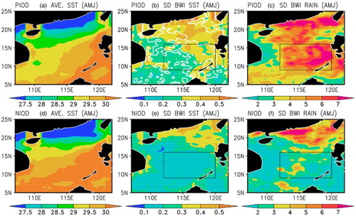
Analysis of the TRMM TMI data for the 1999–2013 period reveals that the mean SST during April, May, and June (AMJ) of PIOD and NIOD years is above 27°C (Figs 1a and 1b), which is conducive to enhanced convective precipitation (Lau, Wu, & Bony, 1997) and is of paramount importance. The regions enclosed by white contours show that the average standard deviation within the box in Fig. 1b is statistically distinct from zero, at the 99% confidence level, from that in Fig. 1e. Therefore, it is clearly evident that in the rectangular box marked in Fig. 1 substantial differences in the variability of the BWI are observed during AMJ of different PIOD and NIOD years. The study demonstrates that the two types of IOD have different features with respect to the impact of their positive and negative phases on SST in the SCS. The different responses are likely linked to the different spatial patterns of the PIOD and NIOD. This was the motivation to investigate the BWI during different IOD years. Strong (weak) biweekly fluctuations in SST (Figs 1b and 1e) and rainfall (Figs 1c and 1f) over the region bounded by 112^oE–120^oE and 9°–16°N (hereafter, Region 1) are observed during PIOD (NIOD) years. Moreover, the selection of Region 1 will be helpful in obtaining a better understanding of the intraseasonal anomalies along with the evolution of the SSTAs, as well as any associated propagation of the biweekly anomalies northward and westward. In our study, we examined the development and maintenance of BWIs over the inset rectangle (Region 1) in Fig. 1, especially during AMJ of PIOD and NIOD years. Strong (weak) biweekly variability in SST and rain during PIOD (NIOD) years indicates that during PIOD years SCS SST is highly correlated, whereas during NIOD years it is not. Also, the biweekly evolution of the SSTAs, as well as its association with the propagation of intraseasonal anomalies, was also investigated during different IOD years. Further, significant strong (weak) biweekly fluctuations in SST and rainfall over Region 1 seem to be associated with ocean–atmosphere processes as discussed later in this article.

Fig. 1 (a) Averaged SST (°C) over the SCS during AMJ PIOD; (b) standard deviation of BWI SST oscillations during AMJ PIOD; (c) standard deviation of BWI rainfall oscillations (mm h⁻¹) during AMJ PIOD; (d) averaged SST (°C) over the SCS during AMJ NIOD; (e) standard deviation of SST BWI oscillations during AMJ NIOD; and (f) standard deviation of BWI rainfall oscillations during AMJ NIOD. The regions enclosed by white contours show that the average standard deviation within the box in (b) is statistically distinct from zero at the 99% confidence level from that in (e), according to the Student's t-test.

To elucidate the ocean–atmosphere interactions, the lead-lag correlations of the biweekly filtered SST and precipitation anomalies over Region 1 are estimated from eight days before to eight days after, for the 15-year period (Fig. 2) during different IOD years. During PIOD years, a positive correlation is observed when SST leads the rainfall indicating that the biweekly SST is driving the atmosphere, which is denoted as an ocean–atmosphere effect. A negative correlation, when biweekly SST lags the biweekly rainfall implies that the atmosphere is driving the SST, which is denoted as an atmosphere–ocean effect. The correlation is not statistically significant (r = 0.11) when the biweekly SST and rainfall are correlated with a 0 lag (Fig. 2). This indicates that the biweekly SST–rain relationship is not an instantaneous one, but has a lead or lag of several days. The maximum positive correlation (r = 0.8, at the 99% confidence level) is observed when SST leads precipitation by three days (Fig. 2). This suggests that ocean–atmosphere processes induced by the intraseasonal SST result in enhanced rainfall during the AMJ period. Whereas, during NIOD years, as already mentioned, a positive correlation that is not statistically significant (r = 0.2) is observed when SST leads precipitation by three days. This shows that biweekly SST and rainfall over the SCS is strongly (weakly) correlated, especially during AMJ of PIOD (NIOD) years. In addition, we tested whether this correlation is specific to the biweekly spectral band or whether it would work at longer time scales. For that, we estimated the lead-lag correlation using the monthly variations of the IOD SST and the SCS SST. No significant correlation was observed in this case.

Fig. 2 The lead-lag correlation between the time series of BWI SST oscillations and rainfall over the rectangular box given in Fig. 1 during AMJ PIOD (solid line) and AMJ NIOD (dashed line). The correlation coefficient is statistically significant at the 99% confidence level.

To investigate the BWI of SST and the associated atmosphere–ocean interaction over the rectangular box drawn in Fig. 1, the time series of the BWI oscillation of key variables were averaged over the inset rectangle in Fig. 1. These are presented in Fig. 3 for the PIOD (left column) and NIOD (right column), both during AMJ. These variables are SST (Figs 3a and 3b), rainfall (Figs 3c and 3d), sea level pressure (SLP) (Figs 3e and 3f), SWRF (Figs 3g and 3h)), SLHF (Figs 3i and 3j), and SSHF (Figs 3k and 3l). It is evident that ocean–atmosphere processes induced by the intraseasonal SST result in enhanced SLP and SWRF during AMJ. Furthermore, it is clearly seen from Fig. 3 that a strong BWI oscillation is predominant during April and May of PIOD years. Interestingly, no such oscillation is evident in NIOD years. We may speculate that the strong biweekly SST oscillation especially during April and May of PIOD years will have a measurable effect on the SCS summer monsoon; this is clearly evident in Table 1.

Fig. 3 BWI time series of (a) SST (°C), (c) Rainfall (mm h⁻¹), (e) SLP (hPa), (g) SWRF (W m⁻²), (i) SLHF (W m⁻²), and (k) SSHF (W m⁻²) averaged over the inset rectangle in Fig. 1 during AMJ PIOD and (b) SST (°C), (d) Rainfall (mm h⁻¹), (f) SLP (hPa), (h) SWRF (W m⁻²), (j) SLHF (W m⁻²), and (l) SSHF (W m⁻²) averaged over the inset rectangle in Fig. 1 during AMJ in NIOD years.

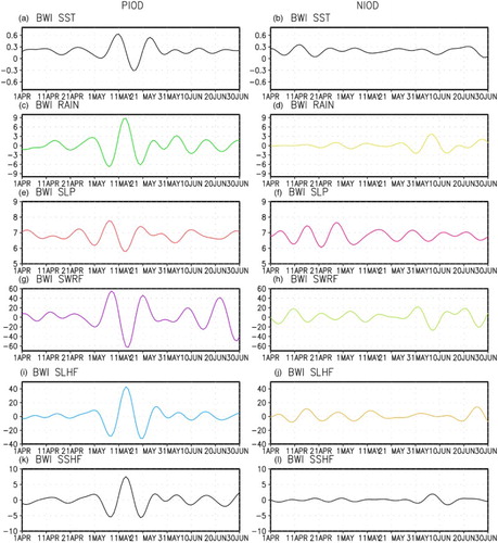
Table 1. Correlation coefficients calculated for PIOD years that are statistically significant at the 99% confidence level. NIOD years yielded no significant correlations. The numbers in bold font shows the biweekly ocean–atmosphere processes induced by the intraseasonal SST which results in enhanced SLP and SWRF with a three-day lag.

Lag (days)	SST and SLHF	SST and SLP	SST and SSHF	SST and SWRF
0	−0.05	0.09	0.00	0.24
1	−0.47	0.41	−0.41	0.55
2	−0.80	0.68	−0.75	0.75
3	−0.95	0.82	−0.93	0.79
4	−0.91	0.81	−0.92	0.68
5	−0.68	0.62	−0.72	0.43
6	−0.33	0.31	−0.39	0.11

In addition, it is evident from Fig. 3 that biweekly SST changes (Fig. 3a) are closely related to surface heat flux anomalies (Figs 3g, 3i, and 3k), and biweekly SST leads biweekly surface SLHF and SSHF. This is taken as an indication that SST is driving the atmosphere, which is denoted as an ocean–atmosphere effect. This suggests that during PIOD years ocean–atmosphere processes induced by the intraseasonal SST result in enhanced SLHFs and SSHFs over the SCS. In addition, it could be speculated that these strong biweekly SST oscillations that peak during April and May of PIOD years have an effect on the onset of the SCS summer monsoon. To study this onset during different IOD years, we analyzed 850 hPa zonal winds over the central and southern part of the SCS (110°–120°E, 5°–15°N). This area was chosen because it was previously used for studying the onset of the summer monsoon over the SCS because it reflects the migration of the subtropical high into and out of the SCS (Li & Mu, 1999; So & Chan, 1997). The onset pentad is defined as the first pentad after mid-April when the five-day mean value of the 850 hPa zonal winds is westerly over the central and southern parts of the SCS and lasts for more than two pentads (Wang et al., 2004b). As far as onset of the SCS summer monsoon during PIOD and NIOD years is concerned, the 850 hPa zonal winds pattern over the SCS (110°–120°E, 5°–15°N) clearly reveals an early onset during PIOD years in contrast to NIOD years (Fig. 4).

Fig. 4 850 hPa zonal winds over the central and southern part of the SCS (110°–120°E, 5°–15°N) during (a) PIOD years and (b) NIOD years.

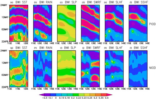
Modelling studies by Kemball-Cook and Wang (2001) and Fu, Yang, Bao, and Wang (2008) demonstrated that atmosphere–ocean coupling on intraseasonal time scales can improve the intraseasonal oscillation phase and propagation, suggesting the importance of atmosphere–ocean interaction to intraseasonal oscillation dynamics. Because of the crucial role (meteorologically, the Indian and East Asian monsoon systems interact over the SCS region) played by the SCS intraseasonal anomalies during the East Asian summer monsoon (Chen & Chen, 1995; Lau et al., 1998; Mao & Chan, 2005), it is imperative that the role played by the SCS intraseasonal anomaly in influencing the SCS summer monsoon intraseasonal anomalies, that is in the 10–20 day time scales, during the entire study period be investigated. Therefore, in the present study, we intended to investigate the role of biweekly SST oscillations in the SCS summer monsoon particularly in PIOD years. To explore this, BWI oscillations are plotted in Fig. 5 for (a) SST (b) RAIN (c) SLP (d) SWRF (e) SLHF (f) SSHF averaged over 9°N–16°N. The top panels of Fig. 5 represent propagation during PIOD years, and the bottom panels represent the signal during NIOD years. Westward propagation over the SCS during April and May of PIOD years can be interpreted as a response to the intraseasonal SST oscillations within the 10–20 day time scale. However, no such propagation was evident during NIOD years. Thus, using satellite observations with a high temporal resolution we presented the evidence that biweekly SST pulses over the SCS are associated with atmosphere–ocean interactions and play a very important role in the variability of the SCS summer monsoon, especially during PIOD years. In addition, it is evident from Fig. 5 that biweekly changes in surface heat fluxes, associated with shortwave radiation changes, induce large SST fluctuations in the SCS and these SST changes could contribute to the westward propagation of rainfall during PIOD years.

Fig. 5 BWI oscillations (a) SST (°C), (b) Rainfall (mm h⁻¹), (c) SLP (hPa), (d) SWRF (W m⁻²), (e) SLHF (W m⁻²), and (f) SSHF (W m⁻²) over 9°–16°N. In order to make the colour bar symmetrical, the values for Rainfall were divided by 10, SLP by 30, SWRF by 50, SLHF by 50, and SSHF by 10.

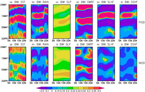
As noted earlier, the phase relationship between SST and rainfall anomalies suggests a role for ocean–atmosphere interaction in the propagation of biweekly anomalies. Latitude-time plots of daily composite variables averaged over the 112°–120°E region are shown in Fig. 6. The top (bottom) panels of Fig. 6 represent signals during PIOD (NIOD) years. Consistent northward migration of SST, Rainfall, SLP, SWRF, SLHF, and SSHF anomalies over the SCS are observed, especially during PIOD years, whereas no such propagation is observed during NIOD years. The biweekly intraseasonal oscillation in SCS SST results in enhanced SLP and surface shortwave radiation, especially during PIOD years. From Figs 5 and 6, the contribution of SCS SST to the westward and northward propagation of biweekly rainfall anomalies during PIOD years is evident, whereas during NIOD years no such propagation is seen. Therefore, we can say that the SCS SST contributes to the westward and northward propagation of biweekly rainfall anomalies during the SCS summer monsoon during PIOD years.

Fig. 6 BWI oscillations (a) SST (°C), (b) Rainfall (mm h⁻¹), (c) SLP (hPa), (d) SWRF (W m⁻²), (e) SLHF (W m⁻²), and (f) SSHF (W m⁻²) over 112°–120°E. Colour bar as in Fig. 5.

To further explore this, the BWI time series of SST averaged over the inset rectangle in Fig. 1 was correlated with rainfall over the region shown in Fig. 7, during AMJ in PIOD years and NIOD years. The correlation coefficient values over Region 1 in Fig. 7 are consistent with those in Fig. 2. It is clearly evident that biweekly SST oscillations have a strong (weak) effect on the SCS summer monsoon region, especially during PIOD (NIOD) years. The westward and northward propagation of rainfall (Figs 5 and 6) purportedly causes the SCS summer monsoon region to receive more rainfall, especially during April and May of PIOD years when BWIs are predominant, as shown in Fig. 3. To examine the effect of the IOD on biweekly SCS SST, the lead-lag correlation between the time series of BWI SST oscillations over the rectangular box given in Fig. 1 and the residual index during AMJ in PIOD years (solid line) and AMJ in NIOD years (dashed line) is shown in Fig. 8. In Fig. 8 the SCS SST during AMJ in PIOD and NIOD years is correlated with DMI|_{Niño3.4 removed} computed during AMJ in PIOD and NIOD years. Interestingly, the DMI|_{Niño3.4 removed} is correlated with the SCS SST only during PIOD years (r = 0.6, at the 99% confidence level), whereas, during NIOD years the correlation between DMI|_{Niño3.4 removed} and the SCS SST is not significant, which shows that the PIOD (NIOD) has a strong (weak) influence on biweekly SST over the SCS. In order to explore the teleconnection of IOD with SCS biweekly SST, wind, and outgoing longwave radiation data were analyzed, and it was observed that IOD does affect the SCS SST (Fig. 9) through distinct wind patterns. Biweekly wind vectors at 850, 500, and 200 hPa during PIOD and NIOD years were regressed (the regression coefficient is statistically significant at the 99% confidence level) onto the residual index (DMI|_{Niño3.4 removed}), which clearly shows the distinct wind vector patterns corresponding to different phases of the IOD (Fig. 9). Thus, PIOD years are observed to be associated with winds from the equator (where convection can be seen prominently; Fig. 10) towards the SCS. Biweekly outgoing longwave radiation during PIOD and NIOD years were regressed (regression coefficient is statistically significant at the 99% confidence level) onto the residual index (DMI|_{Niño3.4 removed}), and it clearly reveals that during PIOD years a convection pattern can be seen over the equator (Fig. 10).

Fig. 7 BWI time series of SST averaged over the inset rectangle in Fig. 1 correlated with rainfall over the domain shown during (a) AMJ PIOD and (b) AMJ NIOD. The correlation coefficient is statistically significant at the 99% confidence level.

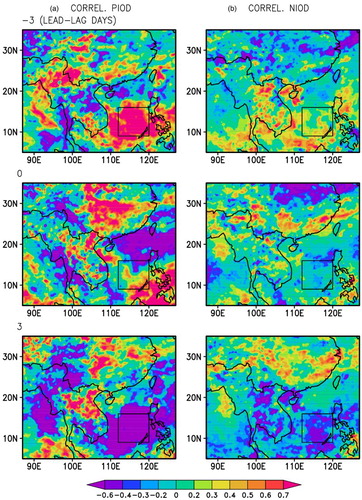
Fig. 8 The lead-lag correlation between the time series of BWI SST oscillations over the rectangular box given in the Fig. 1 and DMI|_{Niño3.4 removed} during AMJ PIOD (solid line) and AMJ NIOD (dashed line). The correlation coefficient is statistically significant at the 99% confidence level.

Fig. 9 Biweekly wind vectors (m s⁻¹) at 850, 500, and 200 hPa during (top panels) PIOD and (bottom panels) NIOD years are regressed (regression coefficient is statistically significant at the 99% confidence level) onto the residual index (DMI|_{Niño3.4 removed}).

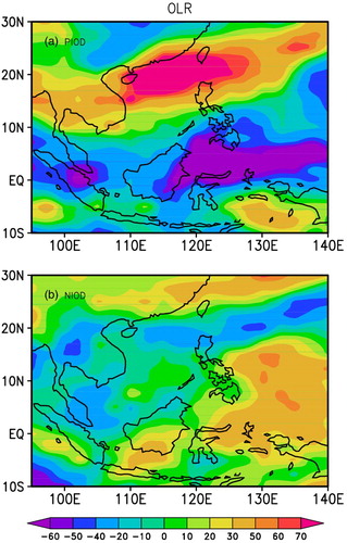
Fig. 10 Biweekly outgoing longwave radiation during PIOD and NIOD years are regressed (regression coefficient is statistically significant at the 99% confidence level) onto the residual index (DMI|_{Niño3.4 removed}).

4 Conclusions

The association of the BWI oscillation in SST and rainfall over the SCS is obtained using Version-4 TMI data during late spring and early summer (AMJ 1999–2013). Our results are novel in that they show that BWIs of the SCS SST anomaly affect the SCS summer monsoon differently during PIOD and NIOD phases. The results suggest that the SCS involves ocean–atmosphere coupling on biweekly time scales which is observed to be very strong (weak) during PIOD (NIOD) events. The biweekly SSTAs lead the rain anomalies over the SCS by three days, with a significant positive correlation (r = 0.8, at the 99% significant level) between the SST and rainfall anomalies during PIOD events, whereas during NIOD events the correlation is only 0.2. Our study suggests that ocean–atmosphere processes induced by BWI oscillations in the SCS SST results in enhanced SLP and surface shortwave radiation flux, especially during AMJ of PIOD years. The SCS SST influences rainfall variability during the SCS summer monsoon via westward and northward propagation of rainfall during PIOD years, whereas during NIOD years such propagation was absent (Figs 5 and 6). The relationship between the SCS summer monsoon and the SCS SST is stronger during PIOD years, whereas the relationship between the SCS summer monsoon and SST in the SCS is weak during NIOD years (Fig. 7). The PIOD has a significant positive influence on SCS SST, whereas the NIOD does not have a significant influence. The different response is likely linked to the different spatial patterns of the PIOD and NIOD. The IOD is observed to be strongly correlated with the SCS SSTs during PIOD years (r = 0.6, at the 99% confidence level) but weakly correlated during NIOD years (correlation not significant). No previous studies have shown an association between the IOD and the role of SST in the SCS in influencing the SCS summer monsoon, especially during PIOD years.

The current skill of most atmospheric general circulation models is poor in predicting the Asian summer monsoon because of their sensitivity to intraseasonal variability (Goswami, Guoxiong, & Yasunari, 2006; Kang, Lee, & Park, 2004; Wang et al. 2004a). The information provided in this study, in particular that the connection between biweekly SST oscillations in the SCS and that of rainfall changes during different IOD phases, is valuable for improving the predictability of the summer monsoon to some extent. This conclusion is justified because it is well established that the intraseasonal oscillation is the source of predictability related to large-scale circulation signals from atmosphere–ocean general circulation models.

Additionally, this unique aspect of atmosphere–ocean interaction can be used to improve data assimilation products. Fu et al. (2008) demonstrated that atmosphere–ocean coupling on intraseasonal time scales can improve prediction of the phase and propagation of the intraseasonal oscillation, suggesting the importance of atmosphere–ocean interactions to intraseasonal oscillation dynamics. In this sense, our results yielded a time scale of two weeks as being relevant for this coupling, which can be used in the data assimilation process.

The present study utilized the best and longest available observational time series: 13 years of TRMM/TMI data. Nevertheless it had only three PIOD years and two NIOD years during the study period. A detailed study with adequate data consisting of a larger number of IOD years would be necessary to have more statistically robust results. Along this line of research, a multi-decadal model simulation of IOD forcing could significantly support (or refute) our observational findings, and this will be our focus for the near future.

Acknowledgements

The authors wish to thank the editor and three anonymous reviewers for their valuable comments and suggestions, which helped to enhance the manuscript considerably. B. H. Vaid acknowledges Prof. Yijun He (Dean, School of Marine Sciences, NUIST), Prof. X. San Liang, National Aeronautics and Space Administration, Woods Hole Oceanographic Institution OAFlux, NCEP-DOE Reanalysis Version 2 team for providing data and kind support. Figures were prepared using GrADS.

Disclosure statement

No potential conflict of interest was reported by the authors.

Additional information

Funding

This research is supported by NUIST through the “Specially-Appointed Professor Program.” Paulo S. Polito was supported by project [08/54206-0] from FAPESP, Fundação de Apoio à Pesquisa do Estado de São Paulo.

References

- Cai, W., Rensch, P., Cowan, T., & Hendon, H. H. (2012). An asymmetry in the IOD and ENSO teleconnection pathway and its impact on Australian climate. Journal of Climate, 25, 6318–6329. doi: 10.1175/JCLI-D-11-00501.1
- Chan, J. C., Ai, L. W., & Xu, J. (2002). Mechanisms responsible for the maintenance of the 1998 SCS summer monsoon. Journal of the Meteorological Society of Japan, 80, 1103–1113. doi: 10.2151/jmsj.80.1103
- Chen, T. C., & Chen, J. R. (1995). An observational study of the SCS monsoon during the 1979 summer: Onset and life-cycle. Monthly Weather Review, 123(8), 2295–2318. doi: 10.1175/1520-0493(1995)123<2295:AOSOTS>2.0.CO;2
- Ding, Y., & Chan, J. C. L. (2005). The East Asian summer monsoon: An overview. Meteorology and Atmospheric Physics, 89, 117–142. doi:10.1007/s00703-005-0125-z
- Duchon, C. E. (1979). Lanczos fitering in one and two dimensions. Journal of Applied Meteorology, 18, 1016–1022. doi: 10.1175/1520-0450(1979)018<1016:LFIOAT>2.0.CO;2
- Fu, X., Yang, B., Bao, Q., & Wang, B. (2008). Sea surface temperature feedback extends the predictability of tropical intraseasonal oscillation. Monthly Weather Review, 136(2), 577–597. doi:10.1175/2007MWR2172.1
- Goswami, B. N., Guoxiong, W. U., & Yasunari, T. (2006). The annual cycle, intraseasonal oscillations, and roadblock to seasonal predictability of the Asian Summer Monsoon. Journal of Climate, 19, 5078–5099. doi:10.1175/JCLI3901.1
- Hirasawa, N., Kato, K., & Takeda, T. (1995). Abrupt change in the characteristics of the cloud zone in subtropical East Asia around the middle of May. Journal of the Meteorological Society of Japan, 73, 221–239.
- Hong, C. C., Lu, M. M., & Kanamitsu, M. (2008). Temporal and spatial characteristics of positive and negative Indian Ocean dipole with and without ENSO. Journal of Geophysical Research, 113, D08107, 1–15. doi:10.1029/2007JD009151
- Kanamitsu, M., Ebisuzaki, W., Woollen, J., Yang, S. K., Hnilo, J. J., Fiorino, M., & Potter, G. L. (2002). NCEP-DOE AMIP-II reanalysis (R-2). Bulletin of the American Meteorological Society, 83, 1631–1643. doi:10.1175/BAMS-83-11-1631(2002)083\1631:NAR>2.3.CO;2
- Kang, I. S., Lee, J. Y., & Park, C. K. (2004). Potential predictability of summer mean precipitation in a dynamical seasonal prediction system with systematic error correction. Journal of Climate, 17, 834–844. doi: 10.1175/1520-0442(2004)017<0834:PPOSMP>2.0.CO;2
- Kemball-Cook, S., & Wang, B. (2001). Equatorial waves and air-sea interaction in the boreal summer intraseasonal oscillation. Journal of Climate, 14(13), 2923–2942. doi: 10.1175/1520-0442(2001)014<2923:EWAASI>2.0.CO;2
- Lau, K. M., Wu, H. T., Bony, S. (1997). The role of large-scale atmospheric circulation in the relationship between tropical convection and sea surface temperature. Journal of Climate, 10(3), 381–392. doi: 10.1175/1520-0442(1997)010<0381:TROLSA>2.0.CO;2
- Lau, K. M., Wu, H. T., & Yang, S. (1998). Hydrologic processes associated with the first transition of the Asian summer monsoon: A pilot satellite study. Bulletin of the American Meteorological Society, 79(9), 1871–1882. doi: 10.1175/1520-0477(1998)079<1871:HPAWTF>2.0.CO;2
- Li, C., & Mu, M. (1999). El Niño occurrence and sub-surface ocean temperature anomalies in the Pacific warm pool. Chinese Journal of the Atmospheric Sciences, 5, 513–521.
- Luo, J. J., Zhang, R., Behera, S. K., Masumoto, Y., Jin, F., Lukas, R., & Yamagata, T. (2010). Interaction between El Niño and extreme Indian Ocean Dipole. Journal of Climate, 23, 726–742. doi:10.1175/2009JCLI3104.1
- Madden, R. A., & Julian, P. R. (1972). Description of global-scale circulation cells in the tropics with a 40–50 day period. Journal of the Atmospheric Sciences, 29, 1109–1123. doi: 10.1175/1520-0469(1972)029<1109:DOGSCC>2.0.CO;2
- Mao, J. Y., & Chan, J. C. L. (2005). Intraseasonal variability of the SCS summer monsoon. Journal of Climate, 18(13), 2388–2402. doi: 10.1175/JCLI3395.1
- Murakami, T., & Matsumoto, J. (1994). Summer monsoon over the Asian continent and western North Pacific. Journal of the Meteorological Society of Japan, 72, 719–745.
- Roxy, M., & Tanimoto, Y. (2011). Influence of sea surface temperature on the intraseasonal variability of the SCS summer monsoon. Climate Dynamics, 39(5), 1209–1218. doi:10.1007/s00382-011-1118-x
- Saji, N. H., Goswami, B. N., Vinayachandran, P. N., & Yamagata, T. (1999). A dipole mode in the tropical Indian Ocean. Nature, 401, 360–363.
- So, C. H., & Chan, J. C. L. (1997). An observational study on the onset of the summer monsoon over South China around Hong Kong. Journal of the Meteorological Society of Japan, 75, 43–57.
- Vaid, B. H., Gnanaseelan, C., & Kumar, J. (2011). Interseasonal oscillation in Reynold SST over the tropical Indian Ocean and their validation. International Journal of Remote Sensing, 32(17–17), 4835–4856. doi:10.1080/01431161.2010.489585
- Vaid, B. H., Gnanaseelan, C., & Polito, P. S. (2007). Influence of Pacifc on Southern Indian Ocean Rossby Waves. Pure and Applied Geophysics, 164, 1765–1785. doi: 10.1007/s00024-007-0230-7
- Vecchi, G. A., & Harrison, D. E. (2002). Monsoon breaks and subseasonal sea surface temperature variability in the Bay of Bengal. Journal of Climate, 15, 1485–1493. doi:10.1175/1520-0442(2002)015\1485:MBASSS>2.0.CO;2
- Wang, B., Kang, I. S., & Lee, J. Y. (2004a). Ensemble simulations of Asian –Australian monsoon variability by 11 AGCMs. Journal of Climate, 17, 803–818. doi: 10.1175/1520-0442(2004)017<0803:ESOAMV>2.0.CO;2
- Wang, B., & Lin, H. (2002). Rainy season of the Asian-Pacific summer monsoon. Journal of Climate, 15, 386–398. doi: 10.1175/1520-0442(2002)015<0386:RSOTAP>2.0.CO;2
- Wang, B., Lin, H., Zhang, Y., & Lu, M. M. (2004b). Definition of South China Sea monsoon onset and commencement of the East Asia summer monsoon. Journal of Climate, 17, 699–710. doi: 10.1175/2932.1
- Webster, P. J., Moore, A. M., Loschnigg, J. P., & Leben, R. R. (1999). Coupled ocean-atmosphere dynamics in the Indian Ocean during 1997–98. Nature, 401, 356–360. doi: 10.1038/43848
- Weller, E., & Cai, W. (2013). Asymmetry in the IOD and ENSO teleconnection in a CMIP5 model ensemble and its relevance to regional rainfall. Journal of Climate, 26, 5139–5149. doi:10.1175/JCLI-D-12-00789.1
- Wentz, F. J., Gentemann, C., Smith, D., & Chelton, D. (2000). Satellite measurements of sea surface temperature through clouds. Science, 288(5467), 847–850. doi:10.1126/science.288.5467.847
- Xie, S. P., Xie, Q., Wang, D., & Liu, W. T. (2003). Summer upwelling in the SCS and its role in regional climate variations. Journal of Geophysical Research, 108(C8), 3261, 1–13. doi:10.1029/2003JC001867
- Yu, L., Jin, X., & Weller, R. A. (2008). Multidecade global flux datasets from the objectively analyzed air–sea fluxes (OAFlux). Project: Latent and sensible heat fluxes, ocean evaporation, and related surface meteorological variables. OAFlux Project Technical Report. OA-2008-01. Woods Hole Oceanographic Institution, Woods Hole. Massachusetts.
- Yuan, Y., Yang, H., Zhou, W., & Li, C. (2008). Influences of the Indian Ocean Dipole on the Asian summer monsoon in the following year. International Journal of Climatology, 28, 1849–1859. doi: 10.1002/joc.1678
- Zhou, L., Tam, C. Y., Zhou, W., & Chan, J. C. L. (2010). Influence of SCS SST and the ENSO on winter rainfall over South China. Advances in Atmospheric Sciences, 27, 832–844. doi:10.1007/s00376-009-9102-7
- Zhou, S., & Miller, A. J. (2005). The interaction of the Madden–Julian Oscillation and the Arctic Oscillation. Journal of Climate, 18, 143–159. doi:10.1175/JCLI3251.1