Hydrography and Coastal Circulation along the Halifax Line and the Connections with the Gulf of St. Lawrence

ABSTRACT

Acoustic Doppler Current Profilers and underwater gliders were simultaneously deployed as part of the Ocean Tracking Network to continuously monitor the Halifax Line (HL) and the Nova Scotia Current (NSC) between 2008 and 2014. The HL transects the Scotian Shelf, which connects dynamically important areas, such as the Grand Banks, the Gulf of Maine, and the Gulf of St. Lawrence (GSL). The oceanographic measurements made at the HL during this period provide a unique opportunity to study the temperature, salinity, and alongshore current conditions and variability at both seasonal and interannual time scales. The analysis of observations reveals that the water over the Scotian Shelf is mainly composed of water coming from the Gulf of St. Lawrence (Cabot Strait subsurface water) in the upper layer (30 to 50 m, 81%) and Warm Slope Water below 100 m (77%), highlighting the connectivity between the GSL and the Scotian Shelf. The temperature–salinity characteristics of the Cold Intermediate Layer (CIL) observed along the HL and located mainly between 50 and 100 m, is indistinguishably influenced by both water coming from the Inshore Branch of the Labrador Current and CIL water formed in the GSL. These proportions stay similar over interannual time scales, suggesting that the 2012 warm anomaly observed over the Scotian Shelf is primarily driven by the advection of already anomalously warm water coming from offshore regions. The analysis of glider data also reveals that most of the alongshore transport over the Scotian Shelf occurs within the first 60 km from the coast, where the NSC is located. It was found that the freshwater discharge from the St. Lawrence River at Québec and the alongshore transport across the NSC have a significant covariance at a 9-month lag. The Empirical Orthogonal Function (EOF) analysis demonstrates that most of the current variability (between 78 and 92%) can be explained by the first EOF, which represents the baroclinicity resulting from the freshwater outflow coming from the GSL. Part of the second EOF is associated with the local wind forcing and explains between 4 and 14% of the NSC variability.

RÉSUMÉ

[Traduit par la rédaction] Des profileurs de courant Doppler acoustiques et des planeurs sous-marins ont été déployés simultanément dans le cadre de l’Ocean Tracking Network afin de surveiller en continu la ligne d’Halifax et le courant de la Nouvelle-Écosse, entre 2008 et 2014. La ligne d’Halifax traverse le plateau néo-écossais, qui, lui, relie dynamiquement des zones importantes comme les Grands bancs, le golfe du Maine et le golfe du Saint-Laurent (GSL). Les mesures océanographiques relevées le long de la ligne d’Halifax au cours de cette période fournissent une occasion unique d’étudier la température, la salinité, le courant littoral et leur variabilité, à des échelles saisonnières et interannuelles. L’analyse d’observations révèle que les eaux de la couche supérieure au-dessus du plateau néo-écossais se composent principalement d’eau du GSL (eau de subsurface du détroit de Cabot, 30 à 50 m, 81 %) et d’eau chaude de la pente continentale sous 100 m (77 %), mettant ainsi au jour le lien entre le golfe du Saint-Laurent et le plateau néo-écossais. La température et la salinité de la couche intermédiaire froide, qui sont observées le long de la ligne d’Halifax, principalement entre 50 et 100 m, sont influencées à la fois et sans distinction par l’eau venant du bras côtier du courant du Labrador et par l’eau de la couche intermédiaire froide formée dans le golfe du Saint-Laurent. Ces proportions restent semblables aux échelles interannuelles, ce qui laisse penser que l’anomalie chaude de 2012 observée au-dessus du plateau néo-écossais est avant tout régie par l’advection des eaux déjà anormalement chaudes qui arrivent du large. L’analyse des données de planeur révèle aussi que la majeure partie du transport littoral au-dessus du plateau néo-écossais se produit à moins de 60 kilomètres de la côte, où se situe le courant de la Nouvelle-Écosse. Nous avons relevé que l’apport d’eau douce provenant du fleuve Saint-Laurent à Québec et le transport littoral traversant le courant de la Nouvelle-Écosse montrent une covariance significative (σ_xy = 0,37) pour un décalage de 9 mois. L’analyse des fonctions orthogonales empiriques démontre que la majeure partie de la variabilité du courant (entre 78 et 92 %) peut s’expliquer par la première fonction orthogonale, qui représente la baroclinicité que produit l’apport d’eau douce issue du golf du Saint-Laurent. Une partie de la seconde fonction orthogonale est associée au forçage du vent local et explique entre 4 et 14 % de la variabilité du courant de la Nouvelle-Écosse.

KEYWORDS:

• observations
• Scotian Shelf
• Nova Scotia Current
• Gulf of St. Lawrence
• St. Lawrence River
• Ocean Tracking Network

Acknowledgements

We wish to thank Roger Pettipas, Richard Davis, Adam Comeau, and Jon Pye for making the required datasets available. We would also like to thank Brian Petrie for useful discussions and comments.

Disclosure statement

No potential conflict of interest was reported by the authors.

Appendix A. Glider-based geostrophic velocity

An algorithm was used to estimate the vertically integrated current experienced by a glider once it reached the sea surface. The algorithm is described below and depicted in Fig. A1.

Fig. A1 Schematic showing the algorithm used to estimate depth-averaged currents from the glider drift. Ta refers to the time when the glider dives; Tb and Tb′ correspond to the surfacing times; Tc is the time stamp for the first GPS fix; Td refers to the time stamp of the second GPS fix; and T_middle is the middle point of the glider’s dive. The solid line represents the path of the glider as extrapolated by dead reckoning. The red arrow represents the depth-averaged current experienced by the glider between the last two surfacings; the blue arrow represents the depth-averaged current calculated by the glider and the green arrow represents the surface drift.

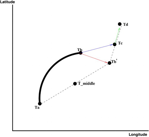
We consider that the glider acquires a GPS fix at time Ta, dives and then surfaces at time Tb. The thick line between Ta and Tb in Fig. A1 represents the extrapolated path using a dead reckoning algorithm. The glider “thinks” it surfaces at Tb but actually surfaces at Tb′, because of the current it experienced during the dive. The red arrow is then the depth-averaged current that affected the glider trajectory over the Ta-to-Tb time period.

The main issue is that the first GPS fix does not occur at Tb′ (i.e., exactly when the glider surfaces) but at a later time Tc. The deduced current is, therefore, the blue arrow in Fig. A1, which also includes the surface drift occurring between the time of surfacing (Tb′) and the first GPS fix (Tc).

To correct for this surface drift, the glider obtains a second GPS fix at a later time Td. It can, therefore, calculate the surface drift by dividing the difference in positioning at times Tc and Td by the time elapsed between Tc and Td (green arrow). The location of the glider at time Tb′ can be extrapolated by using this estimation of the surface drift and subtracting it from the glider’s position at time Tc. This technique provides a more accurate estimate of the depth-averaged current experienced by the glider during its last dive.

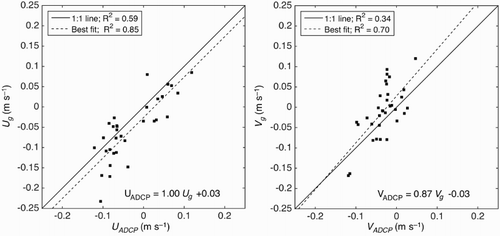
Each of these depth-averaged current estimations are then associated with the coordinates of the middle point of the glider’s dive (T_middle). All surfacings located within a 2 km radius from an ADCP mooring (T1, T2, or T3; Fig. 1b) are used to compare gliders’ current estimates to depth-averaged ADCP measurements. A linear fit is calculated and applied to all glider-based current estimate to calibrate the dataset with the ADCP observations ( Fig. A2).

Fig. A2 Comparison between the depth-averaged, cross-shore (U, left) and alongshore (V, right) currents measured by one of the ADCPs located at the T-station and the depth-averaged current experienced by the glider during a dive within a 2 km radius from an ADCP station. The goodness of fit R² between glider-based and ADCP observations is indicated for the non-calibrated datasets (1:1 line, solid line), as well as for the calibrated glider-based current using the linear equation indicated in the figures (best fit, dashed line).

Geostrophic currents are calculated using the thermal wind equation (Gill, 1982), based on the potential density indirectly measured by the glider. The data is gridded at a resolution of 1 km in the horizontal direction and 0.5 m in the vertical. The horizontal gradient in density is calculated using 2nd order finite differencing over 16 km, which corresponds to the internal Rossby radius of deformation in this region (Gill, 1982).

The velocity shear is then vertically integrated assuming a zero-velocity at the bottom. An offset is added to the geostrophic velocity so that the depth-averaged geostrophic velocity matches the across-path depth-averaged current deduced from glider drift. Plots of geostrophic currents superimposed with observations have been produced and demonstrate that this method yields very good comparisons (not shown).

Additional information

Funding

This research was supported by the Ocean Tracking Network (OTN), through a network project grant NETGP [grant number #375118-08] from the Natural Sciences and Engineering Research Council of Canada (NSERC) with additional support from the Canadian Foundation for Innovation (CFI) [grant number #13011], and the Social Sciences and Humanities Research Council (SSHRC) [grant number #871–2009-0001].