Dynamical Downscaling of the Arctic Climate with a Focus on Polar Cyclone Climatology

ABSTRACT

We present a dynamical downscaling of the Arctic climatology using a high-resolution implementation of the Polar Weather Research and Forecasting, version 3.6 (WRF3.6) model, with a focus on Arctic cyclone activity. The study period is 1979–2004 and the driving fields are data from the Hadley Centre Global Environmental Model, version 2, with an Earth System component (HadGEM2-ES) simulations. We show that the results from the Polar WRF model provide significantly improved simulations of the frequency, intensity, and size of cyclones compared with the HadGEM2-ES simulations. Polar WRF reproduces the intensity of winter cyclones found in ERA-Interim, the global atmospheric reanalysis produced by the European Centre for Medium-range Weather Forecasts (ECMWF), and suggests that the average minimum central pressure of the cyclones is about 10 hPa lower than that derived from HadGEM2-ES simulations. Although both models underestimate the frequency of summer Arctic cyclones, Polar WRF simulations suggest there are 10.5% more cyclones per month than do HadGEM2-ES results. Overall, the Polar WRF model captures more intense and smaller cyclones than are obtained in HadGEM2-ES results, in better agreement with the ERA-Interim reanalysis data. Our results also show that the improved simulations of Arctic synoptic weather systems contribute to better simulations of atmospheric surface fields. The Polar WRF model is better able to simulate both the spatial patterns and magnitudes of the ERA-Interim reanalysis data than HadGEM2-ES is; in particular, the latter overestimates the absorbed solar radiation in the Arctic basin by as much as 30 W m⁻² and underestimates longwave radiation by about 10 W m⁻² in summer. Our results suggest that the improved simulations of longwave and solar radiation are partly associated with a better simulation of cloud liquid water content in the Polar WRF model, which is linked to improvements in the simulation of cyclone frequency and intensity and the resulting transient eddy transports of heat and water vapour.

RÉSUMÉ

[Traduit par la rédaction] Nous présentons une réduction d’échelle dynamique de la climatologie arctique exécutée à l’aide d’une version à haute résolution du modèle Weather Research and Forecasting (WRF3.6) polaire, et étudions notamment l’activité cyclonique dans l’Arctique. La période d’étude s’étend de 1979 à 2004. Les données simulées de la version 2 du modèle environnemental mondial du Hadley Centre incluant le système terrestre, HadGEM2-ES, pilote le modèle. Nous montrons que les résultats du modèle WRF polaire améliorent grandement les simulations de la fréquence, de l’intensité et de la taille des cyclones par rapport aux simulations du HadGEM2-ES. Le modèle WRF polaire reproduit l’intensité des cyclones hivernaux présents dans les réanalyses atmosphériques mondiales ERA-Interim, que génère le Centre européen pour les prévisions météorologiques à moyen terme (CEPMMT). Il laisse penser que la pression centrale minimale des cyclones reste environ 10 hPa plus faible que celle émanant des simulations du HadGEM2-ES. Bien que les deux modèles sous-estiment la fréquence des cyclones estivaux de la région, les simulations du WRF polaire laissent croire qu’il se forme 10,5% plus de cyclones par mois que ne le montrent les résultats du HadGEM2-ES. Somme toute, le modèle WRF polaire résout plus de cyclones intenses et de petite taille que le HadGEM2-ES. Ses simulations correspondent davantage aux données de réanalyses ERA-Interim. Nos résultats montrent aussi que les simulations améliorées des systèmes synoptiques arctiques mènent à de meilleures simulations des champs atmosphériques en surface. Le modèle WRF polaire simule mieux les champs spatiaux et les magnitudes présents dans les réanalyses ERA-Interim que ne le fait le HadGEM2-ES. Notamment, ce dernier surestime parfois de 30 W m⁻² le rayonnement solaire absorbé dans le bassin arctique et sous-estime d’environ 10 W m⁻² le rayonnement d’ondes longues en été. Nos résultats semblent indiquer que les simulations améliorées des rayonnements solaire et d’ondes longues proviennent partiellement d’une meilleure simulation du contenu en eau liquide des nuages dans le modèle WRF polaire. Cette bonification entraîne aussi l’amélioration de la fréquence et de l’intensité simulées, ainsi que du transport par tourbillon transitoire de chaleur et de vapeur d’eau qui en découle.

KEYWORDS:

• Arctic cyclone climatology
• dynamical downscaling
• Polar WRF
• surface radiation

1 Introduction

It has been recognized that global climate models (GCMs) are useful tools for understanding potential climate change on the scale of ocean basins. However, they lack the spatial resolution to resolve fine-resolution details, such as the complicated coastlines and narrow straits of the Canadian Arctic Archipelago. By comparison, a regional climate model can be run at a high resolution and relatively low cost and thus constitutes a useful alternative to GCMs. In order to provide high-resolution surface fields to study climate change in the Arctic Ocean, we used a dynamical regional downscaling system based on the Polar Weather Research and Forecasting (Polar WRF) model to downscale coarse-resolution GCM estimates. The GCM used is the Hadley Centre Global Environmental Model, version 2, with an Earth System component (HadGEM2-ES) with a resolution of 1.25° × 1.875° in latitude and longitude. The Polar WRF was implemented on a 25 km resolution regional atmospheric grid. One of the objectives of this study is to evaluate the accuracy of downscaled simulations for the present-day climate relative to reanalysis data for the period 1979–2004. In a later study, we will construct high-resolution, regional climate change projections of the atmospheric forcing over the Arctic, following scenarios from the Intergovernmental Panel on Climate Change.

A finer resolution regional model can potentially better represent small-scale surface processes related to topography and other surface heterogeneities (Blender & Schubert, 2000; Giorgi & Mearns, 1991). Several studies have shown that finer resolution regional models resolve small-scale fields, such as extratropical cyclones, more accurately than coarse-resolution GCMs (e.g., Denis, Laprise, & Caya, 2003; Guo et al., 2013; Long, Perrie, Gyakum, Laprise, & Caya, 2009). Coarse-resolution GCMs tend to underestimate the number and intensity of these small-scale systems, primarily because of dissipation of the kinetic energy of mesoscale motions (Blender & Shubert 2000; Jung, Gulev, Rudeva, & Soloviov, 2006) resulting from the associated over-smoothed spatial structures of the baroclinic Rossby waves (Béguin et al., 2013), as well as the low spatial scale resolution of the reanalysis data (Condron, Bigg, & Renfrew, 2006). In particular, Nishii, Nakamura, and Orsolini (2015) documented that even with the improvements in the Coupled Model Intercomparison Project, phase 5 (CMIP5) models compared with CMIP, phase 3 (CMIP3) models, most climate models still underestimate summer Arctic storm tracks.

It has been recognized that Arctic cyclones are crucial in the Arctic climate. The atmospheric surface fields, including sea level pressure (SLP), surface wind, and surface radiation, represent the cumulative effects of synoptic weather systems. Arctic cyclone activity plays a key role in air–sea interactions and is a potential factor in Arctic warming and unprecedented sea-ice decline over the last few decades (Screen, Simmonds, & Keay, 2011; Simmonds, 2015; Stroeve, Holland, Meier, Scambos, & Serreze, 2007; Zhang, Walsh, Zhang, Bhatt, & Ikeda, 2004). Some studies report a direct influence of intense cyclones on the sea-ice cover on synoptic time scales (Parkinson & Comiso, 2013; Ono, Inoue, Yamazaki, Dethloff, & Yamaguchi, 2016; Simmonds & Keay, 2009; Zhang, Lindsay, Schweiger, & Steele, 2013; Zhang, Lindsay, Steele, & Schweiger, 2008). Moreover, changes in Arctic cyclones largely reflect changes in the atmospheric circulation (Ledrew, 1984, 1988; Serreze & Barrett, 2008), which can potentially result from an amplification of the Arctic warming and a decline in Arctic sea ice (e.g., Cavallo & Hakim, 2013; Screen, Simmonds, Deser, & Tomas, 2013, 2014). Arctic cyclones play a central role in high-latitude atmospheric heat and moisture transports from mid-latitudes that can change cloud feedbacks affecting the retreat of sea ice (Screen et al., 2011). Underestimates of cyclone numbers and intensity can lead to deficiencies in the estimates for the poleward energy transport into the Arctic and can also affect surface heat fluxes and radiation associated with clouds. Nevertheless, when the resolution is increased sufficiently, regional model results can achieve improved simulation of cyclone activity compared with reanalysis results (i.e., Shkolnik & Efimov, 2013; Wang et al., 2004), capturing the more frequent and more intense Arctic cyclones (Tilinina, Gulev, & Bromwich, 2014). Therefore, in this study we focus on the simulation of Arctic cyclone activity to validate and evaluate dynamic downscaling using the Polar WRF regional model.

In addition, it has been argued that Arctic cyclones show differences in their structure and behaviour compared with mid-latitude cyclones (e.g., Reed, 1979; Simmonds & Rudeva, 2014; Tanaka, Yamagami, & Takahashi, 2012) because of the unique characteristics of the Arctic atmosphere (Reed, 1979). These characteristics include generally small cyclone sizes (Reed, 1979) and dynamic processes associated with polar vortices in the Arctic tropopause (Simmonds & Rudeva, 2014; Tanaka et al., 2012; Yamazaki, Inoue, Dethloff, Maturilli, & König-Langlo, 2015). The upper level circulation polar vortex in the Arctic is very important for surface cyclogenesis and development (e.g., Cavallo & Hakim, 2012; Long & Perrie, 2012; Serreze, 1995; Serreze & Barry, 2005; Simmonds & Rudeva, 2012, 2014; Tanaka et al., 2012; Yamazaki et al., 2015). Numerical experiments by Yamazaki et al. (2015) have suggested that improved reproduction of upper tropospheric circulation in the Arctic region is indispensable for realistic simulation of Arctic cyclones because of the essential role of the polar vortex in the baroclinic instability of the Arctic atmosphere. This is another reason to evaluate the dynamic downscaling simulation of Arctic cyclones.

Our study presents an analysis of cyclone statistics simulated by the Polar WRF model, implemented in the Arctic at a spatial resolution of 25 km, driven by a HadGEM2-ES simulation. The motivation of the paper is to evaluate the ability of the Polar WRF model to simulate Arctic cyclones and related surface fields, such as SLP, surface wind, and surface radiation, by comparing the results with GCM results. Cyclones are identified by application of the advanced cyclone track detection scheme developed at the University of Melbourne (Murray & Simmonds, 1991, 1995). Thus, in this study we evaluate the dynamical downscaling of the Arctic climate with the regional Polar WRF model. Our perspective is different from previous studies in that we investigate not only the better performance of our approach in the simulation of cyclone activity but also the associated improvements in the simulation of atmospheric surface fields, SLP, and surface radiation. Thus, we demonstrate the potential importance of this approach to dynamical downscaling in simulations of the present Arctic climate.

The paper is organized as follows. Section 2 briefly describes the Polar WRF model, the experimental design, the data used in this study, and the analysis methods. Section 3 demonstrates the improved simulations of Arctic cyclone climatology in both cold and warm seasons compared with the estimates from HadGEM2-ES and the reanalysis data. Section 4 discusses the improved surface fields that result from better Arctic cyclone simulations. Section 5 provides a discussion and summary.

2 Models and reanalysis data

a Polar WRF

The Polar WRF model used in this study is based on the polar-optimized WRF, version 3.6 (i.e., Hines et al., 2015). The polar optimizations used in the Polar WRF model (Bromwich, Hines, & Bai, 2009; Hines & Bromwich, 2008; Hines, Bromwich, Bai, Bitz et al., 2015; Hines, Bromwich, Bai, Barlage, & Slater, 2011) focus on improvements to the Noah land scheme model, including the use of fractional sea ice within each grid cell and the specification of a number of sea-ice characteristics including thickness, snow cover on sea ice, and albedo. Changes to heat transfer and a revised surface-energy balance calculation have also improved the performance of Polar WRF over all snow and ice surfaces.

The choice of physical parameterizations for the simulations described here is based upon previous Polar WRF applications (e.g., Bromwich et al., 2009; Hines et al., 2011). Subgrid-scale cumulus is parameterized with the Grell and Dévényi (2002) ensemble scheme, and the two-moment Morrison scheme (Morrison, Curry, & Khvorostyanov, 2005) is applied for cloud microphysics. Lower atmospheric and surface physics include the use of the Mellor–Yamada–Janjić (MYJ) planetary boundary layer scheme in conjunction with the eta surface layer scheme based on similarity theory (Janjić, 1994). Radiation schemes include the Rapid Radiative Transfer Model for longwave radiation and the Goddard scheme for shortwave radiation.

In our simulations, the model was initialized on 1 January 1969 and integrated to 31 December 2004. The model domain is shown in Fig. 1e as a blue box, in which the shading represents the sea-ice concentration prescribed in the Polar WRF model. The horizontal resolution is 25 km (Table 1), with 38 terrain-following sigma levels to 20 hPa. Daily sea-ice concentration, sea-ice thickness, sea surface temperature, monthly sea-ice albedo, and snow depth on the sea ice were specified for each ocean grid point in the model domain. The initial and lateral boundary conditions for Polar WRF were provided by 6-hourly outputs from HadGEM2-ES simulations. Before the validation of the Polar WRF simulations, we compared the climatological mean of the prescribed sea-ice concentration in the Polar WRF from the HadGEM2-ES (Figs 1e–1h) with observations (Figs 1a–1d) from the Hadley Centre Sea Ice and Sea Surface Temperature (HadISST) dataset (Rayner et al., 2003). It is important to make this comparison initially because the Arctic atmosphere is very sensitive to the surface boundary conditions, especially sea-ice cover. The comparison shows that the spatial distributions of prescribed sea-ice concentrations compare reasonably well with HadISST data although the summer and autumn sea-ice concentrations are underestimated.

Fig. 1 (a) to (d) Four seasons mean sea-ice concentration (shading) from the observed HadISST data; (e) to (h) as in (a) to (d) but from the HadGEM2-ES to be prescribed in the Polar WRF simulation. The blue boxes in (e) to (h) indicate the model domain used in the simulation of Polar WRF.

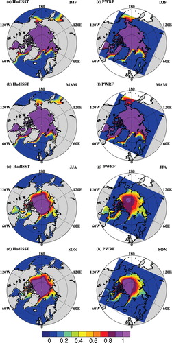
Table 1. Detailed information for the two models, Polar WRF 3.6 and GCM HadGEM-ES2, as well as the ERA-Interim reanalysis dataset.

Models	Spatial Resolution	Temporal Resolution	Validation Time Period
ERA-Interim (ERAI)	T255 (0.75° × 0.75°)	6-hours (SLP), monthly mean	1979–2004
HadGEM-ES2	Atmosphere: N96, (1.25° × 1.875°) Ocean: 1° × 1°	6-hours (SLP), monthly mean	1979–2004
Polar WRF	25 km × 25 km	6-hours (SLP), monthly mean	1979–2004

The simulation presented in this study is not nudged toward the large-scale driving data from HadGEM2-ES. We also conducted a second simulation (not presented) with the same implementation but with spectral nudging of the middle and upper level tropospheric wind and temperature (Glisan, Gutowski, Cassano, & Higgins, 2013). There are small differences in the magnitudes between these two simulations for the circulations and surface fields that we present in this study, and, based on the Student’s t-test, these differences are insignificant at the 95% confidence level.

b HadGEM2-ES

In our study, Polar WRF was driven by the data (1969–2004) generated by a global climate earth system model, namely, HadGEM2-ES. In a follow-on paper, we continue the simulation using the Representative Concentration Pathway, version 8.5 (RCP 8.5) climate change scenario for 2005 to 2100. As documented in detail by Collins et al. (2011), HadGEM2-ES includes a coupled atmosphere–ocean global climate model (AOGCM) with appropriate additional schemes for related processes of the Earth climate system. The atmospheric component uses a horizontal resolution of 1.25° × 1.875° in latitude and longitude (“N96”) (Table 1) with 38 layers in the vertical extending to more than 39 km in altitude. The oceanic component uses a latitude–longitude grid with a zonal resolution of 1° and a meridional resolution of 1° between the poles and 30° latitude and increases smoothly to 1/3° at the equator. It has 40 unevenly spaced levels in the vertical. Although the physical basis of the processes represented within HadGEM2-ES has been updated with adjusted physical parameterizations that are suitable for the relatively high resolution of this implementation, these physical schemes are still relatively simple and usually use first-order approximations (Martin et al., 2006). For example, the convection scheme for cumulus convection is diagnosed using the mean humidity profile, and the radiative effects of convective anvils are represented by specifying the vertically varying convective cloud amount (Gregory & Rowntree, 1990). Moreover, for the cloud scheme, the cloud water and cloud amount are diagnosed from total moisture and liquid water potential temperature using a triangular probability distribution function (Smith, Gregory, Wilson, Bushell, & Cusack, 1999). The boundary layer scheme is a first-order turbulence closure mixing scheme with adiabatically conserved variables (Lock, Brown, Bush, Martin, & Smith, 2000).

c Reanalysis Data

Six-hourly global mean sea level pressure (MSLP) and monthly circulation fields from ECMWF reanalysis products ERA-Interim (Dee et al., 2011) are used to validate Polar WRF simulations. ERA-Interim is one of the most modern reanalyses, employing new physics parameterizations, a 12 h four-dimensional variational data assimilation (4DVAR) system, and variational bias correction of the observed radiances (Simmons, Uppala, Dee, & Kobayashi, 2007). ERA-Interim output is available at T255 horizontal resolution (0.75° × 0.75°; Table 1), with 60 hybrid layers in the vertical. Previous studies (e.g., Porter, Cassano, & Serreze, 2011) have demonstrated that ERA-Interim is reliable, based on comparisons of the radiation budget in the Arctic to data from field experiments, such as the Surface Heat and Energy Budget of the Arctic (SHEBA) experiment and Clouds and the Earth’s Radiant Energy System (CERES) observations.

d Cyclone Tracking Algorithm

Arctic cyclones are detected and tracked by applying the cyclone identification algorithm developed at the University of Melbourne (Murray & Simmonds, 1991, 1995; Pezza, Simmonds, & Renwick, 2007) to the SLP fields. The cyclone tracking scheme has been shown to perform well in a number of comparisons (e.g., Raible, Della-Marta, Schwierz, Wernli, & Blender, 2008; Uotila, Pezza, Cassano, Keay, & Lynch, 2009). This scheme has a reasonably high level of sophistication in that, rather than the Eularian perspective of cyclone behaviour, it uses the quasi-Lagrangian perspective which has been seen as more appropriate, especially in the Arctic basin. Concisely described, the algorithm objectively identifies cyclones at 6-hourly intervals based on the structure of the MSLP fields, by comparing the Laplacian of pressure (LP), ∇² p at each grid point with those at neighbouring grid points and identifies both open and closed low pressure systems. We ignore MSLP cyclones at locations where the surface elevation exceeds 1 km because MSLP has little dynamic meaning in those circumstances.

The tracking scheme produces fields of cyclone frequencies and properties. The cyclone properties calculated by the scheme include the system density, rates of cyclogenesis (FG) and cyclolysis (FL), the mean central pressure of cyclones, the mean system intensity (CC), the mean cyclone radius (R) over a unit area, and the track number. The definition of these variables has been described in the literature (Simmonds, Burke, & Keay, 2008). The precise value calculated for the cyclone frequencies depends on the choice of input parameters associated with the spatial resolutions of the SLP. Uotila et al. (2009) applied this algorithm to multiple datasets with different resolutions and ran sensitivity experiments for 165 different input parameter combinations to determine the most appropriate values for each. Given the similarity in resolution of the datasets used here (ERA-Interim) and the Antarctic Mesoscale Prediction System (AMPS; 60 (90) km resolution at the end (beginning) of their study period), their parameter values (listed in Table 1 of Uotila et al., 2009) were also considered appropriate for our current study.

Tracking cyclones in a limited domain includes the so-called entry-exit uncertainties resulting from the presence of cyclones generated, or decaying, outside (or inside) the domain. To avoid the impact of these cyclones on the tracking results, we consider only cyclone tracks entering the 70°N latitude circle, which is the polar cap domain. Also, we eliminated any tracking outputs with a lifetime less than 12 hours.

In this study, we only discuss two major Arctic cyclones in two seasons, one in the cold and frozen season and the other in the warm, ice-melting season. Therefore, we define the cold season as the period from November to March and the warm season as the period from June to October. However, in Section 4, when discussing the atmospheric surface fields, we will follow the conventional definition of winter (December–February), spring (March–May), summer (June–July), and autumn (September–November).

3 Arctic cyclone climatology

a Cold Season Cyclones

The majority of Arctic cyclones in the cold months (November–March; Fig. 2a) move into the Arctic Ocean from the North Atlantic as a result of the southwestern steering flow of the eastern North American trough (e.g., Serreze & Barry, 2005). The overall pattern in Fig. 2a is similar to the results shown in previous studies using the same tracking scheme (Simmonds et al., 2008) or other methodologies (e.g., Serreze & Barry, 2005). There are two main cyclone tracks into the Arctic basin from the North Atlantic. One enters the Arctic Ocean through the East Greenland Sea and the other moves eastward into the Barents Sea, as suggested by the two maxima near the East Greenland Sea and Barents Sea. The cyclones in the North Pacific, associated with the Aleutian Low, are typically blocked from entering the Arctic by a ridge extending from eastern Siberia to northwestern North America (Serreze & Barry, 2005). Cyclones that form over the Eurasian continent tend to migrate southeastward as a result of the northwest steering flows of the eastern Asian trough, resulting in relatively few cyclones in the Beaufort and Chukchi Seas (Serreze & Barry, 2005).

Fig. 2 Shading indicates cyclone track density (mean number of cyclone tracks per unit per month) in the cold season (November–March) for the period 1979–2004 for the region north of 66°N derived from (a) ERA-Interim reanalysis data; (b) the difference between HadGEM2-ES and the ERA-Interim reanalysis data and (c) Polar WRF and the ERA-Interim reanalysis data, respectively. Corresponding densities of cyclogenesis are given in (d), (e), and (f) as in (a), (b), and (c), respectively (the mean number of genesis events in a 10³ (°latitude)² area per month).

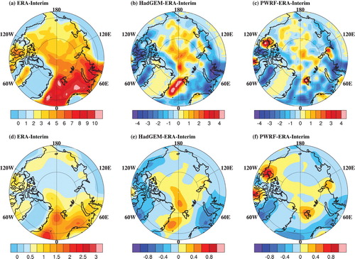
Track density estimates simulated by HadGEM-ES2 and Polar WRF are shown in Figs 2b and 2c. Results from both HadGEM-ES2 and Polar WRF capture the overall spatial patterns in the ERA-Interim data (Fig. 2a). For example, there are two main tracks of cyclones on the Atlantic side of the Arctic. Compared with the ERA-Interim and Polar WRF simulations, HadGEM-ES2 significantly overestimates the cyclone tracks in the East Greenland Sea and underestimates the cyclone tracks in the Barents and Kara Seas. By comparison, Polar WRF gives a more reasonable simulation in the East Greenland Sea although results are underestimated in the Barents and Kara Seas. The bias in HadGEM2-ES simulations for cyclone tracks is partly due to the bias in the cyclogenesis (Fig. 2e) and the westward displaced steering flow, which results from a slight westward displacement of the Ural trough in comparison with that in ERA-Interim or Polar WRF (figure not shown). Similar to the cyclone tracks (Fig. 2c), the cyclogenesis is captured well in Polar WRF simulations but slightly underestimated in the Barents and Kara Seas (Fig. 2f). Over the Beaufort Sea, the track densities are overestimated by Polar WRF and underestimated by HadGEM2-ES, as shown in the cyclogenesis plots.

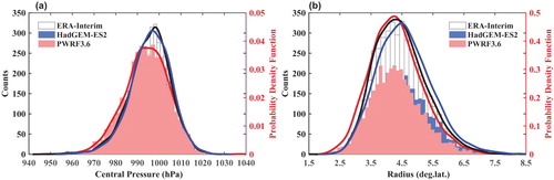
On average, the cyclones in HadGEM2-ES simulations are much weaker than in the ERA-Interim data or the Polar WRF simulations, as shown in the central pressure histograms in Fig. 3a. Specifically, there are more weak cyclones in the HadGEM2-ES simulations, with a minimum central pressure of at least 1000 hPa, than in the ERA-Interim dataset and Polar WRF simulations. Although cyclone frequency is slightly underestimated in the Polar WRF simulations compared with ERA-Interim results, the cyclone intensity distribution simulated by Polar WRF is consistent with that in ERA-Interim. Figure 3a also shows the estimated probability distribution functions (PDFs) of minimum cyclone central pressure, using a nonparametric fit to all 135 cold months from the ERA-Interim reanalysis data (black curve), as well as results from Polar WRF (red curve) and HadGEM2-ES simulations (blue curve). The resulting PDFs for cyclone frequencies, for ERA-Interim and Polar WRF are identical at the 99% confidence level, based on the Kolmogorov-Smirnov test (Massey, 1951), with mean values of 995 hPa. However, the PDF mean value associated with HadGEM2-ES simulations (blue curve) is statistically different from the ERA-Interim results (black curve) at the 99% confidence level by about 10 hPa. On average, in the cold Arctic winter months, Polar WRF suggests a total of 27.9 cyclone tracks for each month, which is similar to the HadGEM2-ES simulations with a monthly mean of 28.0 cyclone tracks. Moreover, both models simulate 13.2% fewer cyclone tracks in the polar cap region than suggested by ERA-Interim data, which has a monthly average of 32.2 cyclone tracks.

Fig. 3 Climatological occurrence histograms of (a) minimum cyclone central pressure and (b) radius in individual cyclone tracks over the polar cap (north of 70°N) during winter (November–March) for the period 1979–2004. The pink bars represent cyclone tracks from the Polar WRF model, while the blue and white bars show the results from HadGEM2-ES and the ERA-Interim reanalysis, respectively. The solid black curve illustrates the probability distribution function (PDF) of (a) minimum cyclone central pressure and (b) radius, based on all 135 winter months from the ERA-Interim reanalysis. The red and blue curves show the results from the Polar WRF model and the HadGEM2-ES simulations. Nonparametric PDFs are constructed using MATLAB, utilizing kernel density estimation.

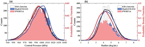
In terms of size, although most cold winter cyclones have radii between 3° and 5° latitude, Polar WRF cyclones are smaller (radius <3.2° latitude) than those of either ERA-Interim or HadGEM2-ES (bars in Fig. 3b). Moreover, Polar WRF simulates fewer large cyclones (radius >4.8° latitude) than HadGEM2-ES. This is apparent from a visual comparison of the three PDFs based on the sizes of cyclones in each of the three datasets during the cold months. The three PDFs have similar mean values, around 4.2°–4.5° latitude, but the PDF for Polar WRF has a shift toward smaller cyclones, indicating a higher possibility of these occurrences compared with ERA-Interim data or the HadGEM2-ES simulations.

b Warm Season Cyclones

The patterns of Arctic cyclones in the warm season (June–October; Fig. 4a) are very different from the wintertime cold season patterns (Fig. 2a). Cyclone activity in the Norwegian and Barents Seas is much less prominent. Cyclones occur most frequently over the central Arctic Ocean, primarily because of the migration of synoptic systems generated over Eurasia and along the dominant (but weakened) North Atlantic cyclone track (e.g., Serreze & Barry, 2005; Serreze, Barry, Rehder, Walsh, & Drewry, 1995). These cyclones tend to be generated either over northern Eurasia or along the Eurasian coast, where there is a strong temperature contrast in the warm months. Winds at 500 hPa tend to steer storms parallel to the coast across Eurasia and Alaska. The cyclones that enter, or are formed within, the Arctic almost invariably decay within, or in close proximity to, the Arctic basin, especially in the central Arctic. Thus, there is a cyclone maximum over the central Arctic Ocean, which is a prominent feature documented in previous studies (Serreze & Barrett, 2008; Simmonds & Rudeva, 2012; Yamazaki et al., 2015). Both models (Figs 4b and 4c) capture the overall spatial patterns well when compared with the ERA-Interim data, but both underestimate the number of warm season cyclones. Polar WRF simulates a considerably higher number of cyclones in the whole Arctic basin than HadGEM2-ES but still fewer than are estimated by the ERA-Interim data. Overall, HadGEM2-ES underestimates the number of cyclones more seriously, especially in the central Arctic. These significant deficiencies in simulations of warm season cyclones have a crucial effect on associated estimates for the surface-energy budget, through the cloud radiative effect, which will be demonstrated in Section 4.b.

Fig. 4 Cyclone track density (mean number of cyclone tracks per unit per month) in the warm season (June–October) over the period 1979–2004 for the region north of 70°N derived from (a) the ERA-Interim reanalysis; (b) and (c) show the difference between HadGEM2-ES and the ERA-Interim reanalysis data and Polar WRF and the ERA-Interim reanalysis data, respectively. Densities of cyclogenesis (the mean number of genesis events in a 10³ (°latitude)² area per month) are given in (d), (e), and (f), corresponding to (a), (b), and (c), respectively. Densities of cyclolysis are given in (g), (h), and (i), corresponding to (a), (b), and (c), respectively.

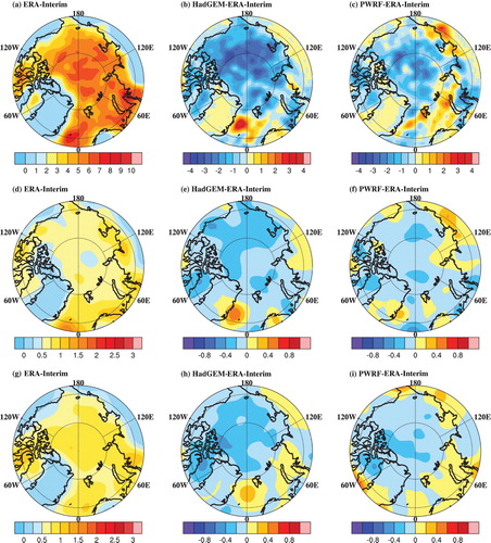
In the HadGEM2-ES simulations, the underestimates in cyclone track density are partially due to the lower rates of cyclogenesis (Fig. 4e) and fewer cyclolysis events (Fig. 4h). Evidently, Polar WRF agrees better with the ERA-Interim data than does HadGEM2-ES. Both models (Figs 4e and 4f) reproduce the regions of the largest cyclogenesis events in the open water areas over the Atlantic side of the Arctic and the coastal area extending across Eurasia and Alaska compared with the ERA-Interim reanalysis data (Fig. 4d). Compared with Polar WRF, HadGEM2-ES has a greater tendency to underestimate cyclogenesis events over the central Arctic, as well as over the coastal regions of the East Siberian Sea, the Chukchi Sea, and the Beaufort Sea. However, both models (Figs 4h and 4i) capture the spatial patterns of cyclolysis events well, although HadGEM2-ES greatly underestimates the cyclolysis events in the central Arctic region because of fewer cyclogenesis activities in the Arctic; thus, fewer cyclones are available to die in the central Arctic. Although Polar WRF results also slightly underestimate cyclolysis events in the area near the North Pole, its simulations compare more favourably with ERA-Interim data than those of HadGEM2-ES, especially in North Eurasian coastal areas. It is noted that both the GCM HadGEM-ES2 and Polar WRF simulate cold season cyclones better than warm season ones; this result may relate to the more complicated surface processes involved with increasing solar radiation and open water areas in the warm season.

Key features of the cyclone frequency distributions in the warm season, including intensity and size, are presented in Fig. 5. These results are similar to those found for cold season cyclones in Fig. 3. Compared with HadGEM2-ES results, Polar WRF captures significantly more intense cyclones with smaller sizes in the warm months. Compared with ERA-Interim data (white bars in Fig. 5a), results from Polar WRF (red bars in Fig. 5a) also capture a higher number of intense cyclones with central pressures less than 990 hPa. This is achieved even though in the Polar WRF results the total number of cyclone tracks, on average 28.4 per warm season month, is 11.5% less than that derived from the ERA-Interim data, which has an average of 32 cyclone tracks per month. Moreover, the HadGEM2-ES simulations, with a total of 25.7 cyclone tracks per month, underestimate the number of cyclone tracks over the polar cap region by about 19.9% compared with ERA-Interim data. The results from HadGEM2-ES also suggest fewer cyclones with lower central pressures (more intense) although comparable numbers of cyclone tracks with relatively high central pressures (>1005 hPa) are captured. In total, Polar WRF captures 10.5% more cyclone tracks than HadGEM2-ES in the warm season.

Fig. 5 As in Figs 3a and 3b but for the Arctic warm months (June–October).

Comparing the areas under the curves, there is a higher probability of cyclone track occurrences with lower minimum central pressures in the Polar WRF (red curve) results than in the ERA-Interim reanalysis data (black curve) or in the HadGEM2-ES simulations (blue curve). The two PDFs for results from ERA-Interim and HadGEM2-ES are very close, with the same mean value of about 1000 hPa. By comparison, the results from the PDF for Polar WRF exhibit a broad mean value, in the range of 990–998 hPa, which is shifted toward more intense cyclones. In terms of cyclone sizes, the distributions of cyclone radii (Fig. 5b) basically show that the number of cyclones in the ERA-Interim data (white bars) exceeds the cyclone numbers suggested by the two models over the entire range of the cyclone radii, whereas Polar WRF results (pink bars) suggest smaller sizes and fewer large cyclones than the HadGEM2-ES simulations (blue bars). Also, note that the mean size of Arctic cyclones is smaller than that of mid-latitude cyclones as suggested by Simmonds (2000), consistent with previous studies (e.g., Reed, 1979). It is clear from a visual inspection of Fig. 5b, regarding the estimated PDFs for the size of cyclones (with respect to minimum central pressure for individual tracks), that the Polar WRF data (red curve) exhibit a shift toward smaller cyclone radii compared with HadGEM2-ES data (blue curve). These results reflect the finer horizontal resolution used by Polar WRF.

4 Atmospheric surface fields in the Arctic

a Sea Level Pressure and Surface Wind

The seasonal mean SLP fields from Polar WRF and HadGEM-ES2 model simulations, averaged over the 26-year period of this study, are compared with ERA-Interim data, as shown in Fig. 6. The overall positions, magnitudes, and seasonal cycles of the major systems, including the Icelandic Low, Aleutian Low, and the Beaufort High shown in ERA-Interim data (left panel in Fig. 6), are well reproduced by both models. In summer (Figs 6g and 6i), the Siberian High is replaced by a thermal low; the Beaufort High is weak, and the Aleutian and Icelandic Lows nearly disappear, partly because the frequency of cyclones in the northern oceans decreases considerably. Meanwhile, there is a weak low centred almost directly under the core of the 500 hPa polar vortex over the North Pole, which corresponds to the summer cyclone maximum centre (Fig. 4a) over that region (Serreze & Barrett, 2008).

Fig. 6 Mean sea level pressure (SLP; shading; hPa) and surface wind (vectors; m s⁻¹) for four seasons (a), (d), (g), and (j) from ERA-Interim reanalysis data; (b), (e), (h), and (k) show the difference between HadGEM2-ES and the ERA-Interim reanalysis data; (c), (f), (i), and (l) show the difference between Polar WRF and the ERA-Interim reanalysis data, respectively.

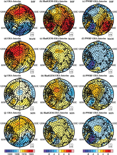
Compared with the ERA-Interim reanalysis data, the results from HadGEM-ES2 overestimate the strength of the Beaufort High in all seasons (Fig. 6, middle column) and underestimate the weak summer low over the central Arctic (Fig. 6h). The bias in the intensity of the Beaufort High is associated with fewer, weaker cyclones in the Beaufort Sea (Figs 2b and 4b). Underestimates of the weak summer low are due to greatly underestimated cyclone densities in the central Arctic (Fig. 4b). By contrast, Polar WRF results simulate the Beaufort High reasonably well (Fig. 6, right panels) although they also slightly underestimate the weak summer low (Fig. 6i). Likewise, improvements in the simulations of the Beaufort High and summer low from Polar WRF are consistent with reliable simulations of synoptic cyclones suggested by this model.

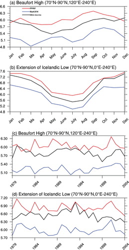
Figure 7 shows the annual cycles of surface wind speeds at 10 m averaged over the regions of the Beaufort Sea High (70°–90°N, 120°–240°E; Fig. 7a) and the extension of the Icelandic Low in the Barents and Kara Seas (70°–90°N, 0°–120°E; Fig. 7b). These results suggest that Polar WRF simulates the strongest surface winds in all seasons, whereas HadGEM-ES2 produces the weakest surface winds and ERA-Interim reanalysis data give relatively moderate-to-intermediate results. The time series of interannual variations in surface wind speeds over the validation period (1979–2004) show similar and consistent biases over these annual cycles (Figs 7c and 7d). The remarkable differences between results from HadGEM-ES2, Polar WRF, and ERA-Interim can be partially attributed to the higher number of more intense, smaller cyclones that are systemically found in the results from Polar WRF and in ERA-Interim data, compared with those of HadGEM-ES2 (Figs 2–5).

Fig. 7 Annual cycles of surface wind speed at 10 m height (m s⁻¹) for the period 1979–2004 derived from ERA-Interim reanalysis data (black line), HadGEM2-ES data (blue line), and our Polar WRF results (red line), averaged over the region of (a) the Beaufort High (70°–90°N, 120°–240°E and (b) the extension of the Icelandic Low in the Barents and Kara Seas (70°–90°N, 0°–120°E; (c) and (d) as in (a) and (b) but for the annual mean variations of surface wind speed at 10 m height.

b Surface downward radiation

1 surface radiation

Figure 8 shows the annual cycle of the net longwave (LW_SFC), shortwave (SW_SFC) radiation at the surface, and the sum of the net longwave and shortwave radiation, which is the net radiation at the surface (R_SFC) for the north polar cap region. Here, all radiative fluxes are positive upward. Monthly mean SW_SFC is negative during the summer when R_SFC is at its peak (Fig. 8a). Compared with the ERA-Interim data (black curves), the results from Polar WRF (red curves) reproduce the annual cycle of SW_SFC quite well, whereas results from HadGEM-ES2 overestimate the absorbed (negative in our convention) shortwave radiation by as much as 20 W m⁻² in summer (June to August). The SW_SFC bias in HadGEM-ES2 data is present for most months when at least a portion of the polar cap region is sunlit. The LW_SFC results for HadGEM-ES2 are slightly larger than those found in the results from Polar WRF or ERA-Interim data over the entire year. In results from the two models and the ERA-Interim results, the annual cycles of R_SFC follow the same patterns as those of SW_SFC although they are modulated by the LW_SFC contributions. Compared with ERA-Interim reanalysis data, results from HadGEM-ES2 overestimate the net surface radiation R_SFC by as much as 20 W m⁻² in summer. By contrast, results from Polar WRF suggest 69.6 W m⁻² as the summer mean, which compares well with the estimate of 70.9 W m⁻² from the ERA-Interim data.

Fig. 8 (a) Annual cycle of surface net radiation (solid lines) and its shortwave (SW, dashed lines) and longwave (LW, dotted lines) radiative components averaged over the polar cap. The explicit subscript “SFC” has been omitted. Black lines are based on the ERA-Interim reanalysis data; blue and red lines indicate results from HadGEM2-ES and Polar WRF data, respectively. All fluxes are positive upward (W m⁻²); (b) as in (a) but for surface downward radiation.

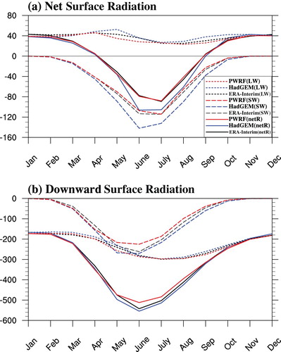
The differences between the SW_SFC results for the two models are mainly related to the differences in the downward shortwave radiation (SWD_SFC; Fig. 8b) because the sea-ice fraction and albedo are prescribed in Polar WRF simulations, as in the HadGEM2-ES simulations. As shown in Fig. 8a, results from Polar WRF suggest that the summer SWD_SFC is underestimated for the Arctic basin (red dashed curve in Fig. 8b), whereas the summer SWD_SFC is overestimated by HadGEM-ES2 simulations (blue dashed curve in Fig. 8b). Moreover, differences in the LW_SFC results can largely be attributed to the differences in the downward longwave radiation (LWD_SFC), given the consistent values for outgoing surface longwave radiation because of similar surface temperatures in both models (figure not shown). The LWD_SFC is underestimated by HadGEM-ES2 (blue dotted curve in Fig. 8b) and is slightly overestimated by Polar WRF (red dotted curve in Fig. 8b), as shown in the net LW_SFC values (dotted curves in Fig. 8a). Although Polar WRF underestimates the SWD_SFC (red dashed curve in Fig. 8b), the net SW_SFC values agree well with the ERA-Interim data (dashed curves in Fig. 8a), suggesting smaller surface albedo in results from Polar WRF.

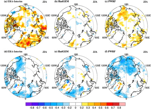
Regarding the spatial patterns of SW_SFC, the HadGEM-ES2 simulations (Fig. 9b) overestimate the net SW_SFC over the sea ice by as much as 40 W m⁻² (Fig. 9j) compared with ERA-Interim data (Fig. 9a), whereas the Polar WRF results (Fig. 9c) capture the spatial patterns of the absorbed SW_SFC, with overestimates of about 10 W m⁻² near the North Pole and underestimates on the Atlantic side of the Arctic of about 40 W m⁻² (Fig. 9k). In both the Polar WRF simulation and the ERA-Interim data, the SW_SFC values exhibit primarily zonal patterns in the Arctic basin with a maximum over the central Arctic. By comparison, the maximum SW_SFC in the HadGEM-ES2 results (Fig. 9b) is located in the western Arctic Ocean. Therefore, it is clear that the absorbed SW_SFC, as simulated in the Polar WRF results, agrees more closely with the ERA-Interim data than with the HadGEM-ES2 results, particularly in the Arctic basin.

Fig. 9 Climatological mean surface net shortwave (SW) radiation for summer (June–August; JJA) during the current climate from 1979 to 2005 for (a) ERA-Interim, (b) HadGEM2-ES, and (c) Polar WRF. All fluxes are positive upward; (d), (e), and (f) as in (a) to (c), but for downward shortwave radiation at the surface; (g) to (i) as in (a) to (c) but for downward longwave radiation at the surface. Difference between (j) surface net shortwave (SW) radiation from HadGEM2-ES and the ERA-Interim reanalysis data and (k) surface net shortwave (SW) radiation from Polar WRF and the ERA-Interim reanalysis data; (l) and (m) as in (j) and (k) but for downward shortwave radiation at the surface; (n) and (o) as in (j) and (k) but for downward longwave radiation at surface.

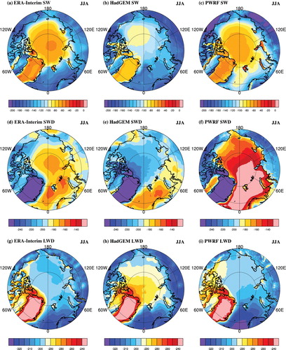
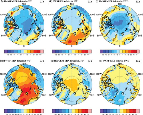
The differences in net SW_SFC are the result of the differences in the downward shortwave components of SWD_SFC (Figs 9d–9f). Compared with the ERA-Interim data (Fig. 9d), HadGEM-ES2 (Fig. 9e) simulates unrealistic distributions of downward shortwave radiation over the Arctic basin, and its maximum shifts toward the Canadian Arctic Archipelago. It also overestimates downward shortwave radiation over the sea ice (Fig. 9i). Polar WRF simulates the spatial pattern of SWD_SFC in the Arctic reasonably well (Fig. 9f), but its magnitude is underestimated, particularly in the North Atlantic region (Fig. 9m). Differences in the simulations of SWD_SFC are related to the integrated cloud water content, the integrated liquid water content (liquid water path; LWP), and ice water content (ice water path; IWP), which are discussed in Section 4.b.2.

In terms of summer downward longwave radiation LWD_SFC (Figs 9g and 9i), the LWD_SFC magnitude in the HadGEM-ES2 simulation is underestimated over the sea ice (about 10 W m⁻² less, Figs 9h and 9n) compared with results from Polar WRF (Fig. 9i) and the ERA-Interim data (Fig. 9g), with a similar pattern to the SWD_SFC (Fig. 9e). The Polar WRF results (Fig. 9i) have a spatial pattern similar to the ERA-Interim data, but appear to slightly underestimate (overestimate) the LWD_SFC in the Chukchi and East Siberian Seas (Atlantic side of the Arctic) (Fig. 9o).

2 cloud radiative properties

The differences in the SWD_SFC and LWD_SFC largely result from cloud radiative effects, as argued in many previous studies (Boeke & Taylor, 2016; Huang & Zhang, 2014; Kay & L’Ecuyer, 2013). Cloud radiative effects depend on the cloud faction and transmission and emissivity of clouds that are associated with cloud optical depth and temperature of the cloud base (e.g., Boeke & Taylor, 2016; Curry, Schramm, Rossow, & Randall, 1996; Stephens, 1978). The primary control on cloud optical depth is the cloud water content (Ceppi, Hartmann, & Webb, 2016; Shupe & Intrieri, 2004; Stephens, 1978). The IWP also contributes to the cloud optical depth and has a relatively smaller effect on shortwave and longwave radiation (Shupe & Intrieri, 2004), as well as the cloud particle size (Curry et al., 1996). Because the characteristic heavy cloud cover in the Arctic during summer is captured by both HadGEM-ES2 and Polar WRF, with the maximum cloud fractions being about 0.8–0.9 over the central Arctic, consistent with those in ERA-Interim data (figure not shown), the differences in the SWD_SFC and LWD_SFC can be related to the large differences in the simulation of cloud water content between the two models using ERA-Interim data. Over open water on the Atlantic side of the Arctic, we find that the SWD_SFC maximum (Fig. 9d) is consistent with the LWP maximum shown in Fig. 10a, and over the central Arctic the SWD_SFC pattern (Fig. 9d) resembles the IWP pattern (Fig. 10d), with zonal patterns and the maximum centres near the North Pole. These results suggest that the radiative influence of cloud water content on SWD_SFC is dominant, consistent with previous studies (Curry et al., 1996; Lubin & Vogelmann, 2011). Moreover, the spatial pattern of LWD_SFC (Fig. 9g) is remarkably similar to the corresponding pattern for LWP (Fig. 10a), suggesting that LWP affects LWD_SFC (Curry et al., 1996).

Fig. 10 Climatological mean integrated cloud liquid water content from the entire atmospheric column, also denoted as liquid water path (LWP; kg m⁻²) for the summer months (June–August; JJA) from (a) ERA-Interim, (b) HadGEM2-ES, and (c) Polar WRF data; (d) to (f) as in (a) to (c) but for the integrated cloud ice water content from the entire atmospheric column, also denoted as ice water path (IWP; kg m⁻²); Difference between (g) the LWP derived from HadGEM2-ES and the ERA-Interim reanalysis data and (h) the LWP derived from Polar WRF and the ERA-Interim reanalysis data; (i) and (j) as in (g) and (h) but for IWP.

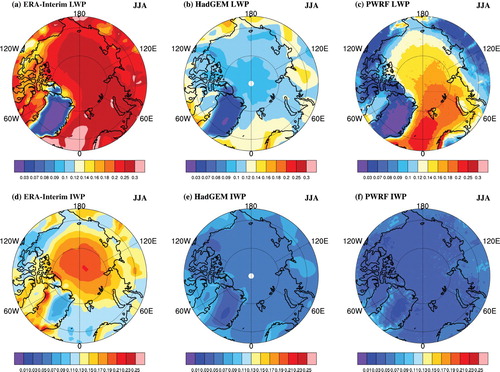
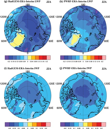
Compared with ERA-Interim data, the Polar WRF results (Fig. 10c) capture the dominant LWP spatial patterns exhibited by ERA-Interim (Fig. 10a) with the magnitudes underestimated (Fig. 10h), whereas HadGEM-ES2 does not simulate either the patterns or the magnitudes of LWP as well (Figs 10b and 10g). In addition, both models fail to simulate the IWP patterns and significantly underestimate the magnitudes shown by ERA-Interim in the Arctic basin (Figs 10d and 10f, and 10i and 10j). By comparison, in both the HadGEM-ES2 and Polar WRF results, the spatial patterns of the SWD_SFC and the LWD_SFC (Figs 9e and 9h, and Figs 9f and 9i) in the Arctic basin are similar to the LWP patterns (Figs 10b and 10c). This suggests the dominant impacts of LWP on SWD_SFC and LWD_SFC in both models, as shown in the ERA-Interim data. Too little LWP (Fig. 10g) and IWP (Fig. 10i) in the results from HadGEM-ES2 could lead to excesses in incident shortwave radiation over the Arctic basin and deficits in downward longwave radiation. Because of its improved simulation of LWP, Polar WRF more successfully captures the LWP-like patterns of SWD_SFC and the LWD_SFC when compared with ERA-Interim data than do HadGEM-ES2 results.

We note that although the simulations of LWP and IWP from Polar WRF are underestimated compared with ERA-Interim data, the results for SWD_SFC are still underestimated, whereas the LWD_SFC results are overestimated on the Atlantic side of the Arctic over open water. This suggests that other cloud radiative factors, including the height (or temperature) of the cloud base and the droplet size distribution, could play roles in the emissive and transmissive effects of the atmospheric column (Curry et al., 1996; Shupe & Intrieri, 2004). An additional consideration is that the different parameterizations of cloud radiative effects in the radiation schemes could also contribute to the different estimations of downward radiation at the surface in both models.

The difference in the LWP and IWP in the two model simulations could arise from different cloud physics and planetary boundary layer (PBL) schemes (Otkin & Greenwald, 2008), as well as the storms resolved in the two models. For cloud physics, Polar WRF employs the Morrison et al. (2005) bulk microphysics scheme, which consists of a two-moment formulation for cloud ice, cloud liquid, rain, snow, and graupel and predicts both the number concentration and the mixing ratio of cloud species. This new scheme is more realistic than previous formulations and is being developed and tested for the Arctic (e.g., Hines et al., 2015; Morrison, Pinto, Curry, & McFarquhar, 2008). Also, the associated MYJ PBL scheme (Janjić, 1994) is a non-singular implementation of the Mellor and Yamada (1982) level 2.5 turbulence closure model. By comparison, HadGEM-ES2 uses relatively simple large-scale physics parameterizations (Martin et al., 2006) in which the cloud microphysics scheme is a single moment scheme that explicitly predicts the mixing ratio of each hydrometeor species, and the boundary layer scheme is a first-order turbulence closure, with mixing of adiabatically conserved variables.

Besides these differences in the physical parameterizations, the notable improvement in LWP by Polar WRF, compared with HadGEM-ES2, is linked to its better simulation of synoptic cyclone densities and intensities and their resulting eddy transport of heat and water vapour toward the polar region. The LWP spatial pattern (Fig. 10a) resembles the distribution of moisture flux due to both stationary and transient components, in which the latter are dominant (Oshima & Yamazaki, 2004). There are three strong moisture inflows into the Arctic Ocean in summer: the two primary inflows from the North Atlantic and North Pacific and a third from central Eurasia due to transient flux (Oshima & Yamazaki, 2004; Overland, Turet, & Oort, 1996; Serreze et al., 1995). Corresponding to these three major inflows, there are significant point-to-point correlations between LWP and cyclone track density based on the 72 summer months (June to August) shown in the ERA-Interim data (Fig. 11a). Qualitatively similar correlation patterns can be seen in Polar WRF results (Fig. 11c). However, the correlations in the HadGEM2-ES simulation are poor, especially over the Laptev, Siberian, Chukchi, and Beaufort Seas, mostly due to the underestimated cyclonic systems. Moreover, there are significant correlations between LWP and the cyclone intensities over the North Atlantic side of the Arctic and the Chukchi and Beaufort Seas, as shown in ERA-Interim data (Fig. 11d). They are basically captured in Polar WRF results (Fig. 11f) but are underestimated in the HadGEM2-ES results over the Arctic and the Pacific sectors (Fig. 11e).

Fig. 11 Point-to-point correlation between liquid water path (LWP; kg m⁻²) with cyclone track density in summer (June–August; JJA) for the period 1979–2004 derived from (a) ERA-Interim, (b) HadGEM2-ES, and (c) Polar WRF data; (d) to (f) as in (a) to (c) but for the liquid water path (LWP, kg m⁻²) correlated with the central pressure of the cyclones.

5 Discussion and summary

In this study, we conducted a simulation of the Arctic climatology using a relatively fine-resolution regional atmospheric model, Polar WRF3.6, driven by outputs from the coarse-resolution climate model HadGEM-ES2, following the Fifth Assessment Report of the Intergovernmental Panel on Climate Change climate experiments. We presented the simulation of Arctic cyclone climatology from Polar WRF results during the historical period 1979–2004 in comparison with the parent model HadGEM-ES2 and the relatively fine-resolution ERA-Interim reanalysis data. Compared with the ERA-Interim data, HadGEM2-ES results underestimate cyclone frequency and intensity in the Arctic basin. By comparison, Polar WRF greatly improves the simulation of cyclone frequency, intensity, and size distribution over the Arctic basin, in both the cold and warm seasons. Both HadGEM2-ES and Polar WRF models simulate 13.2% fewer cyclone tracks in cold months than the ERA-Interim reanalysis. But Polar WRF produces more cyclones in the Beaufort, Barents, and Kara Seas and fewer in the East Greenland Sea than HadGEM2-ES and agrees more closely with ERA-Interim. Moreover, Polar WRF results are comparable with the cyclone intensities suggested by ERA-Interim data, which have (on average) central pressures about 10 hPa lower along the individual cyclone tracks, compared with HadGEM2-ES results. In the warm season, Polar WRF captures 10.5% more cyclone tracks than HadGEM2-ES although both models underestimate the Arctic cyclone tracks compared with ERA-Interim data. This improved performance can be partially attributed to better simulation of cyclogenesis and cyclolysis densities by Polar WRF in comparison with HadGEM2-ES results. In terms of intensity and size of cyclones in the Arctic Ocean, Polar WRF captures more intense cyclones, as well as more small cyclones than HadGEM2-ES, in better agreement with the ERA-Interim data.

Improved simulations of the Arctic synoptic weather systems lead to improved simulations of atmospheric surface fields. Because the monthly SLP and surface wind fields actually reflect the mean synoptic weather systems, overestimates of the Beaufort High in HadGEM-ES2 results are associated with fewer cyclones over the Beaufort Sea compared with ERA-Interim data. Similarly, the underestimated summer low over the central Arctic is related to fewer cyclones in both HadGEM-ES2 and Polar WRF simulations. Because of improved physics and increased horizontal resolution, Polar WRF tends to simulate cyclones that are smaller in size and stronger in surface wind speed compared with those simulated by a coarse-resolution GCM.

We have also shown that Polar WRF improves the simulation of surface radiation fields, partly because of an improved estimation of LWP. Compared with ERA-Interim data, in summer (June, July, and August), the HadGEM-ES2 results overestimate the absorbed solar radiation at the surface (negative in our convention) by as much as 30 W m⁻² in the Arctic basin and underestimate the longwave radiation by about 10 W m⁻². In contrast, Polar WRF compares well with ERA-Interim data in both spatial patterns and magnitudes. The differences in SW_SFC between the two models are a result of biases in SWD_SFC, which can be partially attributed to differences in LWP. Too little LWP and IWP in results from HadGEM-ES2 lead to excesses in incident shortwave radiation over the Arctic basin and deficits in LWD_SFC. Although Polar WRF also underestimates the IWP over the central Arctic, Polar WRF captures the LWP-like pattern of SWD_SFC more successfully than does HadGEM-ES2 when compared with ERA-Interim data because of its improved simulation of LWP. Likewise, owing to Polar WRF’s improved simulation of LWP, the resulting LWD_SFC estimates are also in better agreement with results from ERA-Interim than with results from HadGEM-ES2. The significantly improved LWP simulation by Polar WRF is linked to better simulation of the density and intensity of synoptic cyclones and their associated eddy transport of heat and water vapour toward the polar region from the North Atlantic, North Pacific, and central Eurasia.

Our study demonstrates the advantages of dynamic downscaling using Polar WRF to generate higher resolution estimates from the outputs of the climate model HadGEM-ES2. We also show the link between atmospheric Arctic cyclones and the energy budget of the Arctic basin. It is noteworthy, from the perspective of the absorbed solar radiation, for example, that the excessive gains in solar radiation in the Arctic basin can be related to underestimates in Arctic cyclone activity in HadGEM-ES2 results. In addition, it should be pointed out that there is possible uncertainty in the absolute total number of cyclones and statistical properties, partly related to their sensitivity to different track schemes (Neu et al., 2013; Rudeva, Gulev, Simmonds, & Tilinina, 2014; Ulbrich et al., 2013). With declining sea ice and increasing open water in the Arctic Ocean, the interactions between Arctic cyclones and the open ocean near the marginal ice zone are becoming increasingly important. Coupled atmosphere–ocean dynamics are a key factor (Long & Perrie, 2012). Therefore, it is necessary to establish a high-resolution coupled model system to study the effects and mechanisms of cyclones on the Arctic Ocean and sea ice, for example, diabatic heating over the open water and related climate impacts and related processes.

Acknowledgements

We thank anonymous reviewers for providing valuable comments that have helped improve our manuscript.

Disclosure statement

No potential conflict of interest was reported by the authors.

Additional information

Funding

Funding support was obtained from Canada’s Program on Energy Research and Development, the Canadian Marine Environmental Observation Prediction and Response (MEOPAR), the US Office of Naval Research, Award N00014-15-1-2611, and Fisheries and Oceans Canada's Aquatic Climate Change Adaptation Service Program (ACCASP).

References

- Béguin, A., Martius, O., Sprenger, M., Spichtinger, P., Folini, D., & Wernli, H. (2013). Tropopause level Rossby wave breaking in the northern hemisphere: A feature-based validation of the ECHAM5-HAM climate model. International Journal of Climatology, 33(14), 3073–3082. doi: 10.1002/joc.3631
- Blender, R., & Shubert, M. (2000). Cyclone tracking in different spatial and temporal resolutions. Monthly Weather Review, 128, 377–384. doi: 10.1175/1520-0493(2000)128<0377:CTIDSA>2.0.CO;2
- Boeke, R. C., & Taylor, P. C. (2016). Evaluation of the Arctic surface radiation budget in CMIP5 models. Journal of Geophysical Research, 121(14), 8525–8548. doi: 10.1002/2016JD025099
- Bromwich, D. H., Hines, K. M., & Bai, L.-S. (2009). Developments and testing of Polar Weather Research and Forecasting model: 2. Arctic Ocean. Journal of Geophysical Research, 114, D08122. doi: 10.1029/2008JD010300
- Cavallo, S. M., & Hakim, G. J. (2012). Radiative impact on tropopause polar vortices over the Arctic. Monthly Weather Review, 140(5), 1683–1702. doi: 10.1175/MWR-D-11-00182.1
- Cavallo, S. M., & Hakim, G. J. (2013). Physical mechanisms of tropopause polar vortex intensity change. Journal of the Atmospheric Sciences, 70(11), 3359–3373. doi: 10.1175/JAS-D-13-088.1
- Ceppi, P., Hartmann, D. L., & Webb, M. J. (2016). Mechanisms of the negative shortwave cloud feedback in middle to high latitudes. Journal of Climate, 29(1), 139–157. doi: 10.1175/JCLI-D-15-0327.1
- Collins, W. J., Bellouin, N., Doutriaux-Boucher, M., Gedney, N., Halloran, P., Hinton, T., … Martin, G. (2011). Development and evaluation of an Earth-system model–HadGEM2. Geoscientific Model Development, 4(4), 1051–1075. doi: 10.5194/gmd-4-1051-2011
- Condron, A., Bigg, G. R., & Renfrew, I. A. (2006). Polar mesoscale cyclones in the northeast Atlantic: Comparing climatologies from ERA-40 and satellite imagery. Monthly Weather Review, 134(5), 1518–1533. doi: 10.1175/MWR3136.1
- Curry, J. A., Schramm, J. L., Rossow, W. B., & Randall, D. (1996). Overview of Arctic cloud and radiation characteristics. Journal of Climate, 9(8), 1731–1764. doi: 10.1175/1520-0442(1996)009<1731:OOACAR>2.0.CO;2
- Dee, D. P., Uppala, S. M., Simmons, A. J., Berrisford, P., Poli, P., Kobayashi, S., … Bechtold, P. (2011). The ERA-Interim reanalysis: Configuration and performance of the data assimilation system. Quarterly Journal of the Royal Meteorological Society, 137, 553–597. doi: 10.1002/qj.828
- Denis, B., Laprise, R., & Caya, D. (2003). Sensitivity of a regional climate model to the spatial resolution and temporal updating frequency of lateral boundary conditions. Climate Dynamics, 20, 107–126. doi: 10.1007/s00382-002-0264-6
- Giorgi, F., & Mearns, L. O. (1991). Approaches to the simulation of regional climate change: A review. Reviews of Geophysics, 29, 191–216. doi: 10.1029/90RG02636
- Glisan, J. M., Gutowski Jr, W. J., Cassano, J. J., & Higgins, M. E. (2013). Effects of spectral nudging in WRF on Arctic temperature and precipitation simulations. Journal of Climate, 26(12), 3985–3999. doi: 10.1175/JCLI-D-12-00318.1
- Gregory, D., & Rowntree, P. R. (1990). A mass flux convection scheme with representation of cloud ensemble characteristics and stability-dependent closure. Monthly Weather Review, 118, 1483–1506. doi: 10.1175/1520-0493(1990)118<1483:AMFCSW>2.0.CO;2
- Grell, G. A., & Dévényi, D. (2002). A generalized approach to parameterizing convection combining ensemble and data assimilation techniques. Geophysical Research Letters, 29(14), 38-1–38-4. doi: 10.1029/2002GL015311
- Guo, L., Perrie, W., Long, Z., Chassé, J., Zhang, Y., & Huang, A. (2013). Dynamical downscaling over the Gulf of St. Lawrence using the Canadian regional climate model. Atmosphere-Ocean, 51(3), 265–283. doi: 10.1080/07055900.2013.798778
- Hines, K. M., & Bromwich, D. H. (2008). Development and testing of Polar Weather Research and Forecasting (WRF) model. Part I: Greenland Ice Sheet meteorology. Monthly Weather Review, 136, 1971–1989. doi: 10.1175/2007MWR2112.1
- Hines, K. M., Bromwich, D. H., Bai, L., Bitz, C. M., Powers, J. G., & Manning, K. W. (2015). Sea ice enhancements to Polar WRF. Monthly Weather Review, 143(6), 2363–2385. doi: 10.1175/MWR-D-14-00344.1
- Hines, K. M., Bromwich, D. H., Bai, L.-S., Barlage, M., & Slater, A. G. (2011). Development and testing of Polar WRF. Part III: Arctic land. Journal of Climate, 24, 26–48. doi: 10.1175/2010JCLI3460.1
- Huang, Y., & Zhang, M. (2014). The implication of radiative forcing and feedback for meridional energy transport. Geophysical Research Letters, 41(5), 1665–1672. doi: 10.1002/2013GL059079
- Janjić, Z. I. (1994). The step-mountain eta coordinate model: Further developments of the convection, viscous sublayer, and turbulence closure schemes. Monthly Weather Review, 122(5), 927–945. doi: 10.1175/1520-0493(1994)122<0927:TSMECM>2.0.CO;2
- Jung, T., Gulev, S. K., Rudeva, I., & Soloviov, V. (2006). Sensitivity of extratropical cyclone characteristics to horizontal resolution in the ECMWF model. Quarterly Journal of the Royal Meteorological Society, 132, 1839–1857. doi: 10.1256/qj.05.212
- Kay, J. E., & L’Ecuyer, T. (2013). Observational constraints on Arctic Ocean clouds and radiative fluxes during the early 21st century. Journal of Geophysical Research: Atmospheres, 118(13), 7219–7236.
- Ledrew, E. F. (1984). The role of local heat sources in synoptic activity within the polar basin. Atmosphere-Ocean, 22, 309–327. doi: 10.1080/07055900.1984.9649201
- Ledrew, E. F. (1988). Development processes for five depression systems within the polar basin. Journal of Climatology, 8, 125–153. doi: 10.1002/joc.3370080203
- Lock, A. P., Brown, A. R., Bush, M. R., Martin, G. M., & Smith, R. N. B. (2000). A new boundary layer mixing scheme. Part I: Scheme description and single-column model tests. Monthly Weather Review, 128, 3187–3199. doi: 10.1175/1520-0493(2000)128<3187:ANBLMS>2.0.CO;2
- Long, Z., & Perrie, W. (2012). Air-sea interactions during an Arctic storm. Journal of Geophysical Research: Atmospheres, 117(D15). doi: 10.1029/2011JD016985
- Long, Z., Perrie, W., Gyakum, J., Laprise, R., & Caya, D. (2009). Scenario changes in the climatology of winter midlatitude cyclone activity over eastern North America and the Northwest Atlantic. Journal of Geophysical Research: Atmospheres, 114(D12), 565. doi: 10.1029/2008JD010869
- Lubin, D., & Vogelmann, A. M. (2011). The influence of mixed-phase clouds on surface shortwave irradiance during the Arctic spring. Journal of Geophysical Research: Atmospheres, 116(D1), D00T05. doi: 10.1029/2011JD015761
- Martin, G. M., Ringer, M. A., Pope, V. D., Jones, A., Dearden, C., & Hinton, T. J. (2006). The physical properties of the atmosphere in the new Hadley Centre Global Environmental Model (HadGEM1). Part I: Model description and global climatology. Journal of Climate, 19(7), 1274–1301. doi: 10.1175/JCLI3636.1
- Massey, F. J. (1951). The Kolmogorov-Smirnov test for goodness of fit. Journal of the American Statistical Association, 46(253), 68–78. doi: 10.1080/01621459.1951.10500769
- Mellor, G. L., & Yamada, T. (1982). Development of a turbulence closure model for geophysical fluid problems. Reviews of Geophysics, 20(4), 851–875. doi: 10.1029/RG020i004p00851
- Morrison, H., Curry, J. A., & Khvorostyanov, V. I. (2005). A new double-moment microphysics parameterization for application in cloud and climate models. Part I: Description. Journal of the Atmospheric Sciences, 62, 1665–1677. doi: 10.1175/JAS3446.1
- Morrison, H., Pinto, J. O., Curry, J. A., & McFarquhar, G. M. (2008). Sensitivity of modeled Arctic mixed-phase stratocumulus to cloud condensation and ice nuclei over regionally varying surface conditions. Journal of Geophysical Research: Atmospheres, 113, D05203. doi: 10.1029/2007JD008729
- Murray, R. J., & Simmonds, I. (1991). A numerical scheme for tracking cyclone centres from digital data. Part I: Development and operation of the scheme. Australian Meteorology Magazine, 39, 155–166.
- Murray, R. J., & Simmonds, I. (1995). Responses of climate and cyclones to reductions in Arctic winter sea ice. Journal of Geophysical Research, 100(C3), 4791–4806. doi: 10.1029/94JC02206
- Neu, U., Akperov, M. G., Bellenbaum, N., Benestad, R., Blender, R., Caballero, R., … Wernli, H. (2013). IMILAST: A community effort to intercompare extratropical cyclone detection and tracking algorithms. Bulletin of the American Meteorological Society, 94(4), 529–547. doi: 10.1175/BAMS-D-11-00154.1
- Nishii, K., Nakamura, H., & Orsolini, Y. J. (2015). Arctic summer storm track in CMIP3/5 climate models. Climate Dynamics, 44(5-6), 1311–1327. doi: 10.1007/s00382-014-2229-y
- Ono, J., Inoue, J., Yamazaki, A., Dethloff, K., & Yamaguchi, H. (2016). The impact of radiosonde data on forecasting sea-ice distribution along the Northern Sea Route during an extremely developed cyclone. Journal of Advances in Modeling Earth Systems, 122(2), 775–787.
- Oshima, K., & Yamazaki, K. (2004). Seasonal variation of moisture transport in polar regions and the relation with annular modes. Polar Meteorology and Glaciology, 18, 30–53.
- Otkin, J. A., & Greenwald, T. J. (2008). Comparison of WRF model-simulated and MODIS-derived cloud data. Monthly Weather Review, 136(6), 1957–1970. doi: 10.1175/2007MWR2293.1
- Overland, J. E., Turet, P., & Oort, A. H. (1996). Regional variations of moist static energy flux into the Arctic. Journal of Climate, 9, 54–65. doi: 10.1175/1520-0442(1996)009<0054:RVOMSE>2.0.CO;2
- Parkinson, C. L., & Comiso, J. C. (2013). On the 2012 record low Arctic sea ice cover: Combined impact of preconditioning and an August storm. Geophysical Research Letters, 40, 1356–1361. doi: 10.1002/grl.50349
- Pezza, A. B., Simmonds, I., & Renwick, J. A. (2007). Southern hemisphere cyclones and anticyclones: Recent trends and links with decadal variability in the Pacific Ocean. International Journal of Climatology, 27(11), 1403–1419. doi: 10.1002/joc.1477
- Porter, D. F., Cassano, J. J., & Serreze, M. C. (2011). Analysis of the Arctic atmospheric energy budget in WRF: A comparison with reanalyses and satellite observations. Journal of Geophysical Research: Atmospheres, 116, D22108. doi: 10.1029/2011JD016622
- Raible, C. C., Della-Marta, P. M., Schwierz, C., Wernli, H., & Blender, R. (2008). Northern hemisphere extratropical cyclones: A comparison of detection and tracking methods and different reanalyses. Monthly Weather Review, 136, 880–897. doi: 10.1175/2007MWR2143.1
- Rayner, N. A., Parker, D. E., Horton, E. B., Folland, C. K., Alexander, L. V., Rowell, D. P., … Kaplan, A. (2003). Global analyses of sea surface temperature, sea ice, and night marine air temperature since the late nineteenth century. Journal of Geophysical Research, 108(D14), 4407. doi: 10.1029/2002JD002670
- Reed, R. J. (1979). Cyclogenesis in polar air streams. Monthly Weather Review, 107(1), 38–52. doi: 10.1175/1520-0493(1979)107<0038:CIPAS>2.0.CO;2
- Rudeva, I., Gulev, S. K., Simmonds, I., & Tilinina, N. (2014). The sensitivity of characteristics of cyclone activity to identification procedures in tracking algorithms. Tellus A: Dynamic Meteorology and Oceanography, 66, 24961. doi: 10.3402/tellusa.v66.24961
- Screen, J. A., Deser, C., Simmonds, I., & Tomas, R. (2014). Atmospheric impacts of Arctic sea-ice loss, 1979–2009: Separating forced change from atmospheric internal variability. Climate Dynamics, 43(1-2), 333–344. doi: 10.1007/s00382-013-1830-9
- Screen, J. A., Simmonds, I., Deser, C., & Tomas, R. (2013). The atmospheric response to three decades of observed Arctic sea ice loss. Journal of Climate, 26, 1230–1248. doi: 10.1175/JCLI-D-12-00063.1
- Screen, J. A., Simmonds, I., & Keay, K. (2011). Dramatic interannual changes of perennial Arctic sea ice linked to abnormal summer storm activity. Journal of Geophysical Research, 116, C00A06. doi: 10.1029/2011JD015847
- Serreze, M. C. (1995). Climatological aspects of cyclone development and decay in the Arctic. Atmosphere-Ocean, 33(1), 1–23. doi: 10.1080/07055900.1995.9649522
- Serreze, M. C., & Barrett, A. P. (2008). The summer cyclone maximum over the central Arctic Ocean. Journal of Climate, 21(5), 1048–1065. doi: 10.1175/2007JCLI1810.1
- Serreze, M. C., & Barry, R. G. (2005). The Arctic climate system. Cambridge: Cambridge University Press.
- Serreze, M. C., Barry, R. G., Rehder, M. C., Walsh, J. E., & Drewry, D. (1995). Variability in atmospheric circulation and moisture flux over the Arctic [and discussion]. Philosophical Transactions of the Royal Society A: Mathematical, Physical and Engineering Sciences, 352(1699), 215–225.
- Shkolnik, I. M., & Efimov, S. V. (2013). Cyclonic activity in high latitudes as simulated by a regional atmospheric climate model: Added value and uncertainties. Environmental Research Letters, 8, 045007. doi: 10.1088/1748-9326/8/4/045007
- Shupe, M. D., & Intrieri, J. M. (2004). Cloud radiative forcing of the Arctic surface: The influence of cloud properties, surface albedo, and solar zenith angle. Journal of Climate, 17, 616–628. doi: 10.1175/1520-0442(2004)017<0616:CRFOTA>2.0.CO;2
- Simmonds, I. (2000). Size changes over the life of sea level cyclones in the NCEP reanalysis. Monthly Weather Review, 128(12), 4118–4125. doi: 10.1175/1520-0493(2000)129<4118:SCOTLO>2.0.CO;2
- Simmonds, I. (2015). Comparing and contrasting the behaviour of Arctic and Antarctic sea ice over the 35 year period 1979–2013. Annals of Glaciology, 56(69), 18–28. doi: 10.3189/2015AoG69A909
- Simmonds, I., Burke, C., & Keay, K. (2008). Arctic climate change as manifest in cyclone behavior. Journal of Climate, 21(22), 5777–5796. doi: 10.1175/2008JCLI2366.1
- Simmonds, I., & Keay, K. (2009). Extraordinary September Arctic sea ice reductions and their relationships with storm behavior over 1979–2008. Geophysical Research Letters, 36, 4045. doi: 10.1029/2009GL039810
- Simmonds, I., & Rudeva, I. (2012). The great Arctic cyclone of August 2012. Geophysical Research Letters, 39, L23709. doi: 10.1029/2012GL054259
- Simmonds, I., & Rudeva, I. (2014). A comparison of tracking methods for extreme cyclones in the Arctic basin. Tellus A: Dynamic Meteorology and Oceanography, 66(1), 25252. doi: 10.3402/tellusa.v66.25252
- Simmons, A., Uppala, S., Dee, D., & Kobayashi, S. (2007). ERA-Interim: New ECMWF reanalysis products from 1989 onwards. ECMWF Newsletter, 110(110), 25–35.
- Smith, R. N. B., D. Gregory, C. A. Wilson, Bushell, A. C., & Cusack, S. (1999). Calculation of saturated specific humidity and largescale cloud. UM Documentation Paper 29. Exeter: Met Office.
- Stephens, G. L. (1978). Radiation profiles in extended water clouds. I: Theory. Journal of the Atmospheric Sciences, 35(11), 2111–2122. doi: 10.1175/1520-0469(1978)035<2111:RPIEWC>2.0.CO;2
- Stroeve, J., Holland, M. M., Meier, W., Scambos, T., & Serreze, M. (2007). Arctic sea ice decline: Faster than forecast. Geophysical Research Letters, 34, 3498. doi: 10.1029/2007GL029703
- Tanaka, H. L., Yamagami, A., & Takahashi, S. (2012). The structure and behavior of the Arctic cyclone in summer analyzed by the JRA-25/JCDAS data. Polar Science, 6(1), 55–69. doi: 10.1016/j.polar.2012.03.001
- Tilinina, N., Gulev, S. K., & Bromwich, D. H. (2014). New view of Arctic cyclone activity from the Arctic system reanalysis. Geophysical Research Letters, 41, 1766–1772. doi: 10.1002/2013GL058924
- Ulbrich, U., Leckebusch, G. C., Grieger, J., Schuster, M., Akperov, M., Bardin, M. Y., … Kew, S. F. (2013). Are greenhouse gas signals of northern hemisphere winter extra-tropical cyclone activity dependent on the identification and tracking algorithm? Meteorologische Zeitschrift, 22(1), 61–68. doi: 10.1127/0941-2948/2013/0420
- Uotila, P., Pezza, A. B., Cassano, J. J., Keay, K., & Lynch, A. H. (2009). A comparison of low pressure system statistics derived from a high-resolution NWP output and three reanalysis products over the Southern Ocean. Journal of Geophysical Research, 114, 3518. doi: 10.1029/2008JD011583
- Wang, Y., Leung, L., McGregor, J., Lee, D., Wang, W., Ding, Y., & Kimura, F. (2004). Regional climate modeling: Progress, challenges, and prospects. Journal of the Meteorological Society of Japan. Series II, 82(6), 1599–1628. doi: 10.2151/jmsj.82.1599
- Yamazaki, A., Inoue, J., Dethloff, K., Maturilli, M., & König-Langlo, G. (2015). Impact of radiosonde observations on forecasting summertime Arctic cyclone formation. Journal of Geophysical Research: Atmospheres, 120(8), 3249–3273.
- Zhang, J., Lindsay, R., Schweiger, A., & Steele, M. (2013). The impact of an intense summer cyclone on 2012 Arctic sea ice retreat. Geophysical Research Letters, 40(4), 720–726. doi: 10.1002/grl.50190
- Zhang, J., Lindsay, R., Steele, M., & Schweiger, A. (2008). What drove the dramatic retreat of Arctic sea ice during summer 2007. Geophysical Research Letters, 35(11), L18504. doi: 10.1029/2008GL034005
- Zhang, X., Walsh, J. E., Zhang, J., Bhatt, U. S., & Ikeda, M. (2004). Climatology and interannual variability of Arctic cyclone activity: 1948–2002. Journal of Climate, 17, 2300–2317. doi: 10.1175/1520-0442(2004)017<2300:CAIVOA>2.0.CO;2