Prediction of the South China Sea Dipole Using SSA-MEM

ABSTRACT

A dipole structure appears in the sea surface height off the central coast of Vietnam during boreal summer in the South China Sea. This dipole, which possesses a chlorophyll signature associated with higher phytoplankton concentrations arising from nutrient upwelling, is important for the productivity of local fisheries. Multi-satellite sea level anomalies are used to investigate the life cycle of the dipole structure. By applying empirical orthogonal function (EOF) analysis, the third EOF mode (EOF 3) is found to represent the major variations of the dipole structure. By removing the temporal noise of EOF 3, a South China Sea dipole index is defined. This index captures the life cycle of the dipole including its generation, mature strength, and final termination. Both one-dimensional and two-dimensional forecasts are generated using a statistical forecasting method that combines singular-spectrum analysis and the maximum entropy method. The appearance of the dipole structure can be predicted with an accuracy of 78% at one-month lead times and an accuracy of 61% at one-year lead times.

Résumé

[Traduit par la rédaction] Une structure en dipôle apparaît dans la hauteur de la surface de la mer au large de la côte centrale du Vietnam, durant l’été boréal, dans la mer de Chine méridionale. Ce dipôle, qui possède une signature de chlorophylle correspondant à des concentrations accrues de phytoplancton qui résultent de la remontée de nutriments, revêt de l’importance pour la productivité des pêcheries locales. Nous utilisons les anomalies de niveaux marins provenant de mesures qu’ont enregistrées de multiples satellites pour étudier le cycle de vie de ce dipôle. En analysant les données à l’aide de fonctions orthogonales empiriques, nous déterminons que le troisième mode représente les variations principales de la structure du dipôle. Nous définissons un indice du dipôle de la mer de Chine méridionale en retirant le bruit temporel du troisième mode. Cet indice reflète le cycle de vie du dipôle, y compris sa genèse, son intensité à maturité et son déclin. Nous générons des prévisions unidimensionnelles et bidimensionnelles à l’aide d’une méthode de prévision statistique qui combine l’analyse spectrale singulière et la méthode d’entropie maximale. Nous pouvons ainsi prévoir un mois d’avance et avec une précision de 78% la formation du dipôle, et le faire un an d’avance avec une précision de 61%.

KEYWORDS:

• South China Sea
• sea level dipole structure
• SSA-MEM
• statistical prediction

1 Introduction

Ocean mesoscale eddies, with typical horizontal scales of less than 100 km and time scales on the order of one month, are the “weather” of the ocean. They are ubiquitous, coherent, rotating structures that typically exhibit water properties different from their surroundings, which allows them to transport properties such as heat, salt, and carbon around the ocean. The fact that the water contained within eddies is often enriched with nutrients implies that they may be an important source of nutrients for coastal zones and the surface ocean and may feed the plankton blooms that often occur. Oceanic transports of heat, salt, fresh water, dissolved CO₂, and other tracers regulate the distribution of natural marine resources and impact global climate change. More than half the kinetic energy of the upper ocean circulation is contained in the mesoscale eddy field, with the remainder being primarily contained in the large-scale general circulation. Although it remains a difficult challenge, accurate mesoscale eddy prediction is of great importance for understanding the energy budget of the ocean. In this paper, we attempt to forecast the South China Sea (SCS) dipole structure, a type of eddy that occurs in the Vietnamese coastal zone.

The SCS is a marginal sea of the western tropical Pacific Ocean, covering the area between 3°S, 23°N and 100°E, 120°E and possessing an average basin depth of more than 2000 m (Li et al., 2014). It is connected to the East China Sea to the northeast, the Pacific Ocean and the Sulu Sea to the east, and the Java Sea and the Indian Ocean to the southwest (Xie, Xie, Wang, & Liu, 2003). The circulation within the SCS has a strong annual cycle, and the seasonal variation of the SCS circulation is driven primarily by the monsoon. The basin-scale circulation of the upper SCS is generally cyclonic in boreal winter (boreal omitted hereafter) in response to the strong positive wind stress curl of the northeast monsoon and dominated by a double gyre in summer comprised of a northern cyclonic gyre, a southern anticyclonic gyre, and an eastward jet on the inter-gyre boundary between 11°N and 14°N (Bayler & Liu, 2008; Gan & Qu, 2008; Xie, Chang, Xi, & Wang, 2007). This summer circulation is driven by the Annam Cordillera impinging upon the southwest monsoon, which forces an atmospheric jet southeast of Ho Chi Minh City (Xie et al., 2003), creating a wind curl dipole that drives the double gyre in the ocean. The elevated sea surface height (SSH) anticyclonic gyre centred at 9°–10°N (Li et al., 2014) is larger in size than the low SSH cyclonic gyre centred near 13.5°N, 111°E off Vietnam.

The northern cyclonic and the southern anticyclonic gyres consitute the dipole structure, which is also called the Vietnam warm and cold eddy or the eddy pair (Chen, Hou, Zhang, & Chu, 2010). Wang, Chen, and Su (2006) and Chen, Hou, and Chu (2011) studied the life cycle of this dipole and determined that, on average, the dipole structure appears in June, amplifies through summer, reaches peak strength in August or September, weakens during October, and dissipates by the end of October. Wang et al. (2006) suggested that the eddy pair is a result of the two oppositely rotating wind-driven gyres, with the non-linear vorticity transports from the western boundary currents being crucial for the generation of the dipole structure. In the southern SCS, the net effect of the inertial process of the wind-driven southern gyre is to advect negative vorticity northward by its northward western boundary current, thereby concentrating negative vorticity at the northwest corner of the southern gyre to form the anticyclonic eddy. Likewise, in the northern SCS, the net effect of the inertial process of the wind-driven northern gyre is to advect positive vorticity southward by its southward western boundary current, concentrating positive vorticity into the southwest area of the northern gyre to form the cyclonic eddy. Such vorticity transports from the two western boundary currents result in the dipole structure off central Vietnam, with an eastward current jet in between. Because the dipole seems to be the result of two oppositely rotating wind-driven gyres, the wind field should be important for formation of the dipole. The strength of the wind stress curl is found to play an important role in the generation and maintenance of the dipole structure. Compared with the non-linearity effects, the input of vorticity from the wind stress curl is equally, if not more, important to the dipole structure. In addition, the strength and direction of the offshore wind jet also play a significant role in determining the magnitudes and core positions of the two eddies that make up the dipole (Wang et al., 2006).

Associated with these gyres is a strong coastal current. In summer, the prevailing southwest monsoon induces coastal upwelling and drives a northeastward flowing coastal current along the Vietnamese coast (Dippner, Nguyen, Hein, Ohde, & Loick, 2007; Li et al., 2014). The upwelling induced a drop in sea surface temperature (SST) of more than 1°C off the coast of Vietnam (Xie et al., 2003). The northeastward flowing Vietnam Coastal Current separates from the coast near 12°N and feeds an eastward flowing jet off central Vietnam (Li et al., 2014; Wang et al., 2006). The cold SST produced by coastal upwelling extends offshore and feeds water into a cold jet stretching eastward into the interior of the SCS (Kuo, Zheng, & Ho, 2000; Lian & Chen, 2012; Liu, Jiang, Xie, & Liu, 2004). The orographic-induced southwest atmospheric jet is key to the cold jet's offshore development, by inducing coastal upwelling and driving the eastward ocean jet that advects the cold coastal water offshore (Xie et al., 2003). This cold jet is important for the basin-scale SST, SCS ocean circulation, biological activity, and regional climate variability (Li et al., 2014; Xie et al., 2003).

The generation of the SCS dipole structure and associated cold jet can signal the rise of chlorophyll concentration along the Vietnamese coast, which has great significance for biological activity. Therefore, the ability to accurately predict the appearance and temporal evolution of the dipole structure can provide reliable marine information and better serve the aquaculture industry. Our study is the first to predict the life cycle of the SCS dipole structure. The dipole's life cycle has a strong periodicity tied to the annual cycle, making accurate prediction feasible. We present statistical forecasting of the dipole's evolution using an empirical time extrapolation method. Statistical forecasting methods have been widely applied to the prediction of the El Niño–Southern Oscillation (ENSO; Tangang, Tang, Monahan, & Hsieh, 1998; Xue, Leetmaa, & Ji, 2000), sea-ice coverage (Chen & Yuan, 2004), ocean monsoons (Wu, Yan, & Chen, 2013), and other ocean phenomena. To the best of our knowledge, no previous studies have attempted to predict the SCS dipole. This is probably because of the difficulty in making accurate predictions for systems that have a wide variety of physical processes acting over a broad range of spatial and temporal scales.

Our paper is organized as follows. Section 2 describes the data and methodology. Section 3 defines a dipole index and describes the details of the statistical prediction of the SCS dipole. The influence of ENSO on the dipole structure is also presented in Section 3. A discussion of the results is given in Section 4, followed by conclusions in Section 5.

2 Data and methodology

a Data

Gridded SSH anomaly data are obtained from the Archiving, Validation and Interpretation of Satellite Oceanographic (Aviso) program at the Centre national d’études spatiales in France. The sea level anomaly (SLA) data used in our study is from the Duacs 2014 version (V15.0) with a spatial resolution of 1/4° × 1/4°. The daily data span the time period 1 January 1993 to 10 March 2016 for the area 106°–116°E, 6°–18°N used in our study.

b Methods

1 eof

An empirical orthogonal function (EOF) analysis is an effective eigenvalue method for phenomenological identification and space reduction that is widely used in climate research (Lian & Chen, 2012). An EOF analysis separates the spatiotemporal field into spatial patterns that possess the most variance of a signal and their corresponding time sequences. In our study, EOF analysis is applied to the SLA data to obtain the dominant spatial patterns of the SCS dipole and their corresponding temporal evolutions.

2 ssa-mem

Singular-Spectrum Analysis (SSA) is a statistical method related to EOF analysis, but it is applied to noisy time series. A detailed description of SSA can be found in Ghil et al. (2002); however, a summary of the method is given here. The SSA method extracts as much reliable information as possible from short and noisy time series without prior knowledge of the dynamics of the underlying series. It is a form of principal component analysis applied to lag-correlation structures of uni- and multivariate time series. Using data-adaptive filters, SSA decomposes a time series into oscillatory, trending, and noise components; it generates statistically significant information based on these components and provides reconstructed signals based upon these components. In our study, we use SSA to extract the primary component of the time series of the third mode of the EOF (EOF 3 hereafter) and define it as a dipole index.

It has been shown that the application of a method combining SSA and the maximum entropy method (MEM) to a univariate indicator, such as the dipole index, can be helpful in extrapolating the time series. First, SSA is applied to the time series of the dipole index, which decomposes that time series into various components with various frequencies. Next, MEM is applied to advance these components in time. These extended components are then used for an SSA-reconstruction to produce the forecast values. The predictive power of the SSA-MEM method is mainly due to the ability of SSA to adaptively filter temporal oscillations in the presence of a large amount of noise (Keppenne, 1995).

3 Results

In this section, the dipole index is defined, and the life cycle of the indexed dipole is compared with the life cycle observed from SLA maps. The index construction is based on the EOF results for the SLA from the study area. By applying a statistical forecasting method, the time series can be extended to generate a prediction.

a EOF results

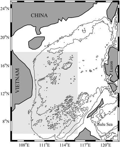
To focus on the signal from the dipole structure, only data from the area bounded by 106°–116°E, 6°–18°N are used in our study. Figure 1 shows the bathymetry of the SCS and the location of the study area (lightly shaded area).

Fig. 1 Map of the SCS (106°–122°E, 5°–25°N). The two contours are the 200 and 2000 m isobaths. The study area is indicated by light grey shading (106°–116°E, 6°–18°N).

We applied EOF analysis to data from the study area. Our study focuses on the first three EOF modes, which account for 66.7% of the total variance. They represent the main dynamical features of the study area. The spatial patterns of the first three EOF modes are presented in Fig. 2. The annual cycle of the basin-wide circulation is characterized by EOF modes 1 and 2. The time sequence of mode 2 (not shown) indicates that there is a sea level rise within the study area. The general features of the dipole structure are clearly captured by EOF 3, which accounts for 9.2% of the total variance.

Fig. 2 The first three EOF modes of SLA. EOFs 1, 2, and 3 represent 39.3, 18.2 and 9.2% of the total variance, respectively.

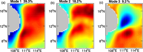
Because we wish to focus on the dipole pattern contained in EOF 3, EOF 1 and EOF 2 will not be discussed in detail here. The dipole pattern captured in EOF 3 consists of a cyclonic circulation in the north and an anticyclonic circulation in the south, and the time sequence of EOF 3 shows strong annual variation (Fig. 3).

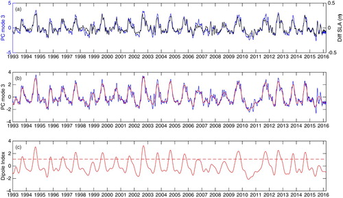
Fig. 3 (a) Time series of EOF 3 (blue) and the mean SLA difference (black) between Zone 1 (12°–15°N, 110°–112°E) and Zone 2 (8°–12°N, 111°–114°E). (b) Time series of EOF 3 (blue) and the reconstructed time sequence (red). (c) Time series of the dipole index (the dashed red line indicates the 1.1 threshold).

b Life cycle of the SCS dipole

First, a dipole index is defined from the SLA to provide an indicator of the strength of the dipole structure to enable its life cycle to be quantified. The life cycle of the SCS dipole as measured by altimeter observations is then compared with the life cycle as measured by the dipole index.

The normalized time series of EOF 3 is shown in Fig. 3a. For comparison, the mean SLA difference between two selected zones (Zone 1: 12°–15°N, 110°–112°E and Zone 2: 8°–12°N, 111°–114°E) is also shown. The high correlation (r² = 0.94) between the time series of EOF 3 and the mean SLA difference verifies the validity of defining the dipole index using the EOF 3 time sequence. Consequently, the dipole index is extracted by removing noise from the original time series and applying SSA (Fig. 3b). To ensure that the index successfully indicates the life cycle of the dipole, a threshold must be set. Therefore, in each year when the value of the dipole index first reaches the threshold value, the dipole is considered to have been generated. The index will continue to grow throughout the summer and then begin to decrease in late fall. When the value of the index first drops to the threshold value, after having reached a peak value, the dipole is considered to have died. The threshold value is chosen as the average of the index value at the time the dipole first appears or disappears. As with all indices, the value of the dipole index represents the strength of the dipole during its life cycle. Here the dipole strength is defined as the difference between the lowest central SLA of the cold eddy and the highest central SLA of the warm eddy.

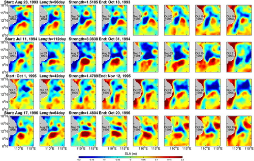
 Figure 4 presents SLA maps of the dipole structure for 1993 to 1996. The structures of the dipole on the generation and termination dates are labelled in the first and last columns, respectively. The lifespan (termination date minus generation date) and maximum strength (the local maximum value of the dipole index) of the dipole each year is also labelled in Fig. 4. The evolution of the dipole in each year can be clearly seen in Fig. 4. The cold eddy branch of the dipole originates mostly near the coast of Vietnam, except in some years when it originates from the inner SCS, then merges with the coastal water. Although the cold eddy appears in concert with the cold jet, the cold eddy persists even after the cold jet disappears. Following generation, the cold eddy initially propagates to the northeast, away from the coast, and amplifies. After roughly one or two months the cold eddy moves back to the coast, stretching into a long, narrow shape and merges with the Southwest Coastal Current. The warm eddy of the dipole often appears earlier than the cold eddy. Compared with the cold eddy, the location of the warm eddy seems more stable. When the cold eddy moves back to the coast and stretches into a long, narrow shape the warm eddy then moves northwestward with the southward coastal current and occupies the original location of the cold eddy.

Fig. 4 Interannual variability of the dipole life cycle characteristics from 1993 to 1996. Each row represents the evolution of the SLA from the dipole start date to the end date in each year. The title shows the start date, the lifetime, the strength, and the end date of the dipole detected by the dipole index.

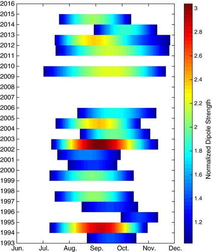
The life cycle of the dipole index from 1993 to 2015 is presented in Fig. 5. The dipole structure typically appears in July, peaks in September, and disappears in November. The dipole is strongly influenced by wind. The strength of the wind stress curl plays an important role in the generation and maintenance of the dipole structure. The input of vorticity from the wind stress curl is important to the dipole structure. It should be noted that in 1995, 1998, 2006, 2007, 2008, and 2010 there were no dipoles and the eastward cold jet shifted northward because of the northeasterly anomaly of the summer monsoon (Chen & Wang, 2014), and the monsoon which impacts the dipole is strongly related to ENSO. In 1994 and 2002, years during which an El Niño developed, two extremely strong dipoles occurred. We speculate that the wind stress curl was stronger than in normal years, which led to a stronger dipole (Wang, 2002). In 1998, 2007 and 2010, which were El Niño decaying years, the wind stress curl was too small for a dipole to be generated (Chu et al., 2014; Kuo, Zheng, & Ho, 2004).

Fig. 5 The life cycle of the dipole structure in each year (the colour bar indicates the strength of the dipole structure normalized by its standard deviation).

Table 1 lists the generation date, termination date, and maximum strength of the dipole inferred from daily SLA maps. We identify and track the evolution of the dipole according to the following three criteria: (i) cyclonic or anticyclonic eddies are deemed to exist when the difference between the absolute SLA at the eddy centre and that at the outermost closed contour line exceeds 6 cm; (ii) the dipole is considered to have been generated when both the cyclonic and anticyclonic eddies exist off the coast of Vietnam; and (iii) the dipole is deemed to terminate when either one of the eddies dissipates to a point where the SLA difference from centre to edge has decreased below 6 cm. Cyclonic and anticyclonic eddies are typically generated locally off the coast of Vietnam and can be easily tracked over the course of a month. However, it should be noted that in 1993, 2000, and 2001 the cold eddy was not generated off the coast of Vietnam as usual, rather it first appeared in the middle of the SCS then subsequently merged with the cold water off the Vietnamese coast. For these three years, we define the generation date as the day when the cold eddy first merged with upwelling cold water off the Vietnamese coast; otherwise, we could not unambiguously claim that this cold-core eddy was, in fact, the Vietnamese Cold Eddy of the dipole.

Table 1. The life cycle of the dipole over the past 23 years detected from daily SLA maps.

Year	Generation	Dipole Strength	Termination
1993	2 July	50.34	29 October
1994	8 July	71.36	28 October
1995	none	none	none
1996	16 August	54.53	8 November
1997	18 July	57.9	10 October
1998	none	none	none
1999	9 July	61.76	29 October
2000	11 August	56.84	6 October
2001	20 July	51.52	28 September
2002	19 July	69.71	15 November
2003	8 August	50.89	31 October
2004	23 July	55.43	15 October
2005	24 June	51.78	11 November
2006	none	none	none
2007	none	none	none
2008	none	none	none
2009	24 July	65.91	13 November
2010	none	none	none
2011	19 August	58.99	11 November
2012	20 July	61.21	16 November
2013	30 August	47.45	1 November
2014	25 July	54.56	24 October
2015	none	none	none

To confirm the utility of the dipole index, we compare the generation and termination dates detected from the daily SLA maps with those indicated by the dipole index. If the difference between the generation and termination dates from the SLA maps and the dipole index is less than two weeks, we consider the times detected by the dipole index to be sufficiently accurate. For more than three-quarters of the cases (∼78.3%), the dipole index accurately determines the generation and termination dates. However, there are some notable exceptions; for example, while there was no dipole structure observed in the SLA maps in 1995, the dipole index indicated a weak dipole that year. The dipole index can also be used to indicate the strength of the dipole by considering the magnitude of its local maxima. As mentioned before, the sea level difference between the maximum sea level of the warm-core eddy and the minimum sea level of the cold-core eddy is defined as the estimate of the dipole strength each year. The correlation coefficient between the maxima in the dipole index and the dipole strength is approximately 0.8, suggesting that the peak of the dipole index is an adequate predictor of the dipole strength each year.

c Forecast of the dipole structure

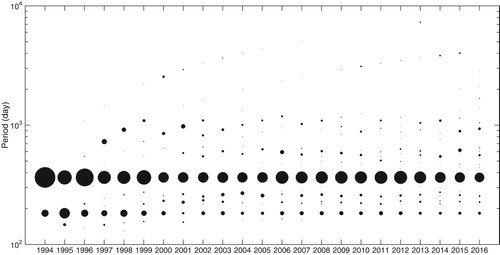
The fidelity of the statistical forecasting relies on the regularity of the time series. More regular time series lead to higher prediction accuracy. Therefore, before applying the prediction methodology, the regularity of the time series needs to be analyzed. Figure 6 shows a spectral analysis of the dipole indices as a function of the final year. The dipole index was decomposed into multiple quasi-periodic components using SSA. Details of SSA decomposition and reconstruction are presented below in Eqs (1) to (3). In Fig. 6 we can see two dominant oscillations embedded within the dipole index: one is the annual cycle, the other is the semi-annual oscillation. The forecast would be more accurate if only applied to each quasi-periodic component, but the forecast error will be amplified when each component is added together. Therefore, choosing the right method of decomposing the dipole index is essential to the forecast. In our study, before the forecast methodology is applied, the dipole index is decomposed into four quasi-periodic time series with different primary frequencies. The primary periods for the four quasi-periodic time series are 183 days, 183–365 days, 365 days, and longer than 365 days. With the dipole index decomposed into four time series with stronger periodicity, the statistical prediction is more accurate. The details of the procedure can be found in the following section.

Fig. 6 Spectral analysis of the dipole indices as a function of the final year (the radius of each dot is proportional to the variance of each component).

After decomposition, each quasi-periodic time series is subject to the forecasting methodology. To produce a forecast, one needs historical data before the forecast period. The length of the leading historical data time series is called the training period. For example, if we intend to forecast the dipole index for 2012, then the training period is 1 January 1993 to 31 December 2011. The methodology combines the SSA method with MEM to perform the statistical prediction. The leading SSA modes, which are orthogonal, are determined from the training period. The time series can be projected onto EOFs in a time domain (T-EOFs) to obtain the corresponding principal components (T-PCs). By summing the T-EOFs and related T-PCs the original fluctuation can be obtained, which is called the reconstruction. To produce the forecast, MEM is used to determine the autoregressive coefficients from the training period. These coefficients are then used to advance the T-PCs. The summation of T-EOFs and the advanced T-PCs gives the predicted dipole index. The SSA-MEM method is effective for any time series containing large oscillatory components. The deficiency of this method is that the forecast magnitudes of the anomalies are usually weaker than those typically observed (Mo, 2001).

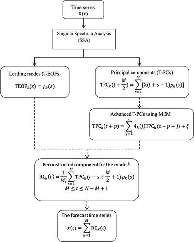
The major steps for the dipole forecast are illustrated in Fig. 7. Given a time series of length N, one can calculate the time-lagged covariance matrix up to lag , where is the window length. Details can be found in Ghil et al. (2002). The T-EOFs are the eigenfunctions of the symmetric matrix. The time series are projected onto the T-EOFs to obtain the corresponding principal components (T-PCs). The kth T-PC is given by:(1) where is the kth T-EOF. The total length of any given T-PC is . For each mode the time series can be reconstructed by adding T-EOF and the corresponding T-PC. The reconstructed component for mode will be referred to as :(2) where ; except near the endpoints ( or ), the summation in goes from 1 to or from to and . The summation of all of the will reconstruct the original time series:(3) For any time series the procedures above can be followed to obtain SSA modes and the related T-PCs.

Fig. 7 The flowchart of a forecast. is the time series that needs to be forecast; is the window length; is the length of time series ; is the forecast lead time; and is the order of the AR process. Solid and dashed arrows denote the training and forecast procedures, respectively.

After the SSA has been applied to each time series, MEM is used to generate the forecast. Each T-PC extracted by SSA is separately submitted to MEM to obtain the autoregression (AR) coefficients. In turn, the AR coefficients are used to advance the T-PC. One can extrapolate the jth T-PC based on by:(4)

where is a Gaussian white noise process with variance , is the forecast lead time, and is the order of the AR process. Order is given and fixed in the process. Further, is the jth AR coefficient for the kth T-PC. Burg's method is used (Burg, 1968) to determine the for to for the training period. This method, reviewed by Penland, Ghil, and Weickmann (1991), is a recursive method to solve for the AR coefficients by utilizing the symmetric Toeplitz matrix structure of the autocovariance matrix. After determining , the above equation is used to extrapolate the T-PC. The RCs can be reconstructed from T-PCs and the related T-EOFs. The summation of the RCs will give the predicted time series.

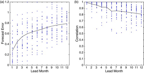
After predictions have been made for all four quasi-periodic time series, the forecast time series are added together to give the predicted dipole index. An example of the forecast time series and the predicted dipole index is shown in Fig. 8. The four quasi-periodic time series are RC1, RC2, RC3, and RC4, and the predicted dipole index is shown in the lower panel. To conduct an error analysis, we plot the forecast error and the correlation coefficient between the predicted and observed dipole indices as a function of lead time (Fig. 9). The forecast error is defined as the root mean square error between the predicted and original time series divided by the standard deviation of the predicted time series. The analysis is applied to 30 indices with different end times, and for each index the lead time varies from one month to one year. From Fig. 9 we can see that the average forecast error increases from 0.24 with one-month lead time to 0.79 with one-year lead time, and the correlation coefficient drops from 0.99 with one-month lead time to 0.81 with one-year lead time. Although the prediction accuracy decreases when lead time grows, the prediction accuracy is still high at one-year lead time.

Fig. 8 Statistical prediction for 2011. The upper four panels are the predictions of the four quasi-periodic time series, and the lower panel shows the prediction of the dipole index (the blue lines indicate the training period; the red lines are the predictions; the dashed black line in the lower panel is the prediction of the dipole index).

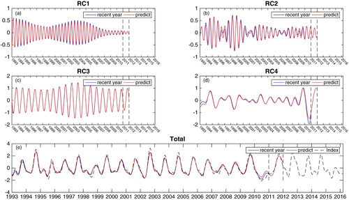
Fig. 9 (a) Forecast error estimate and (b) correlation coefficient of the predicted and observed dipole indices as a function of the lead time (in months, blue dots are the error for each forecast case; the black line indicates the average of all 30 cases).

d Two-dimensional forecast

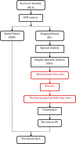
For a more visual forecast of the SCS dipole, a two-dimensional prediction is developed. The two-dimensional prediction is based on the ability of EOF analysis to separate the spatial pattern of the SLA field from its temporal evolution. Because the time series of each mode can be predicted independently, the two-dimensional forecast is given by the reconstruction of the SLA field using the original EOF spatial pattern and a prolonged EOF temporal pattern. The flowchart of the two-dimensional prediction methodology is shown in Fig. 10. The right arm of the flowchart shows the one-dimensional forecast used in Section 3.c.

Fig. 10 Flowchart of the two-dimensional forecast methodology (the procedure shown in the red boxes can be specialized to obtain the flowchart shown in Fig. 7).

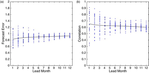
The first three EOF modes are used to predict the temporal evolution of the two-dimensional dipole structure in our study. The prediction was limited to these three modes because the time sequences of the other EOF modes have a weaker periodicity that will introduce significant forecast error. Figures 11 and 12 show the predicted SLA field with one-month lead time compared with the reconstructed SLA field and the original SLA field, respectively. The error estimate is shown in Figs 13 and 14. We conclude that the forecast accuracy is high for the reconstructed SLA field but is sharply reduced for the original SLA field. This is not too surprising, considering that the first three EOF modes only account for two-thirds (66.7%) of the total variance. To attempt to improve the prediction for the observed SLA field, we also used the first four and the first six EOF modes to make the prediction, but the results were not satisfactory because the temporal modes of EOF 4, EOF 5, and EOF 6 are too irregular to make an accurate prediction.

Fig. 11 Evolution of the reconstructed SLA field using the first three EOF modes (black) and the predicted SLA field with a one-month lead time (red) for 2011. Areas where the absolute value of the SLA field is larger than 0.1 are shaded.

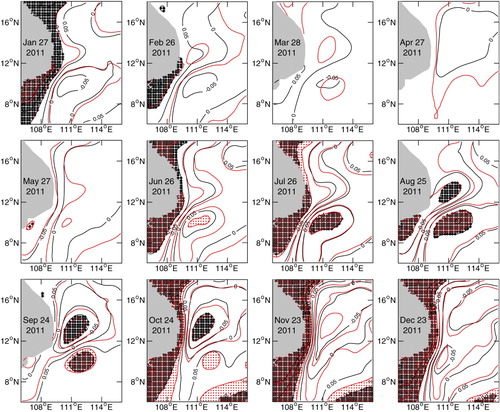
Fig. 12 Evolution of the observed SLA field (coloured shading) and the predicted SLA field with one-month lead time (contours) for 2011 (red lines are the zero contour line; solid black lines are negative contour lines; and dashed black lines are positive contour lines).

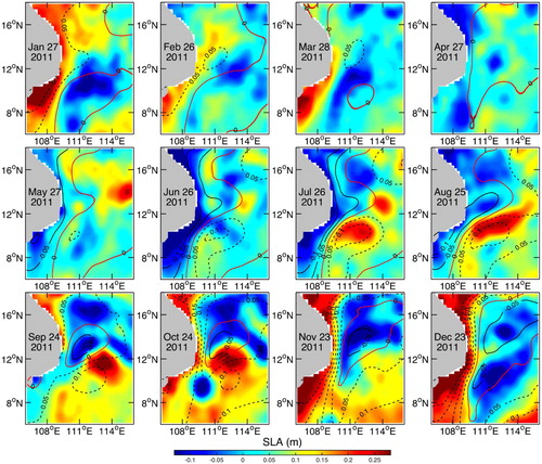
Fig. 13 (a) Forecast error estimate and (b) correlation coefficient of the predicted SLA field relative to the reconstructed SLA field (blue dots are the error for each forecast case, and the black line indicates the average of all 30 cases).

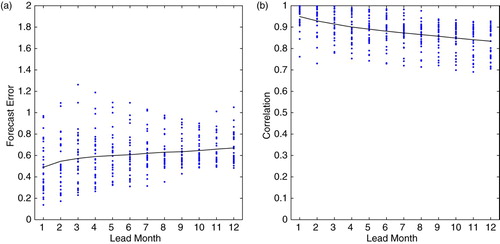
Fig. 14 (a) Forecast error estimate and (b) correlation coefficient of the predicted SLA field relative to the original SLA field (blue dots are the error for each forecast case, and the black line indicates the average of all 30 cases).

To further test the prediction capability of the SCS dipole structure, the predicted month that the dipole appears for each year is compared with the observed appearance in Table 2. If the predicted month is the same as the actual generation month, we mark that year with an R; otherwise, we mark it with a W. Because the training period data in the first several years is not sufficient to make an accurate prediction, we focus on the predictions from 1998 and later. With a one-month lead time in the prediction the accuracy of the forecast reaches 78%; when the lead time increases to 6 and 12 months, the forecast accuracy reduces to 72% and 61%, respectively. Finally, a prediction of the two-dimensional dipole structure in the following 12 months is plotted in Fig. 15. This prediction shows that the dipole structure in 2016 will appear in late August and disappear in late October.

Fig. 15 Predicted SLA field in the subsequent year with lead times varying from 1 to 12 months.

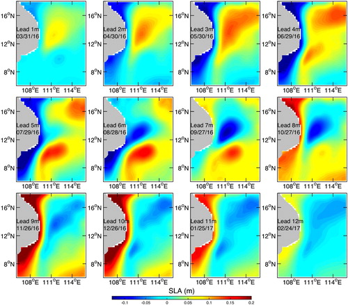
Table 2. Two-dimensional prediction of the SCS dipole structure.

Year	SLA Map	1-month Forecast	6-month Forecast	12-month Forecast
1998	none	R	R	W
1999	early July	W	R	W
2000	mid-August	R	W	W
2001	early August	R	R	W
2002	mid-July	W	W	R
2003	early August	R	R	R
2004	late July	R	R	R
2005	late June	R	W	R
2006	none	W	W	W
2007	none	R	R	W
2008	none	R	R	R
2009	early August	R	R	R
2010	none	R	R	W
2011	late August	R	W	R
2012	late July	R	R	R
2013	late August	W	R	R
2014	late July	R	R	R
2015	none	R	R	R
Accuracy		78%	72%	61%

4 Discussion

The SSA-MEM method is effective for any time series containing large oscillatory components. The deficiency of this method is that the forecast magnitudes of anomalies are usually weaker than observations. Mo (2001) used the SSA-MEM method to predict outgoing longwave radiation anomalies in the intraseasonal band over the Indian-Pacific sector and in the pan-American region. His results show that the average correlation between the predicted and observed anomalies is 0.65 at lead times of four pentads (20 days). Ghil and Jiang (1998) compared the six-month lead time SSA-MEM prediction with observations of Niño-3 SST anomalies, obtaining a correlation of 0.74. The lower prediction accuracy in those studies is caused by the weaker periodicity of the original time series. The dipole index is basically an annual oscillation and has much stronger periodicity, which makes the prediction more accurate.

Oceanic mesoscale eddies are the weather of the ocean and their prediction is a daunting challenge. However, the dipole structure in the SCS is a relatively stable type of mesoscale eddy that might lend itself to accurate prediction. With a statistical forecasting method, it is possible to make a useful prediction. Nevertheless, the SCS is a complicated dynamical system and the dipole can be influenced by many factors, such as wind, topography, ENSO, and the Kuroshio Intrusion (Qu et al., 2004). In order to test the utility of any prediction system, it will be more convincing to take a major influencing factor, such as wind, into consideration. Furthermore, the dipole is highly influenced by the state of ENSO. The dipole strength and the SCS summer monsoon are strong in the developing year of a warm ENSO event and weak or absent in the following decaying year. In strong El Niño years, the prediction is not as accurate as in normal years. The abnormal event strongly interferes with the prediction. To improve forecast accuracy, further studies need to be conducted to account for the dynamical effects of El Niño on the SCS dipole.

5 Conclusions

In this study, a dipole index is defined to monitor the generation, evolution, and termination of the SCS dipole. This index can characterize the dipole generation and termination time with a margin of error of two weeks. The index can also monitor the temporal evolution of the strength of the dipole. The SCS dipole structure typically appears in July, peaks in September, and disappears in November. The warm eddy component of the dipole often appears earlier than the cold eddy. After the generation of the dipole structure, the cold eddy propagates northeastward away from the coast, then after reaching its farthest east position, the cold eddy propagates back toward the coast and is absorbed by the wintertime southwestwardly flowing current along the coast of Vietnam. Because the upwelling and circulation variations associated with the dipole off the Vietnamese coast directly affect nutrient distribution and biomass productivity in the SCS, the prediction of the dipole's evolution is of considerable importance. Using a statistical forecasting method (SSA-MEM), a linear prediction of the dipole structure in both one and two dimensions is carried out. For a one-dimensional forecast, the average correlation coefficient between the predicted and observed dipole indices decreases from 0.99 with a one-month lead time to 0.81 with a one-year lead time. For the two-dimensional forecast, the forecast accuracy for the SCS dipole can reach 78% at one-month lead time and 61% at one-year lead time.

Acknowledgements

We acknowledge helpful advice from the reviewers. We are grateful for their support and contribution. The altimeter products used in this work are produced by SSALTO/DUACS and distributed by Aviso, with support from CNES (http://www.aviso.oceanobs.com/duacs).

Disclosure statement

No potential conflict of interest was reported by the authors.

Additional information

Funding

CD appreciates support from the National Key Research Program of China [grant number 2017YFA0604100], the Natural Science Foundation of China [grant number 41476022], and the National Programme on Global Change and Air–Sea Interaction [grant number GASI-IPOVAI-05].

References

- Bayler, E. J., & Liu, Z. (2008). Basin-scale wind-forced dynamics of the seasonal southern South China Sea gyre. Journal of Geophysical Research: Oceans, 113(C7), C07014. doi: 10.1029/2007JC004519
- Burg, J. P. (1968). A new analysis technique for time series data. Paper presented at Advanced Study Institute on signal Processing, NATO Enschede, Netherlands.
- Chen, C., & Wang, G. (2014). Interannual variability of the eastward current in the western South China Sea associated with the summer Asian monsoon. Journal of Geophysical Research C: Oceans, 119(9), 5745–5754. doi: 10.1002/2014JC010309
- Chen, D., & Yuan, X. (2004). A Markov model for seasonal forecast of Antarctic sea ice. Journal of Climate, 17(16), 3156–3168. doi: 10.1175/1520-0442(2004)017<3156:AMMFSF>2.0.CO;2
- Chen, G., Hou, Y., & Chu, X. (2011). Mesoscale eddies in the South China Sea: Mean properties, spatiotemporal variability, and impact on thermohaline structure. Journal of Geophysical Research: Oceans, 116(C6). doi:10.1029/2010JC006716 doi: 10.1029/98JC00366
- Chen, G., Hou, Y., Zhang, Q., & Chu, X. (2010). The eddy pair off eastern Vietnam: Interannual variability and impact on thermohaline structure. Continental Shelf Research, 30(7), 715–723. doi: 10.1016/j.csr.2009.11.013
- Chu, X., Xue, H., Qi, Y., Chen, G., Mao, Q., Wang, D., & Chai, F. (2014). An exceptional anticyclonic eddy in the South China Sea in 2010. Journal of Geophysical Research: Oceans, 119(2), 881–897.
- Dippner, J. W., Nguyen, K. V., Hein, H., Ohde, T., & Loick, N. (2007). Monsoon-induced upwelling off the Vietnamese coast. Ocean Dynamics, 57(1), 46–62. doi: 10.1007/s10236-006-0091-0
- Gan, J., & Qu, T. (2008). Coastal jet separation and associated flow variability in the southwest South China Sea. Deep Sea Research Part I: Oceanographic Research Papers, 55(1), 1–19. doi: 10.1016/j.dsr.2007.09.008
- Ghil, M., Allen, M. R., Dettinger, M. D., Ide, K., Kondrashov, D., Mann, M. E., … Yiou, P. (2002). Advanced spectral methods for climatic time series. Reviews of Geophysics, 40(1), 1003. doi: 10.1029/2000RG000092
- Ghil, M., & Jiang, N. (1998). Recent forecast skill for the El Niño/Southern Oscillation. Geophysical Research Letters, 25(2), 171–174. doi: 10.1029/97GL03635
- Keppenne, C. L. (1995). An ENSO signal in soybean futures prices. Journal of Climate, 8(6), 1685–1689. doi: 10.1175/1520-0442(1995)008<1685:AESISF>2.0.CO;2
- Kuo, N. J., Zheng, Q., & Ho, C.-R. (2000). Satellite observation of upwelling along the western coast of the South China Sea. Remote Sensing of Environment, 74(3), 463–470. doi: 10.1016/S0034-4257(00)00138-3
- Kuo, N. J., Zheng, Q., & Ho, C. R. (2004). Response of Vietnam coastal upwelling to the 1997–1998 ENSO event observed by multisensor data. Remote Sensing of Environment, 89(1), 106–115. doi: 10.1016/j.rse.2003.10.009
- Li, Y., Han, W., Wilkin, J. L., Zhang, W. G., Arango, H., Zavala-Garay, J., … Castruccio, F. S. (2014). Interannual variability of the surface summertime eastward jet in the South China Sea. Journal of Geophysical Research: Oceans, 119(10), 7205–7228. doi: 10.1002/2014JC010206
- Lian, T., & Chen, D. (2012). An evaluation of rotated EOF analysis and its application to tropical Pacific SST variability. Journal of Climate, 25(15), 5361–5373. doi: 10.1175/JCLI-D-11-00663.1
- Liu, Q., Jiang, X., Xie, S. P., & Liu, W. T. (2004). A gap in the Indo-Pacific warm pool over the South China Sea in boreal winter: Seasonal development and interannual variability. Journal of Geophysical Research: Oceans, 109(C7), C07012. doi: 10.1029/2003JC002179
- Mo, K. (2001). Adaptive filtering and prediction of intraseasonal oscillations. Monthly Weather Review, 129(4), 802–817. doi: 10.1175/1520-0493(2001)129<0802:AFAPOI>2.0.CO;2
- Penland, C., Ghil, M., & Weickmann, K. M. (1991). Adaptive filtering and maximum entropy spectra with application to changes in atmospheric angular momentum. Journal of Geophysical Research, 96(D12), 22659–22671. doi.org/10.1029/91JD02107
- Qu, T., Kim, Y. Y., Yaremchuk, M., Tuzuka, T., Ishida, A., & Yamagata, T. (2004). Can Luzon Strait transport play a role in conveying the impact of ENSO to the South China Sea? Journal of Climate, 17(18), 3644–3657. doi: 10.1175/1520-0442(2004)017<3644:CLSTPA>2.0.CO;2
- Tangang, F. T., Tang, B., Monahan, A. H., & Hsieh, W. W. (1998). Forecasting ENSO events: A neural network-extended EOF approach. Journal of Climate, 11(1), 29–41. doi: 10.1175/1520-0442(1998)011<0029:FEEANN>2.0.CO;2
- Wang, G., Chen, D., & Su, J. (2006). Generation and life cycle of the dipole in the South China Sea summer circulation. Journal of Geophysical Research: Oceans, 111(C6), C06002. doi: 10.1029/2005JC003314
- Wang, H. (2002). The instability of the East Asian summer monsoon–ENSO relations. Advances in Atmospheric Sciences, 19(1), 1–11. doi: 10.1007/s00376-002-0029-5
- Wu, Q., Yan, Y., & Chen, D. (2013). A linear Markov model for East Asian monsoon seasonal forecast. Journal of Climate, 26(14), 5183–5195. doi: 10.1175/JCLI-D-12-00408.1
- Xie, S. P., Chang, C. H., Xi, Q., & Wang, D. (2007). Intraseasonal variability in the summer South China Sea: Wind jet, cold filament, and recirculations. Journal of Geophysical Research: Oceans, 112(C10), C10008. doi: 10.1029/2007JC004238
- Xie, S. P., Xie, Q., Wang, D., & Liu, W. T. (2003). Summer upwelling in the South China Sea and its role in regional climate variations. Journal of Geophysical Research: Oceans, 118(C8), 3261. doi: 10.1029/2003JC001867
- Xue, Y., Leetmaa, A., & Ji, M. (2000). ENSO prediction with Markov models: The impact of sea level. Journal of Climate, 13(4), 849–871. doi: 10.1175/1520-0442(2000)013<0849:EPWMMT>2.0.CO;2