A Model Evaluation of Biological Effects on Seasonal Variation of Air–Sea CO₂ Flux in the Yellow and East China Seas

ABSTRACT

Based on a coupled physical-biogeochemical model of the Yellow and East China Seas (YECS), the influence of biological activity on the seasonal variation of the air–sea CO₂ flux is evaluated. The solution of a sensitivity experiment that excludes biological activity is compared with that of a reference experiment that includes the full processes. The comparison reveals that biological activity results in a much stronger seasonal variation of surface dissolved inorganic carbon (DIC) and, hence, the ratio of total alkalinity to DIC in the northern parts of the YECS. The increased ratio resulting from biological DIC consumption contributes to the undersaturated partial pressure of CO₂ at the sea surface with respect to the atmosphere, causing the central Yellow Sea in summer and autumn to shift from being a CO₂ source to a sink; this same shift also occurs over the Changjiang Bank in summer. In the southern YECS, the biological effect is relatively weak. The comparison further reveals that low water temperature, instead of biological activity, is the dominant factor causing the YECS to become a carbon sink in spring. The biological effect on the variation of DIC (both at the surface and in the water column) differs greatly among the three representative regions of the YECS because of differences in primary production and hydrodynamic conditions. Particle-tracking simulations quantify the regional difference in horizontal advection. In the northern region, weaker horizontal advection causes the longer residence time of low DIC water induced by biological consumption. Over the entire YECS, biological activity contributes to about one-third of the total annual absorption of atmospheric CO₂.

Résumé

[Traduit par la rédaction] Nous évaluons l’influence de l’activité biologique sur la variation saisonnière du flux air-mer du CO₂ à l’aide d’un modèle couplé physique-biogéochimique de la mer Jaune et de la mer de Chine orientale. Nous comparons la solution d’un test de sensibilité qui exclut l’activité biologique à celle d’un test de référence qui inclut le processus complet. La comparaison révèle que l’activité biologique entraîne une variation saisonnière forte du carbone inorganique dissous en surface et donc du rapport d’alcalinité totale sur le carbone inorganique dissous dans les portions nord de la région à l’étude. L’augmentation de ce rapport découlant de la consommation biologique du carbone inorganique dissous contribue à la pression partielle du CO₂ sous-saturé à la surface de la mer par rapport à l’atmosphère. Ce processus fait en sorte que la mer Jaune centrale, en été et en automne, devient un puits plutôt qu’une source de CO₂. Cette situation se produit aussi en été sur le banc du Changjiang. Dans le sud de la région marine à l’étude, l’effet biologique reste relativement faible. La comparaison révèle aussi que la faible température de l’eau, plutôt que l’activité biologique, est le facteur dominant transformant la région marine en puits de carbone au printemps. L’effet biologique sur la variation du carbone inorganique dissous (à la surface et dans la colonne d’eau) diffère grandement au sein des trois régions représentatives des mers Jaune et de Chine orientale, en raison des différences dans la production primaire et les conditions hydrodynamiques. Le suivi de particules simulées quantifie la différence régionale d’advection horizontale. Au nord, l’advection horizontale plus faible entraîne un temps de résidence accru de l’eau possédant un faible taux de carbone inorganique dissous, qu’a produit la consommation biologique. Sur toute la région des mers Jaune et de Chine orientale, l’activité biologique est responsable d’environ un tiers de l’absorption atmosphérique annuelle totale de CO₂.

KEYWORDS:

• air–sea CO₂ flux
• seasonal variation
• biological activity
• the Yellow and East China Seas

1 Introduction

A comprehensive understanding and quantifying of air–sea CO₂ exchange are key to the study of the global carbon budget and climate change (e.g., Benway & Doney, 2014). Presently, global coupled climate–carbon models, such as those assessed by the Intergovernmental Panel on Climate Change (IPCC), mainly evaluate carbon cycling in the open ocean, while large uncertainties remain in the role played by shelf waters (Dong et al., 2016; IPCC, 2014). Because of pronounced biological activity, the strong carbon fixation in shelf waters cannot be ignored in terms of the global air–sea CO₂ flux (ASCF). Variations of the ASCF in shelf seas, as well as the underlying mechanisms, need to be explored.

The ASCF is mainly determined by the partial pressure of CO₂ in the surface water (pCO_2w). The lower the value of pCO_2w, the better the ocean is at absorbing atmospheric CO₂. Previous studies concluded that oceanic carbon uptake is controlled by a complex interplay of chemical, biological, and hydrodynamic processes in seawater (e.g., Cai, Dai, & Wang, 2006; Heinze et al., 2015; Zhai & Dai, 2009). However, not all continental shelf seas respond in the same way to these processes (e.g., Arruda et al., 2015; Bates, 2006; Cahill, Wilkin, Fennel, Vandemark, & Friedrichs, 2016; Cossarini, Querin, & Solidoro, 2015; DeGrandpre, Olbu, Beatty, & Hammar, 2002; Fennel & Wilkin, 2009; Jiang, Cai, Wanninkhof, Wang, & Lüger, 2008; Signorini et al., 2013; Wåhlström, Omstedt, Björk, & Anderson, 2012; Xue et al., 2016). In some Arctic shelf waters, low pCO_2w is attributed to intense primary production during ice-free periods (e.g., Bates, 2006; Wåhlström et al., 2012). In the northern Adriatic Sea in the Mediterranean, an efficient carbon sink is attributed to a combination of high primary productivity and a strong continental shelf pump related to dense water formation (Cossarini et al., 2015). On the eastern shelf of the United States and in the North Sea, sea surface temperature (SST) and dissolved inorganic carbon (DIC) are the main factors that cause the seasonality of pCO_2w (e.g., Arruda et al., 2015; Fennel & Wilkin, 2009; Omar et al., 2010; Signorini et al., 2013). Still, on the eastern shelf of the United States, a recent model simulation highlighted the importance of water temperature in regulating the variability of the ACSF (e.g., Cahill et al., 2016). In the coastal waters off Georgia, United States, records from a moored autonomous pCO₂ system suggested that the annual cycle of pCO_2w is predominantly controlled by water temperature, while the influences of river input and biological processes are still substantial (e.g., Xue et al., 2016). Thus, we would expect each continental shelf system to have different carbon-cycling characteristics because of differences in relative contributions among the chemical, biological, and hydrodynamic processes.

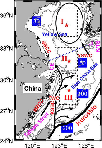
The Yellow and East China Seas (YECS), with a broad continental shelf shallower than 200 m, have a high level of primary production and are strongly affected by ocean circulation, including the intrusion of the Kuroshio Current, the Taiwan Warm Current (TWC), the Yellow Sea Warm Current (YSWC), and coastal currents (Fig. 1; e.g., Isobe, 2008; Lie & Cho, 2016; Su, 2001). As shown in Fig. 1, the Yellow Sea (YS) and the East China Sea (ECS) have a geographic boundary (blue dashed line) that connects the Changjiang estuary (CE) with Jeju Island (JI). The YS is a semi-enclosed shelf sea with a central trough in the north-south direction. In spring (March to May), phytoplankton blooms occur in the central YS as a result of rich nutrients supplied by strong vertical mixing and low turbidity that allows deeper penetration of light (e.g., Son, Campbell, Dowell, Yoo, & Noh, 2005; Zhou, Xuan, Huang, Liu, & Sun, 2013). In the shallower areas of the YS, primary production is light-limited because of high concentrations of suspended sediment (e.g., Son et al., 2005). In summer (June to August), the Yellow Sea Cold Water Mass with temperatures of approximately 7°C exists in the central YS beneath the warm water in the upper layer (Ho, Wang, Lei, & Xu, 1959). Primary production moves to a subsurface layer, with a relatively higher level along the tidal front (e.g., Wei et al., 2016). In autumn (September to November), phytoplankton blooms occur again in the surface water of the central YS when stratification is weakened, and nutrients can be replenished by vertical mixing (e.g., Son et al., 2005).

Fig. 1 Topography and schematic map of the circulation in the Yellow and East China Seas. The blue dotted line depicts the boundary between the Yellow Sea (YS) and the East China Sea (ECS). Solid black arrows denote the Yellow Sea Warm Current (YSWC), the Taiwan Warm Current (TWC), and branches of the Kuroshio Intrusion (including the Kuroshio Subsurface Branch Current (KSBC) carrying the Kuroshio Subsurface Water). Dotted curves with arrows at both ends indicate coastal currents whose directions change with the monsoon seasons (the Subei Coastal Current (SBCC) and the Min-Zhe Coastal Current (MZCC)). The closed oval outlines the Yellow Sea Cold Water Mass (YSCWM) that is present in summer. CE, JI, and K/TS denote the Changjiang Estuary, Jeju Island, and the Korea/Tsushima Strait, respectively. The dashed rectangular boxes define three representative regions: Region I for the central YS, Region II for the Changjiang Bank, and Region III for the middle shelf of the ECS. Red stars denote the positions of the vertical profiles shown in Fig. 5. Grey contours denote the 30, 50, 100, and 200 m isobaths, which will also be shown in Figs 3a, 4a, 6a, and 9.

Fresh water from the Changjiang River forms the Changjiang Diluted Water (CDW) and supplies a high level of nutrients. In the northern ECS, a year-round rich supply of nutrients is attributed to the CDW, which stimulates intense primary production in the nearshore region in summer (e.g., Gong, Wen, Wang, & Liu, 2003; Jiang et al., 2015; Ning, Shi, Cai, & Liu, 2004). In the southern ECS, after nutrients have been depleted by the spring bloom in the surface water, a subsurface chlorophyll a maximum develops over the middle and outer shelves in summer, fueled by rich nutrients from the Kuroshio Intrusion onto the shelf (Chen, 1996; Furuya, Hayashi, Yabushita, & Ishikawa, 2003; Guo, Zhu, Wu, & Huang, 2012). Therefore, the YECS are largely influenced by inputs (waters, nutrients, and carbon) from both the land and the deep ocean.

Observations have suggested that the shelf waters of the YECS annually act as carbon sinks, but uncertainties remain in terms of the seasonal and regional variations of carbon sinks and sources (e.g., Guo et al., 2015; Qu, Song, Yuan, Li, & Li, 2014, 2015; Qu et al., 2013; Tseng, Liu, Gong, Shen, & Cai, 2011; Tseng, Shen, & Liu, 2014; Zhai & Dai, 2009). In our previous study, a three-dimensional coupled physical-biogeochemical model was developed to simulate the spatial and seasonal changes in the ASCF in the YECS, and the factors influencing these changes were preliminarily analyzed (Luo, Wei, Liu, & Zhao, 2015). However, more in-depth analyses of the model results need to be carried out. For example, the model showed that both low water temperature and a phytoplankton bloom created favourable carbon-sink conditions in spring, but which factor is the main driver? Over the seasonal cycle, how do biological processes influence the surface inorganic carbon? Moreover, the net contribution of biological activity to the oceanic absorption of atmospheric CO₂ needs to be quantified. In this study, we attempt to answer these questions by conducting a model sensitivity experiment with the biological module turned off. The results of this experiment are compared with those of the reference experiment including the full processes. This method was used in a study of the North Sea (Lorkowski, Pätsch, Moll, & Kühn, 2012).

2 Model description

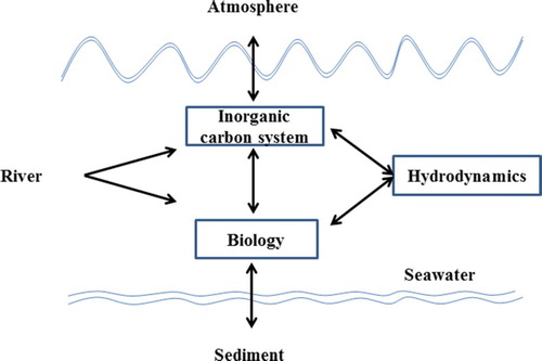
The three-dimensional coupled physical-biogeochemical model consists of three components: the hydrodynamic, biological, and inorganic carbon-cycling modules illustrated in a highly simplified format in Fig. 2. The hydrodynamic and biological modules are the same as those described by Zhao and Guo (2011). The carbon-cycling module was introduced in Luo et al. (2015). Some specific details of the model components are given below and in the appendix.

Fig. 2 Schematic illustration of the physical-biogeochemical model for the Yellow and East China Seas.

The hydrodynamic model is based on the Princeton Ocean Model (Blumberg & Mellor, 1987; Mellor, 1998), spanning a domain from approximately 24°N to 41°N and 117.5°E to 131.5°E (Fig. 1). The model has a horizontal resolution of 1/18° in longitude and latitude with 21 sigma levels in the vertical. It simulates temperature, salinity, ocean currents, sea surface height, and mixing due to turbulence. The model is driven by monthly climatology of surface atmospheric forcing; large-scale tidal and non-tidal currents at the lateral open boundaries; and runoff from major rivers along the coast. In particular, the model is forced with the surface wind stress climatology derived from Scatterometer Climatology of Ocean Winds. This climatology is based on eight years of daily satellite-based observations from Quick Scatterometer (Risien & Chelton, 2008). The model includes sea level changes due to the impacts of freshwater fluxes associated with precipitation minus evaporation and river runoff. Finally, the initial and open boundary conditions are interpolated from the simulations of the triple-nested models of Guo, Hukuda, Miyazawa, and Yamagata (2003).

The Nutrient-Phytoplankton-Zooplankton-Detritus biological module includes the following prognostic variables: three nutrients (nitrogen, phosphorus, and silicate), two phytoplankton functional types (diatoms and flagellates), and two types of detritus. In the main, biological activity includes photosynthesis, respiration, and mortality of phytoplankton; decomposition of detritus; and denitrification. The predation pressure from zooplankton for phytoplankton is parameterized in the death rate of algae. Evaluations of the seasonal cycles of nutrients and chlorophyll a can be found in Zhao and Guo (2011).

The inorganic carbon-cycling module contains the air–sea CO₂ exchange, riverine DIC input, interaction with the open ocean, and internal biological processes. In this module, DIC and total alkalinity (TA) are designed to be prognostic variables, while pCO_2w is a diagnostic variable that can be calculated based on DIC, TA, temperature, and salinity (Zeebe & Wolf-Gladrow, 2001). The chemical reactions when CO₂ dissolves in seawater are formulated according to Kantha (2004). The variation of carbon (C) associated with biological activity is related to nitrogen (N) according to the Redfield C:N ratio following models developed for waters off the east coast of the United States and the North Sea (e.g., Druon et al., 2010; Kühn et al., 2010). The initial conditions of DIC and TA, as well as the open boundary setting of DIC, are obtained from the seasonal climatology of the Carbon Dioxide Information Analysis Center (http://cdiac.ess-dive.lbl.gov/ftp/ndp076/; Goyet, Healy, & Ryan, 2000). This globally constructed dataset has a spatial resolution of 1° × 1° in longitude and latitude and 32 non-uniform layers in the vertical direction. An open-ocean relation of alkalinity versus salinity (Key et al., 2004) is used as an open boundary condition of TA. The particle organic carbon (POC) in the model is the summation of live phytoplankton and detritus. Because of the lack of detailed input data, the riverine POC flux is not considered. Our analysis focuses on the interior YECS where seasonal variations of carbon cycling are strongly influenced by hydrography and ocean circulation.

Based on the coupled physical-biogeochemical model described above, a reference simulation that includes the full processes was carried out. In this experiment, the hydrodynamic model was first run for 10 years and was then coupled to the biogeochemical component to run for three additional years. Model evaluation and analysis were applied to the results of the final year. Luo et al. (2015) described the evaluation of DIC distribution with observations. Subsequently Liu, Luo, Wei, and Zhao (2016) provided an evaluation of seasonal pCO_2w.

In our study, the solution of the reference simulation is compared with that of a sensitivity experiment. This new simulation is carried out using the same model as the reference simulation but with the biological module turned off. Consequently, inorganic carbon cycling in this sensitivity experiment is forced by the air–sea CO₂ exchange, hydrodynamic conditions, and the riverine DIC input. Because of the distinct spatial variation associated with the topographic features and hydrological structure, we divide the interior YECS into three typical sub-regions, namely the central YS (Region I), the Changjiang Bank (Region II), and the middle shelf of the ECS (Region III) (the dashed rectangular boxes in Fig. 1).

3 Influence of biology on DIC, pCO_2w, and carbon sinks and sources

a Distribution of chlorophyll a from reference experiment

Before analyzing the influence of biology on carbon cycling, we first describe the distribution of chlorophyll a obtained from the reference experiment. The main seasonal features of surface chlorophyll a concentration (Fig. 3a) is consistent with the in situ and satellite-based observations (e.g., Gong et al., 2003; Ning et al., 2004; Son et al., 2005). In Region I, a strong bloom occurs in spring and moves toward nearshore regions in summer. In autumn, the level of primary production in this region increases substantially. In Region II, a primary-production front appears near the coast in summer. In Region III, there is generally a substantially higher concentration of surface chlorophyll a in spring than in other seasons; however, the concentration is much lower than in Region I. Compared with observations, the model produces lower amounts of chlorophyll a in the western coastal area of the YECS. This underestimation is caused by the setting of a stronger limitation of light associated with high amounts of suspended sediments from the Changjiang River. This may bring a certain degree of uncertainty in carbon cycling near coastal areas. In this study, we focus on the interior of the YECS, leaving the simulation of coastal areas to be improved on in future studies.

Fig. 3 Chlorophyll a concentration from the reference experiment: (a) spatial distribution of seasonally averaged surface values (mg chl a m⁻³) and (b) monthly values (mg chl a m⁻²) obtained by vertical integration over the water column and horizontally averaging for the three representative regions.

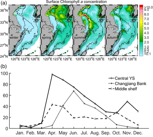
Figure 3b shows monthly values of chlorophyll a concentration obtained by vertically integrating over the water column and horizontally averaging for the three representative regions. In Region I, chlorophyll a concentration in the water column peaks in April, then gradually decreases until November. Very low productivity in the surface water and relatively high productivity in the water column in summer indicate the presence of subsurface chlorophyll a maxima. In Region II, primary production rises to a significant value in May, reaches a maximum in June, then decreases continuously until the end of the year. In Region III, chlorophyll a concentration shows similar high values in April, May, and October.

b Surface DIC

In the reference experiment, surface DIC exhibits a clear seasonal variation with higher values in cold seasons (winter (December to February) and spring) and lower values in warm seasons (summer and autumn) (see Fig. 3 in Luo et al., 2015). Without biological activity, the sensitivity experiment produces much weaker seasonal variations and generally higher values of surface DIC in all seasons (Fig. 4). In Region I, from April to December, excluding biological activity causes an increase in DIC concentration exceeding 50 μmol kg⁻¹, with the maximum increase being 100 μmol kg⁻¹ (Fig. 4b). In Region II, an increase of 30–50 μmol kg⁻¹ appears, mainly during summer, while a reduction of 0–50 μmol kg⁻¹ appears from late autumn to early spring (Fig. 4). In most areas to the south of Region II, the surface DIC concentration is similar to the reference experiment, except in the northern part of Region III (Fig. 4a).

Fig. 4 Comparison of surface DIC (μmol kg⁻¹) from the two experiments: (a) spatial distribution of seasonally averaged values (sensitivity minus reference) and (b) monthly values averaged over the three representative regions (solid lines for the reference simulation and dashed lines for the sensitivity simulation).

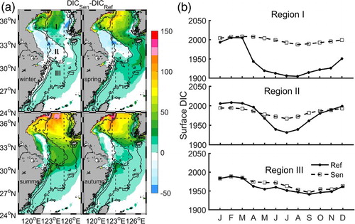
The significant influence of biological activity in Region I is attributed to the strong phytoplankton bloom that begins in April and gradually moves to coastal waters, following the availability of nutrients (Fig. 3) (Zhao & Guo, 2011). In Region II, the biological influence is evident mainly in summer, relating to a productivity front that occurs mainly during this season (Ning et al., 2004). In the sensitivity experiment, in Region II the reduction in surface DIC during the cold seasons is related to excluding the process of bio-detritus decomposition. This process has been recognized as a source of surface DIC based on observational studies (e.g., Chou, Gong, Cai, & Tseng, 2013). In most of the southern part of Region III, the influence of biological activity is weak.

The two experiments also show some common characteristics. In winter and early spring, surface DIC is higher than in the other seasons because of weak (or the absence of) biological consumption and strong vertical mixing. Meanwhile, lower water temperature enhances the solubility of atmospheric CO₂, in favour of maintaining the high surface DIC in the entire YECS. In Region II, the high DIC concentration in autumn is related to vertical mixing that brings bottom DIC-rich water to the surface (Luo et al., 2015). Clearly, physical processes (including the exchange of water masses and CO₂ solution) help to regulate surface DIC distribution but only cause a weaker seasonal cycle (Fig. 4b). In continental shelf seas with high primary production, the large seasonal changes in surface DIC are primarily caused by biological activity. Note that stable low DIC water exists in Region I from late spring to autumn in the reference experiment, despite decreasing chlorophyll a concentration after the spring bloom at the surface. This suggests that weak water exchange is at work to maintain the low DIC water.

c Vertical DIC in summer

Over the annual cycle, the largest influence of biological activity on surface DIC occurs in summer, at least in Regions I and II (Fig. 4). How does biological activity influence the vertical distribution of DIC in summer? Figure 5 shows the vertical profiles of DIC from the two simulations in August at three sites located near the centre of each representative region. The corresponding vertical profiles of water temperature and chlorophyll a concentration from the reference simulation are also presented.

Fig. 5 Vertical profiles of temperature (black curves; °C), chlorophyll a concentration (blue curves; mg chl a m⁻³), and DIC concentration (μmol kg⁻¹) obtained from the reference (solid red curves) and sensitivity (dashed red curves) experiments at three representative sites (red stars in Fig. 1) (a) Region I, (b) Region II, and (c) Region III.

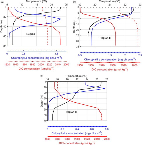
At the site in Region I, the two simulations show distinctly different vertical distributions of DIC (Fig. 5a). In the reference simulation, DIC concentration decreases from approximately 2045 μmol kg⁻¹ in the lower mixed layer to approximately 1920 μmol kg⁻¹ in the upper mixed layer. Without biological activity, DIC is nearly uniform with a concentration of approximately 2000–2015 μmol kg⁻¹. In the upper layer, the presence of biological consumption (as indicated by the chlorophyll a levels with a subsurface maximum) causes a reduction in DIC. In the lower layer, the reference simulation shows an increase in DIC compared with the sensitivity simulation because of the presence of biological decomposition. A relatively stable hydrodynamic condition in this region favours POC sinking; hence, there is significant remineralization in the lower layer with a very low level of primary production.

At the site in Region II, the vertical profiles of DIC from the two simulations have a similar shape, with the DIC concentration from the reference run being lower because of the biological consumption in the entire water column (Fig. 5b). The difference in DIC concentration between the two simulations decreases from the surface to the bottom, corresponding to the weakening of phytoplankton growth with increasing depth. The higher DIC in the lower layer compared with the upper layer in both simulations suggests that the intrusion of Kuroshio Subsurface Water, characterized by high DIC concentration, plays a role (Chen & Wang, 1999).

At the site in Region III, the vertical profiles of DIC from the two simulations are very similar, indicating that biological processes have a weak influence (Fig. 5c). This region is strongly influenced by the open ocean. Because of the strong currents associated with the intrusion of the Kuroshio, the water mass with properties changed by biological activity (creation of POC and reduction in DIC) is advected quickly out of this region. This results in weak (or nearly absent) decomposition of POC and, hence, nearly the same DIC concentration in the two experiments in the lower layer. Thus, vertical distribution of DIC in Region III is mainly controlled by that of the upstream water mass.

d Surface pCO_2w

Including biological activity, the reference experiment suggests that surface pCO_2w is overall higher in the southern region than in the northern region of the YECS year-round (Fig. 1 of Liu et al., 2016); the lowest pCO_2w of 200–270 µatm exists in Region I in spring; the highest pCO_2w of about 400 µatm is found in Region II during autumn and in Region III during summer (Fig. 6b). Excluding biological activity, the sensitivity experiment still obtains a clear seasonal cycle of surface pCO_2w (Fig. 6) with, however, generally higher values and some differences in seasonal distribution. The lowest pCO_2w values of 250–300 µatm are found in almost all of the YECS during winter, and the highest pCO_2w values are around 450–550 µatm in Region I during summer. This seasonal cycle of pCO_2w clearly follows that of SST (Fig. 6b), suggesting that without the biological effect the seasonality of pCO_2w is mainly regulated by the thermodynamic equilibrium processes. This situation is similar to that in the South China Sea where primary production is very low (Chai et al., 2009).

Fig. 6 (a) Spatial distribution of seasonally averaged pCO_2w (μatm) from the sensitivity experiment and (b) monthly values of SST (black curves; °C) and pCO_2w (μatm) from the reference (blue curves) and sensitivity (red curves) experiments, averaged over (a) Region I, (b) Region II, and (c) Region III.

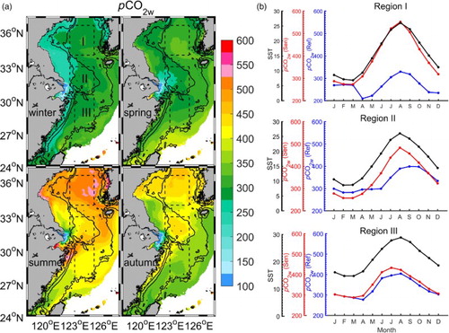
In the carbon component of our model, pCO_2w is estimated using water temperature, salinity, DIC, and TA (Kantha, 2004; Luo et al., 2015). Compared with the relatively weak influence of salinity, water temperature and the TA:DIC ratio influence the pCO_2w variation more strongly. Generally, pCO_2w increases with rising temperature and decreasing TA:DIC ratio (Chou, Gong, Sheu, Hung, & Tseng, 2009; Qu et al., 2015; Zeebe & Wolf-Gladrow, 2001). In the sensitivity experiment, SST determines the overall features of the seasonal variation of pCO_2w, while in the reference experiment the variation of pCO_2w is further influenced by the TA:DIC ratio. This ratio is primarily controlled by the DIC variation in the model. Without biological activity, DIC has a much higher concentration than that obtained from the reference experiment. Meanwhile, TA has similar values in the two experiments because of the minor role played by biological activity (diatoms and flagellates) in the TA variation. As a result, a lower TA:DIC ratio in the sensitivity experiment leads to a much higher pCO_2w (Fig. 6a) and, thus, weakens the capacity for the absorption of CO₂.

The regional and seasonal variations of pCO_2w are closely linked to whether each individual region of the YECS serves as a source or sink for atmospheric CO₂. This will be discussed in the following section.

e Carbon sink and/or source

The reference experiment suggests that, averaged over the annual cycle, the YECS serve as a carbon sink for atmospheric CO₂. The model estimated annual mean ASCF is −1.02 ± 0.5 mol C m⁻² yr⁻¹ in the YECS, with −0.94 ± 1.0 mol C m⁻² yr⁻¹ over the deeper parts of ECS shelf where water depth is greater than 30 m. Table 1 lists estimates of annual mean ASCF in the ECS based on observations, which are highly variable because of differences in sampling area and time. Our model estimate is within the range of the observed values, but detailed comparison is not further pursued here.

Table 1. Estimates of annual mean air–sea CO₂ flux in the ECS based on in situ observations. Negative values represent oceanic absorption of CO₂. The value after the ± sign denotes the standard deviation.

References	Air–Sea CO2 Flux (mol C m^−2 yr^−1)	Study Area
Tsunogai, Watanabe, & Sato (1999)	−2.9	PN^a line in the ECS (from 27.5°N, 128.4°E to 31.4°N, 123°E)
Zhang, Huang, Ma, Qiao, & Zhang (1997)	−3.76	ECS (25°–32°N, 121°–129°E)
Wang, Chen, Hong, & Chung (2000)	−1.2 to −2.8	Eastern ECS (28°–34°N, 124°–130°E)
Hu & Yang (2001)	−1.02	ECS
Song (2004)	−0.94	ECS
Shim et al. (2007)	−0.87	Northern ECS (31.5°–34°N, 124°–127.5°E)
Zhai & Dai (2009)	−1.93 ± 1.3	Northwestern ECS (30°–33°N, 122°–124°E)
Tseng et al. (2011)	−2.3 ± 0.4	ECS shelf (25°–32°N, 120°–128°E)
Qu et al. (2013)	−1.15	ECS shelf (25°–34°N, 120°–128°E)
Kim et al. (2013)	−2.2 ± 2.1	Northern ECS (31.5°–34°N, 124°–127.5°E)
Tseng et al. (2014)	−1.8 ± 0.5	ECS shelf (25°–32°N, 120°–128°E)
Guo et al. (2015)	−2.5 ± 1.5	ECS shelf (25°–33°N, 120°–128°E)

^aPN line, from (27°30′N, 128°15′E) to (30°30′N, 124°30′E) in the East China Sea.

Regarding the seasonal role played by the YECS in modulating atmospheric CO₂, it is very encouraging to find that our model results agree well with the general conclusion based on observations (e.g., Guo et al., 2015; Qu et al., 2013, 2014). In winter and spring the YECS overall serve as sinks for atmospheric CO₂. In summer, Regions I and II act as sinks, while Region III is a moderate source. In autumn, Region II is a significant source, while the remainder of the regions are carbon sinks (Luo et al., 2015). Annually, the entire YECS absorb 9.39 Tg C of atmospheric CO₂.

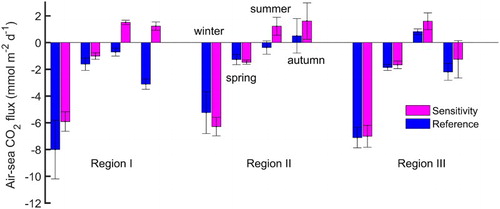
Excluding biological activity, the sensitivity experiment estimates an annual absorption of 6.16 Tg C of atmospheric CO₂ by the YECS, a 30% reduction from that estimated by the reference experiment. Figure 7 shows the seasonal ASCF averaged over the three regions from the two experiments. The differences identified are discussed below.

Fig. 7 Modelled air–sea CO₂ flux (mmol m⁻² d⁻¹) averaged over the three representative regions (defined by the rectangular boxes in Fig. 1). The mean and standard deviation of the flux in each region are represented by solid bars and vertical lines. The magenta and blue bars show the results from the sensitivity and reference experiments, respectively. In each region, four pairs of bars are presented for the four seasons (from left to right: winter, spring, summer, and autumn). Positive (negative) values represent oceanic emission (absorption) of CO₂.

1 REGION I: THE CENTRAL YS

In winter and spring, both simulations suggest that this area serves as a sink for atmospheric CO₂. By including biological effects, the reference experiment induces additional uptake in these two seasons relative to the sensitivity experiment. In summer and autumn, with biological activity included, this area acts as a sink for atmospheric CO₂; however, with no biological activity it acts as a source.

In the cold seasons of winter and spring, the ratio of TA to DIC in this region is generally larger than 1.10. When SST is less than 12°C, pCO_2w is generally undersaturated with respect to the atmosphere, regardless of the net biological effect (Figs 8a and 8c). Thus, relatively low SST is the primary reason for the region being a carbon sink. Biological effects further enhance oceanic CO₂ uptake. As to the variation of pCO_2w from winter to spring, differences in the TA:DIC ratio play a role when biological activity is included. According to the reference experiment, during this period, the TA:DIC ratio increases from 1.118 to 1.135, and the pCO_2w decreases from 258 µatm to 233 µatm (Fig. 8c). Without biological activity, DIC concentration and, hence, the TA:DIC ratio in the two seasons are similar; thus the small increase in pCO_2w from winter to spring is related to the increase in SST (Fig. 8c).

Fig. 8 Variations of pCO_2w (μatm, with axis being defined by dashed lines) as functions of SST (°C) and the TA:DIC ratio (assuming constant salinity values of 32 and 30 in Regions I and II, respectively). Panels (a) and (b) present all the seasonally averaged values in Regions I and II from the reference experiment. Panels (c) and (d) present the regionally averaged values in four seasons from the reference (stars connected by solid arrows) and sensitivity (squares) simulations. Blue, magenta, red, and black denote the values for winter, spring, summer, and autumn, respectively.

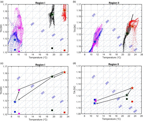
From spring to summer, the increasing TA:DIC ratio and SST have the opposite effects on the variation of pCO_2w, and their competition determines whether this area acts as a carbon sink or source. In both simulations, the same increase of 13°C in SST is a significant factor in the increase of pCO_2w. However, in the reference simulation, the increase of 0.025 in the TA:DIC ratio decelerates the SST-induced rise in pCO_2w, leading to undersaturated pCO_2w; hence, this region acts as a carbon sink. Without biological activity, pCO_2w is more than 500 µatm, leading to this region being a carbon source (Fig. 7). Therefore, the biological effects are the cause of Region I being a carbon sink in summer.

From summer to autumn, decreasing pCO_2w is caused by decreasing SST. But the undersaturated pCO_2w, hence the region being a carbon sink, is attributed to a relatively high TA:DIC ratio resulting from biological effects. Without biological activity, pCO_2w is oversaturated and the region becomes a carbon source (Fig. 7).

2 Region II: the Changjiang Bank

Compared with the results of the sensitivity experiment, including biological activity in the reference experiment causes a decrease in carbon absorption in this area during cold seasons. Similar to the situation in Region I, this area serves as a carbon sink (source) in summer with (without) biological activity. In autumn, biological effects reduce the CO₂ flux into the atmosphere relative to the sensitivity experiment.

Similar to the situation in Region I, pCO_2w is undersaturated with respect to the atmosphere when SST is less than 14°C, regardless of the net biological effect (Fig. 8b). Thus, low SST is the main cause of the region being a carbon sink in cold seasons. In the reference experiment, the substantially stronger decomposition of bio-detritus than growth of phytoplankton contributes to an increase in DIC concentration, thus slightly weakening the carbon sink (Fig. 7).

In summer, the significant influence of biological activity on the ASCF is a result of the high primary production that appears mainly in this season (Fig. 3; Ning et al., 2004). From spring to summer in the reference experiment, an increase in the TA:DIC ratio prevents a rapid rise in pCO_2w with increasing SST, resulting in a weak carbon sink. If biological drawdown of DIC becomes weaker, high SST tends to cause this area to be a carbon source, as suggested by the sensitivity experiment (Fig. 7).

In autumn, the biological effects can counteract the partial impacts of vertical mixing; however, it is not strong enough to replace vertical mixing as the dominant process causing Region II to be a carbon source (Luo et al., 2015). From summer to autumn, the increase in pCO_2w in the reference experiment is governed by the decrease in the TA:DIC ratio because of DIC supplementation through vertical mixing, while decreasing pCO_2w in the sensitivity experiment is governed by decreasing SST (Fig. 8d).

3 Region III: The middle shelf of the ECS

With and without biological activity, the two experiments obtain a similar seasonal variation of carbon sink and source. Differences in the ASCF between the two experiments suggest that biological activity has a negligible influence in winter and spring and causes an increase in CO₂ uptake in summer and autumn.

The chlorophyll a concentration in the water column on the middle shelf is comparable overall with that on the Changjiang Bank (Fig. 3); however, biological activity plays only a minor role in the surface DIC variation (Fig. 4) and vertical DIC distribution (Fig. 5c). In this region, DIC distribution is strongly influenced by the upstream water mass. In addition to this, the seasonal variation of pCO_2w is further regulated by that of SST and, thus, determines whether the region is a carbon sink or source.

4 Quantifying the differences in horizontal advection among the three regions

The comparison of results from the reference and sensitivity experiments in the previous section has revealed a more evident influence of biological activity on the variation of DIC and, thus, pCO_2w and the ASCF in the northern YECS than in the southern. This difference in biological effects is associated with that in hydrodynamic conditions in addition to phytoplankton growth.

In late spring, the formation of stratification blocks the supplementation of DIC-rich water from the lower layer to the surface layer. Thus, variation of DIC concentration at the surface is caused mainly by biological effects and horizontal exchange between different water masses. The strong horizontal current enhances the water exchange between local water and upstream water. The weak horizontal current tends to limit water exchange and helps maintain the low DIC water induced by biological consumption for a period of time in the original area. The residual low DIC water continually influences pCO_2w. This process is similar to the concept of the durative effect of biological DIC drawdown proposed by Zhai et al. (2014). To quantify the horizontal advection in the three representative regions, we carried out particle-tracking simulations using the model-simulated currents.

Taking the central YS as an example, phytoplankton growth begins in April and extends vertically to the layer at 20–30 m depth from spring to autumn. Thus, the passive particles released at each model grid at the surface and at 30 m depth are tracked for five months from 1 April to 31 August based on the daily-averaged horizontal currents. The time step for tracking is one hour. At the end of each month, the remaining particles in the region are counted. The proportion of remaining particles relative to the total number of released particles in a region is used as an index for the effect of horizonal advection on DIC exchange. That is, a larger (smaller) proportion corresponds to a weaker (stronger) advection effect. The above procedure was carried out for each of the three representative regions.

a Region I: The central YS

The particles released at both the surface and at 30 m depth drift southeastward and enter the Korea Strait (Fig. 9). Until the end of June, the proportions of particles remaining in this region at the surface and 30 m depth are 55% and 68%, respectively (Table 2). The remaining water is characterized by low DIC because of the spring phytoplankton bloom and helps to create a high TA:DIC ratio, hence, the undersaturation of pCO_2w in summer.

Fig. 9 Positions of particles at the end of April, May, and June (left to right) after being released on 1 April at each model grid in each region. Upper (a)–(c) and lower (d)–(f) panels are for particles released at the surface and at 30 m depth, respectively. Blue, red, and black denote particles released in Regions I, II, and III, respectively.

Table 2. Statistics derived from the particle-tracking simulations. The particles were released on 1 April in three regions at the surface and at 30 m depth. The percentage values denote the proportion of particles remaining relative to the total number of particles released in each region on the five dates indicated.

	Region I: Central YS		Regioin II: Changjiang Bank		Region III: Middle shelf of ECS
	Surface (%)	30 m Depth (%)	Surface (%)	30 m Depth (%)	Surface (%)	30 m Depth (%)
30 April	71	83	59	39	42	6
31 May	67	74	60	18	5	0
30 June	55	68	23	7	2	0
31 July	34	62	1	2	0	0
31 August	30	60	1	0	0	0

At the beginning of autumn (i.e., 31 August), 30% of the total particles released on 1 April stay at the surface, while 60% remain at 30 m depth (Table 2). This suggests weaker horizontal advection in the lower layer. Water exchange occurs between Region I and the coastal area at the surface. This process also contributes to a low DIC concentration in Region I because the coastal water has a low DIC concentration induced by high primary production in summer. The subsurface chlorophyll a maximum in summer creates the relatively low DIC water, which remains under the surface layer of Region I. This subsurface residual water restrains the rapid increase in surface DIC in autumn despite the enhanced wind-induced upper-water mixing. Thus, DIC concentration remains steady and low from late spring to autumn in the central YS.

b Region II: The Changjiang Bank

At the surface, 23% of the total number of particles released remain in this region after three months of tracking, and nearly all (99%) of the particles depart this area by late July (Table 2). At 30 m depth, only 18% of the total number of particles released remain after two months of tracking (31 May). Compared with Region I, Region II experiences stronger advection, hence, a shorter residence time for water with biological DIC drawdown.

c Region III: The middle shelf of the ECS

This region is significantly affected by open-ocean currents (Su, 2001). Particles released at the surface and at 30 m depth move toward the Tsushima Strait following the strong current (Fig. 9). After a month, 42% of the total number of particles released at the surface remain in this region, while only 6% remain at 30 m depth (Table 2). This suggests very strong advection over the middle shelf. Hence, the photosynthesis-induced low DIC water moves out of the region quickly, weakening the biological effect.

Overall, horizontal advection decreases from Region III to I. In addition to differences in primary production, weak horizontal advection increases the influence of biological activity on carbon cycling in the northern area of the YECS compared with the southern area.

5 Conclusions and discussion

In this study, the influence of biological activity on the carbon system in the YECS is evaluated by analyzing the results of a coupled physical-biogeochemical model. The solution of the reference experiment that includes the full processes is compared with that of the sensitivity experiment without the biology component. This reveals that biological processes contribute to a much stronger seasonal variation of surface DIC, hence the ratio of TA to DIC, significantly influencing the variation of pCO_2w in the northern parts of the study area. Including biological processes, the shift from being a carbon source to a carbon sink occurs in the central YS in summer and autumn and over the Changjiang Bank in summer. In the southern parts of the study area, the biological effect is relatively weak. The comparison further clarifies that low SST is the dominant cause of the YECS being a carbon sink in spring, despite the presence of a phytoplankton bloom.

The influence of biological activity on carbon cycling is associated with primary production and hydrodynamic conditions. Weaker (stronger) horizontal circulation tends to limit (enhance) DIC exchange between different water masses. Low DIC water induced by biological consumption can be maintained for a period of time in the original region with weak advection, which continually influences pCO_2w. Particle-tracking simulations using modelled horizontal currents suggest that the advection effect decreases from the middle shelf, to the Changjiang Bank, to the central YS. Consequently, the biological effect is more evident in the northern than in the southern areas of the YECS.

Overall, model results suggest that biological processes contribute to about one-third of the total annual absorption of atmospheric CO₂ by the entire YECS (estimated to be 9.39 Tg C yr⁻¹). This indicates the benefits of maintaining a healthy marine ecosystem to decelerate the increase in atmospheric CO₂. However, shelf water is not the eventual destination of the absorbed atmosphere CO₂. The biologically fixed carbon, mainly in the form of new primary production, will be buried in the sediment layer of the continental shelf or transported into the deep ocean for slower cycling. Thus, more complete carbon budget analyses for the YECS, including the ACSF, POC production, POC sedimentation, and DIC and POC exchanges with the deep ocean need to be considered in future studies.

Toward quantifying the contribution of continental shelf seas to the global carbon budget, it is of great interest to examine the similarities and differences of different regions. Here, we compare the carbon cycling in the YECS with that in the North Sea over the northwestern European continental shelf. Both regions feature a wide continental shelf and have been identified as areas where a continental shelf pump affects the transfer of carbon from the shelf to the open ocean (Thomas, Bozec, Elkalay, & de Baar, 2004; Tsunogai et al., 1999).

The North Sea is a two-part system with distinct biogeochemistry (e.g., Kühn et al., 2010; Emeis et al., 2015; Clargo, Salt, Thomas, & de Baar, 2015). The southern North Sea (SNS) is shallow (with depths less than 50 m) and well mixed. This region is similar to most of the coastal areas of the YECS, except Region II. Although shallower than 50 m, stratification is evident in Region II due to the influence of CDW and surface heating. Riverine input of nutrients fuels a high level of primary production making Region II a weak carbon sink in summer, while conditions in the SNS cause it to be a carbon source. The northern North Sea (NNS) exhibits seasonal stratification and acts as a carbon sink all year round. The NNS is influenced by North Atlantic water with a relatively low level of DIC concentration. After passing through the North Sea, Atlantic water is enriched by approximately 40 μmol kg⁻¹ of additional DIC (Bozec, Thomas, Elkalay, & de Baar, 2005). Similarly, Region III of the YECS is connected to the northwest Pacific and influenced by Kuroshio Subsurface Water. However, Kuroshio Subsurface Water has a higher DIC concentration than the shelf water (Chen & Wang, 1999). In addition, the two regions display different summer SSTs: Region III is above 25°C, but the NNS is below 20°C. The model study of Lorkowski et al. (2012) suggested that increasing SST can cause declining oceanic uptake of atmospheric CO₂ in the North Sea. The differences in DIC input from the open ocean and local SST result in the different roles played by the two regions in regulating atmospheric CO₂ in summer: the NNS being a carbon sink while Region III is a carbon source. The similarities and differences between the YECS and the North Sea, in terms of their seasonal and regional variations, play a role in regulating atmospheric CO₂, and this suggests the need for regional studies to quantify the contribution of shelf seas to the global carbon budget.

Acknowledgements

We thank Professor Moto Ikeda and three anonymous reviewers for constructive comments on the original manuscript.

Disclosure statement

No potential conflict of interest was reported by the authors.

Additional information

Funding

This study was supported by the National Key Research and Development Program of China [grant number 2016YFC1401602] and the National Natural Science Foundation of China [grant number 41630969] and [grant number 41376112]. Liang Zhao was funded by the National Key Research and Development Program of China [grant number 2016YFA0601301] and [grant number 2016YFC1401602] and the Strategic Priority Research Program of the Chinese Academy of Sciences [grant number XDA11020305].

Appendix

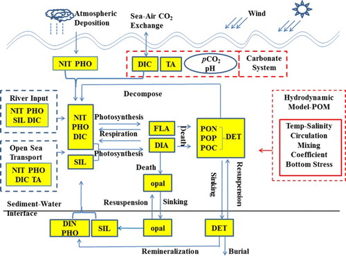
In this section, we provide some details of the biogeochemical model. Figure A1 shows a comprehensive schematic overview. In the inorganic carbon system module DIC and TA are designated as prognostic variables, and pCO_2w in the water is a diagnostic variable. The governing equations for DIC and TA in seawater are(A1) (A2) where adv, diff, B, F, and RIV denote advection, diffusion, biological processes, air–sea CO₂ exchange, and river input terms, respectively, and t is the time.

The variation of DIC associated with biological activity is expressed with a Redfield C:N ratio for variation of dissolved inorganic nitrogen (NIT) due to photosynthesis, respiration, and decomposition. The governing equation of NIT is(A3) here R, D, P, RIVD, and denote the respiration, decomposition, photosynthesis, river and atmospheric deposition (fluxes), and source and sink terms due to sedimentation and resuspension, respectively; DIA, FLA, and DET are prognostic variables in the biological module, corresponding to diatom, flagellates, and detritus. Skogen and Soiland (1998) provided a summary of equations in the biological module. TA increases by one mole corresponding to the uptake of one mole of NIT by phytoplankton under consumption. Remineralization of phytodetritus has the reverse effect on TA (Zeebe & Wolf-Gladrow, 2001).

depends on the difference in pCO₂ between surface water () and the atmosphere (), the solubility of CO₂ in seawater () (Weiss, 1974), and CO₂ transfer velocities () (Wanninkhof, 1992). The relevant equations are(A4) (A5) (A6) where is a function of the air pressure (P), saturation vapour pressure of water () (Weiss & Price, 1980), and molar fraction of CO₂ in dry air () (Zeebe & Wolf-Gladrow, 2001). Sea surface pCO_2w is calculated according to SST, sea surface salinity (SSS), DIC, and TA through a series of chemical processes between CO₂ and water (see details in Kantha, 2004). The process of air–sea CO₂ exchange does not change TA.

The initial conditions for DIC and TA, as well as the open boundary setting of DIC, were obtained from the seasonal dataset of the Carbon Dioxide Information Analysis Center (http://cdiac.ess-dive.lbl.gov/ftp/ndp076/; Goyet et al., 2000). Global monthly molar fraction of CO₂ in dry air with a horizontal resolution of 3° × 2° in longitude and latitude, for the period 2000 to 2001, were downloaded from the website of the U.S. National Oceanic and Atmospheric Administration (ftp://aftp.cmdl.noaa.gov/products/carbontracker/co2/molefractions/). The monthly climatology of surface wind and air pressure, with 1/4° in longitude and latitude for the period 1989 to 2009, were obtained from the European Centre for Medium-range Weather Forecasts-Reanalysis DATA Archive-Interim (ECMWF-ERA; http://apps.ecmwf.int/datasets/data/interim-full-daily/levtype = sfc/). At the river–sea interface, the annual input of DIC from the Changjiang River is assigned to different months corresponding to the monthly variation of runoff. In the open ocean, TA is mainly controlled by salinity (Millero, Lee, & Roche, 1998); therefore, the open boundary condition for TA is set to TA = 65.8881S – 4.124 (Key et al., 2004), where S is salinity.

Fig. A1 Schematic overview of the biogeochemical model for the Yellow and East China Seas. Prognostic variables are shown in yellow boxes.

References

- Arruda, R., Calil, P. H., Bianchi, A. A., Doney, S. C., Gruber, N., Lima, I., & Turi, G. (2015). Air-sea CO2 fluxes and the controls on ocean surface pCO2 seasonal variability in the coastal and open-ocean southwestern Atlantic Ocean: A modeling study. Biogeosciences (online), 12(19), 5793–5809. doi: 10.5194/bg-12-5793-2015
- Bates, N. R. (2006). Air-sea CO2 fluxes and the continental shelf pump of carbon in the Chukchi Sea adjacent to the Arctic Ocean. Journal of Geophysical Research, 111, C10013. doi: 10.1029/2005JC003083
- Benway, H. M., & Doney, S. C. (2014). Scientific outcomes and future challenges of the Ocean Carbon and biogeochemistry program. Oceanography, 27(1), 106–107. doi: 10.5670/oceanog.2014.13
- Blumberg, A. F., & G. L. Mellor. (1987). A description of a three-dimensional coastal ocean circulation model. In N. Heaps (Ed.), Three-dimensional coastal ocean models, Coastal and Estuarine Series, No. 4 (pp. 1–16). Washington, DC: Am. Geophys. Union.
- Bozec, Y., Thomas, H., Elkalay, K., & de Baar, H. J. (2005). The continental shelf pump for CO2 in the North Sea—evidence from summer observation. Marine Chemistry, 93(2), 131–147. doi: 10.1016/j.marchem.2004.07.006
- Cahill, B., Wilkin, J., Fennel, K., Vandemark, D., & Friedrichs, M. (2016). Inter-annual and seasonal variability in air-sea CO2 fluxes along the US Eastern continental shelf and their sensitivity to increasing air temperatures and variable winds. Journal of Geophysical Research: Biogeosciences, 121, 295–311. doi: 10.1002/2015JG002939
- Cai, W. J., Dai, M. H., & Wang, Y. C. (2006). Air-sea exchange of carbon dioxide in ocean margins: A province-based synthesis. Geophysical Research Letters, 33, L12603. doi: 10.1029/2006GL026219
- Chai, F., Liu, G. M., Xue, H. J., Shi, L., Chao, Y., Tseng, C. M., … Liu, K. K. (2009). Seasonal and interannual variability of carbon cycle in South China Sea: A three-dimensional physical-biogeochemical modeling study. Journal of Oceanography, 65, 703–720. doi: 10.1007/s10872-009-0061-5
- Chen, C. T. A. (1996). The Kuroshio intermediate water is the major source of nutrients on the East China Sea continental shelf. Oceanoligica Acta, 19 (5), 523–527.
- Chen, C. T. A., & Wang, S. L. (1999). Carbon, alkalinity and nutrient budgets on the East China Sea continental shelf. Journal of Geophysical Research: Oceans, 104(C9), 20675–20686. doi: 10.1029/1999JC900055
- Chou, W. C., Gong, G. C., Cai, W. J., & Tseng, C. M. (2013). Seasonality of CO2 in coastal oceans altered by increasing anthropogenic nutrient delivery from large rivers: Evidence from the Changjiang-East China Sea system. Biogeosciences (online), 10(6), 3889–3899. doi: 10.5194/bg-10-3889-2013
- Chou, W. C., Gong, G. C., Sheu, D. D., Hung, C. C., & Tseng, T. F. (2009). Surface distribution of carbon chemistry parameters in the East China Sea in summer 2007. Journal of Geophysical Research: Oceans, 114, C07026. doi: 10.1029/2008JC005128
- Clargo, N. M., Salt, L. A., Thomas, H., & de Baar, H. J. (2015). Rapid increase of observed DIC and pCO2 in the surface waters of the North Sea in the 2001–2011 decade ascribed to climate change superimposed by biological processes. Marine Chemistry, 177, 566–581. doi: 10.1016/j.marchem.2015.08.010
- Cossarini, G., Querin, S., & Solidoro, C. (2015). The continental shelf carbon pump in the northern Adriatic Sea (Mediterranean Sea): Influence of wintertime variability. Ecological Modelling, 314, 118–134. doi: 10.1016/j.ecolmodel.2015.07.024
- DeGrandpre, M. D., Olbu, G. J., Beatty, C. M., & Hammar, T. R. (2002). Air-sea CO2 fluxes on the US Middle Atlantic Bight. Deep Sea Research Part II: Topical Studies in Oceanography, 49, 4355–4367. doi: 10.1016/S0967-0645(02)00122-4
- Dong, F., Li, Y. C., Wang, B., Huang, W. Y., Shi, Y. Y., & Dong, W. H. (2016). Global air-sea CO2 flux in 22 CMIP5 models: Multiyear mean and interannual variability. Journal of Climate, 29(7), 2407–2431. doi: 10.1175/JCLI-D-14-00788.1
- Druon, J. N., Mannino, A., Signorini, S., McClain, C., Friedrichs, M., Wilkin, J., & Fennel, K. (2010). Modeling the dynamics and export of dissolved organic matter in the northeastern U.S. continental shelf. Estuarine, Coastal and Shelf Science, 88(4), 488–507. doi: 10.1016/j.ecss.2010.05.010
- Emeis, K. C., van Beusekom, J., Callies, U., Ebinghaus, R., Kannen, A., Kraus, G., … Möllmann, C. (2015). The North Sea—A shelf sea in the Anthropocene. Journal of Marine Systems, 141, 18–33. doi: 10.1016/j.jmarsys.2014.03.012
- Fennel, K., & Wilkin, J. (2009). Quantifying biological carbon export for the northwest North Atlantic continental shelves. Geophysical Research Letters, 36, L18605. doi: 10.1029/2009GL039818
- Furuya, K., Hayashi, M., Yabushita, Y., & Ishikawa, A. (2003). Phytoplankton dynamics in the East China Sea in spring and summer as revealed by HPLC-derived pigment signatures. Deep Sea Research Part II: Topical Studies in Oceanography, 50, 367–387. doi: 10.1016/S0967-0645(02)00460-5
- Gong, G. C., Wen, Y. H., Wang, B. W., & Liu, G. J. (2003). Seasonal variation of chlorophyll a concentration, primary production and environmental conditions in the subtropical East China Sea. Deep Sea Research Part II: Topical Studies in Oceanography, 50, 1219-1236. doi: 10.1016/S0967-0645(03)00019-5
- Goyet, C., Healy, R. J., & Ryan, J. P. (2000). Global distribution of total inorganic carbon and total alkalinity below the deepest winter mixed layer depths. ORNL/CDIAC-127, NDP-076. Oak Ridge, Tennessee: Carbon Dioxide Information Analysis Center, Oak Ridge National Laboratory, U.S. Department of Energy. doi: 10.3334/CDIAC/otg.ndp076
- Guo, X. H., Zhai, W. D., Dai, M. H., Zhang, C., Bai, Y., Xu, Y., … Wang, G. Z. (2015). Air-sea CO2 fluxes in the East China Sea based on multiple-year underway observations. Biogeosciences (online), 12(18), 5495–5514. doi: 10.5194/bg-12-5495-2015
- Guo, X. Y., Hukuda, H., Miyazawa, Y., & Yamagata, T. (2003). A triply nested ocean model for simulating the Kuroshio—Roles of horizontal resolution on JEBAR. Journal of Physical Oceanography, 33, 146–169. doi: 10.1175/1520-0485(2003)033<0146:ATNOMF>2.0.CO;2
- Guo, X. Y., Zhu, X. H., Wu, Q. S., & Huang, D. J. (2012). The Kuroshio nutrient stream and its temporal variation in the East China Sea. Journal of Geophysical Research: Oceans, 117, C01026. doi: 10.1029/2011JC007292
- Heinze, C., Meyer, S., Goris, N., Anderson, L., Steinfeldt, R., Chang, N., … Bakker, D. C. E. (2015). The ocean carbon sink – Impacts, vulnerabilities and challenges. Earth System Dynamics, 6, 327–358. doi: 10.5194/esd-6-327-2015
- Ho, C. B., Wang, Y. X., Lei, Z. Y., & Xu, S. (1959). A preliminary study of the formation of Yellow Sea cold mass and its properties. Oceano. Et Limno. Sini., 1, 11–15. [in Chinese, with English abstract].
- Hu, D. X., & Yang, Z. S. (2001). Key processes of marine fluxes in the East China Sea. Beijing: China Ocean Press. [in Chinese].
- IPCC. (2014). Climate change 2014: Synthesis report. Contribution of Working Groups I, II and III to the Fifth Assessment Report of the Intergovernmental Panel on Climate Change. [Edited by Core Writing Team, R. K. Pachauri, and L. A. Meyer]. Geneva: Author.
- Isobe, A. (2008). Recent advances in ocean-circulation research on the Yellow Sea and East China Sea shelves. Journal of Oceanography, 64, 569–584. doi: 10.1007/s10872-008-0048-7
- Jiang, L. Q., Cai, W. J., Wanninkhof, R., Wang, Y., & Lüger, H. (2008). Air-sea CO2 fluxes on the U.S. South Atlantic Bight: Spatial and seasonal variability. Journal of Geophysical Research: Oceans, 113, C07019. doi: 10.1029/2007JC004366
- Jiang, Z. B., Chen, J. F., Zhou, F., Shou, L., Chen, Q. Z., Tao, B. Y., … Wang, K. (2015). Controlling factors of summer phytoplankton community in the Changjiang (Yangtze River) Estuary and adjacent East China Sea shelf. Continental Shelf Research, 101, 71–84. doi: 10.1016/j.csr.2015.04.009
- Kantha, L. H. (2004). A general ecosystem model for applications to primary productivity and carbon cycle studies in the global oceans. Ocean Modelling, 6, 285–334. doi: 10.1016/S1463-5003(03)00022-2
- Key, R., Kozyr, A., Sabine, C., Lee, K., Wanninkhof, R., Bullister, J., … Peng, T. H. (2004). A global ocean carbon climatology: Results from Global Data Analysis Project (GLODAP). Global Biogeochemical Cycles, 18, GB4031. doi: 10.1029/2004GB002247
- Kim, D., Choi, S. H., Shim, J., Kim, K. H., & Kim, C. H. (2013). Revisiting the seasonal variations of sea-air CO2 fluxes in the northern East China Sea. Terrestrial, Atmospheric and Oceanic Sciences, 24, 409–419. doi: 10.3319/TAO.2012.12.06.01
- Kühn, W., Pätsch, J., Thomas, H., Borges, A. V., Schiettecatte, L. S., Bozec, Y., & Prowe, A. F. (2010). Nitrogen and carbon cycling in the North Sea and exchange with the North Atlantic—A model study, Part II: Carbon budget and fluxes. Continental Shelf Research, 30(16), 1701–1716. doi: 10.1016/j.csr.2010.07.001
- Lie, H. J., & Cho, C. H. (2016). Seasonal circulation patterns of the Yellow and East China Seas derived from satellite-tracked drifter trajectories and hydrographic observations. Progress in Oceanography, 146, 121–141. doi: 10.1016/j.pocean.2016.06.004
- Liu, Z., Luo, X. F., Wei, H., & Zhao, L. (2016). Influence of increasing nutrients of the Changjiang River on air–sea CO2 flux in adjacent seas. Journal of Tianjin University of Science and Technology, 31, 55–63. doi: 10.133641j.issn.1672-6510.20150270 [in Chinese, with English Abstract]
- Lorkowski, I., Pätsch, J., Moll, A., & Kühn, W. (2012). Interannual variability of carbon fluxes in the North Sea from 1970 to 2006–Competing effects of abiotic and biotic drivers on the gas-exchange of CO2. Estuarine, Coastal and Shelf Science, 100, 38–57. doi: 10.1016/j.ecss.2011.11.037
- Luo, X. F., Wei, H., Liu, Z., & Zhao, L. (2015). Seasonal variability of air–sea CO2 fluxes in the Yellow and East China Seas: A case study of continental shelf sea carbon cycle model. Continental Shelf Research, 107, 69–78. doi: 10.1016/j.csr.2015.07.009
- Mellor, G. L. (1998). Users guide for a three dimensional, primitive equation, numerical ocean model. Princeton, NJ: Program in Atmospheric and Oceanic Sciences, Princeton University. Retrieved from https://www.researchgate.net/publication/242777179
- Millero, F. J., Lee, K., & Roche, M. (1998). Distribution of alkalinity in the surface waters of the major oceans. Marine Chemistry, 60(1), 111–130. doi: 10.1016/S0304-4203(97)00084-4
- Ning, X. R., Shi, J. X., Cai, Y. M., & Liu, C. G. (2004). Biological productivity front in the Changjiang Estuary and the Hangzhou Bay and its ecological effects. Acta Oceanologia Sinica, 26, 96–106. [in Chinese, with English Abstract].
- Omar, A. M., Olsen, A., Johannessen, T., Hoppema, M., Thomas, H., & Borges, A. V. (2010). Spatiotemporal variations of fCO2 in the North Sea. Ocean Science, 6(1), 77–89. doi: 10.5194/os-6-77-2010
- Qu, B. X., Song, J. M., Yuan, H. M., Li, X. G., & Li, N. (2014). Air-sea CO2 exchange process in the southern Yellow Sea in April of 2011, and June, July, October of 2012. Continental Shelf Research, 80, 8–19. doi: 10.1016/j.csr.2014.02.001
- Qu, B. X., Song, J. M., Yuan, H. M., Li, X. G., & Li, N. (2015). Summer carbonate chemistry dynamics in the Southern Yellow Sea and the East China Sea: Regional variations and controls. Continental Shelf Research, 111, 250–261. doi: 10.1016/j.csr.2015.08.017
- Qu, B. X., Song, J. M., Yuan, H. M., Li, X. G., Li, N., Duan, L. Q., … Chen, X. (2013). Advances of seasonal variations and controlling factors of the sea-air CO2 flux in the East China Sea. Advances in Earth Science, 28, 783–793. [in Chinese, with English Abstract]
- Risien, C. M., & Chelton, D. B. (2008). A global climatology of surface wind and wind stress fields from eight years of QuikSCAT Scatterometer data. Journal of Physical Oceanography, 38, 2379–2413. doi: 10.1175/2008JPO3881.1
- Shim, J. H., Kim, D., Kang, Y. C., Lee, J. H., Jang, S. T., & Kim, C. H. (2007). Seasonal variations in pCO2 and its controlling factors in surface seawater of the northern East China Sea. Continental Shelf Research, 27, 2623–2636. doi: 10.1016/j.csr.2007.07.005
- Signorini, S. R., Mannino, A., Najjar, R. G. Jr., Friedrichs, M. A. M., Cai, W. J., Salisbury, J., … Shadwick, E. (2013). Surface ocean pCO2 seasonality and sea-air CO2 flux estimates for the North American east coast. Journal of Geophysical Research: Oceans, 118, 5439–5460. doi: 10.1002/jgrc.20369
- Skogen, M. D., & Soiland, H. (1998). A user’s guide to NORWECOM V2.0. The Norwegian ecological model system. Bergen-Nordnes: Institue of Marine Research, Division of Marine Environment. Retrieved from https://core.ac.uk/download/pdf/30846984.pdf
- Son, S. H., Campbell, J., Dowell, M., Yoo, S. J., & Noh, J. (2005). Primary production in the Yellow Sea determined by ocean color remote sensing. Marine Ecology Progress Series, 303, 91–103. doi: 10.3354/meps303091
- Song, J. M. (2004). Biogeochemistry of China Seas. Jinan: Shandong Science & Technology Press. [in Chinese].
- Su, J. L. (2001). A review of circulation dynamics of the coastal oceans near China. Acta Oceanologica Sinica, 23, 1–16. [in Chinese, with English Abstract].
- Thomas, H., Bozec, Y., Elkalay, K., & de Baar, H. J. (2004). Enhanced open ocean storage of CO2 from shelf sea pumping. Science, 304(5673), 1005–1008. doi: 10.1126/science.1095491
- Tseng, C. M., Liu, K. K., Gong, G. C., Shen, P. Y., & Cai, W. J. (2011). CO2 uptake in the East China Sea relying on Changjiang runoff is prone to change. Geophysical Research Letters, 38, L24609. doi: 10.1029/2011GL049774
- Tseng, C. M., Shen, P. Y., & Liu, K. K. (2014). Synthesis of observed air–sea CO2 exchange fluxes in the river-dominated East China Sea and improved estimates of annual and seasonal net mean fluxes. Biogeosciences (online), 11(14), 3855–3870. doi: 10.5194/bg-11-3855-2014
- Tsunogai, S., Watanabe, S., & Sato, T. (1999). Is there a “continental shelf pump” for the absorption of atmospheric CO2? Tellus B: Chemical and Physical Meteorology, 51, 701–712. doi:10.1034/j.1600-0889.1999.t01-2-00010.x
- Wang, S. L., Chen, C. T. A., Hong, G. H., & Chung, C. S. (2000). Carbon dioxide and related parameters in the East China Sea. Continental Shelf Research, 20(4), 525–544. doi: 10.1016/S0278-4343(99)00084-9
- Wanninkhof, R. (1992). Relationship between wind speed and gas exchange over the ocean. Journal of Geophysical Research, 97, 7373–7382. doi: 10.1029/92JC00188
- Wåhlström, I., Omstedt, A., Björk, G., & Anderson, L. G. (2012). Modelling the CO2 dynamics in the Laptev Sea, Arctic Ocean: Part I. Journal of Marine Systems, 102-104, 29–38. doi: 10.1016/j.jmarsys.2012.05.001
- Wei, Q. S., Li, X. S., Wang, B. D., Fu, M. Z., Ge, R. F., & Yu, Z. G. (2016). Seasonally chemical hydrology and ecological responses in frontal zone of the Central Southern Yellow Sea. Journal of Sea Research, 112, 1–12. doi: 10.1016/j.seares.2016.02.004
- Weiss, R. F. (1974). Carbon dioxide in water and seawater: The solubility of a non-ideal gas. Marine Chemistry, 2, 203–215. doi: 10.1016/0304-4203(74)90015-2
- Weiss, R. F., & Price, B. A. (1980). Nitrous oxide solubility in water and seawater. Marine Chemistry, 8, 347–359. doi: 10.1016/0304-4203(80)90024-9
- Xue, L., Cai, W. J., Hu, X., Sabine, C., Jones, S., Sutton, A. J., … Reimer, J. J. (2016). Sea surface carbon dioxide at the Georgia time series site (2006–2007): Air–sea flux and controlling processes. Progress in Oceanography, 140, 14–26. doi: 10.1016/j.pocean.2015.09.008
- Zeebe, R. E., & Wolf-Gladrow, D. (2001). CO2 in seawater: Equilibrium, kinetics, isotopes. Amsterdam: Elsevier Oceanography Series 65.
- Zhai, W. D., Chen, J. F., Jin, H. Y., Li, H. L., Liu, J. W., He, X. Q., & Bai, Y. (2014). Spring carbonate chemistry dynamics of surface waters in the northern East China Sea: Water mixing, biological uptake of CO2, and chemical buffering capacity. Journal of Geophysical Research: Oceans, 119, 5638–5653. doi: 10.1002/2014JC009856
- Zhai, W. D., & Dai, M. H. (2009). On the seasonal variation of air–sea CO2 fluxes in the outer Changjiang (Yangtze River) Estuary, East China Sea. Marine Chemistry, 117, 2–10. doi: 10.1016/j.marchem.2009.02.008
- Zhang, Y. H., Huang, Z. Q., Ma, L. M., Qiao, R., & Zhang, B. (1997). Carbon dioxide in surface water and its flux in East China Sea. Journal of Oceanography Taiwan Strait, 16, 374. [in Chinese, English Abstract].
- Zhao, L., & Guo, X. Y. (2011). Influence of cross-shelf water transport on nutrients and phytoplankton in the East China Sea: A model study. Ocean Science, 7, 27–43. doi: 10.5194/os-7-27-2011
- Zhou, F., Xuan, J. L., Huang, D. J., Liu, C. G., & Sun, J. (2013). The timing and the magnitude of spring phytoplankton blooms and their relationship with physical forcing in the central Yellow Sea in 2009. Deep Sea Research Part II: Topical Studies in Oceanography, 97, 4–15. doi: 10.1016/j.dsr2.2013.05.001