Stochastic Post-Processing of CFSR Daily Precipitation across Canada

ABSTRACT

Reanalyses, based on numerical weather prediction methods assimilating past observations, provide continuous precipitation datasets and represent interesting options for assessing the climatology of regions with sparse station networks (e.g., northern Canada). However, reanalysis series cannot be used directly because of possible biases and mismatch between their spatial and temporal resolutions with that needed for local applications. To address these issues, a Stochastic Model Output Statistics (SMOS) approach was selected to post-process precipitation series simulated by the Climate Forecast System Reanalysis (CFSR) across Canada. This approach uses CFSR precipitation as a covariate and is based on two regression models: the first one is a logistic regression that deals with precipitation occurrence, and the second is a vector generalized linear model for precipitation intensity. At-site post-processed daily precipitation series are randomly generated using the SMOS approach, and selected climate indicators from the Expert Team on Climate Change Detection and Indices, which is jointly sponsored by the Commission for Climatology of the World Meteorological Organization's (WMO) World Climate Data and Monitoring Programme, the Climate Variability and Predictability Programme of the World Climate Research Programme, and the Joint WMO-IOC Technical Commission for Oceanography and Marine Meteorology (CCI/CLIVAR/JCOMM) are estimated and compared with corresponding observed and CFSR values. The two models in the SMOS approach, in addition to adequately correcting systematic biases, produced better predictions than the climatology of the wet and dry and intensity sequences. Additionally, the SMOS generally yields consistent climate indices when compared with those from CFSR without post-processing, though there is still room for improvement for specific indices (e.g., annual maximum of cumulative wet days).

RÉSUMÉ

[Traduit par la rédaction] Les réanalyses, fondées sur des méthodes de prévision numérique du temps qui assimilent les observations existantes, fournissent des champs continus de données de précipitations et représentent une option intéressante pour évaluer la climatologie des régions où les stations de mesures restent rares (p. ex., le nord du Canada). Cependant, nous ne pouvons utiliser directement les données de réanalyses en raison de biais éventuels et d’incompatibilité entre leurs résolutions spatiale et temporelle et celles qui conviennent aux applications locales. Pour résoudre ces problèmes, nous avons choisi des statistiques de sortie de modèles stochastiques (SMOS), afin de traiter a posteriori les précipitations simulées par le système de réanalyse Climate Forecast System Reanalysis (CFSR), pour l’ensemble du Canada. Cette méthode utilise les précipitations de la CFSR comme covariable et s’appuie sur deux modèles de régression. Le premier est une régression logistique qui analyse l’occurrence des précipitations et le second est un modèle vectoriel généralisé de régression linéaire de l’intensité des précipitations. Des séries de données de précipitations quotidiennes sont générées aléatoirement aux sites, et ce, à l’aide de la méthode SMOS et d’indicateurs de climat provenant de l’Équipe d’experts pour la détection et la surveillance des changements climatiques et les indices de changements climatiques, que financent conjointement la Commission de climatologie de l’Organisation météorologique mondiale (OMM) dans le cadre du Programme mondial de recherche sur le climat, le projet de variabilité et prévisibilité du climat du Programme mondial de recherche sur le climat, et la Commission technique mixte OMM/COI d’océanographie et de météorologie maritime, puis elles sont estimées et comparées avec les données correspondantes, observées et issues de la CFSR. Les deux modèles de la méthode des SMOS, en plus de corriger adéquatement les biais systématiques, produisent de meilleures prévisions que la climatologie des jours pluvieux et secs, et de l’intensité des précipitations. De plus, les SMOS produisent généralement des indices climatologiques cohérents par rapport à ceux des CFSR sans post-traitement, bien que certains indices restent ā améliorer (p. ex. le nombre maximal annuel de jours pluvieux).

KEYWORDS:

• reanalysis
• daily precipitation
• precipitation modelling
• stochastic post-processing

1 Introduction

Precipitation records are essential for urban infrastructure design, power production, and flood control (Devine & Mekis, 2008). Accurate rainfall datasets over long periods of time, from dense station networks, are necessary for several applications, such as the design of urban infrastructures based on Intensity-Duration-Frequency curves (CSA, 2012) or agricultural impact assessments (Ambrosino, Chandler, & Todd, 2014). The earliest available precipitation records across Canada date back to the 1870s (Metcalfe, Routledge, & Devine, 1997) and cover relatively short periods of time with limited and uneven spatial coverage. The need to access alternative daily precipitation datasets extending the coverage of the current network is particularly important in Canada, especially in northern regions that are expected to be developed in the near future (Allard & Lemay, 2012).

Among the newly available datasets, reanalyses represent an attractive alternative for assessing the historical climate of poorly monitored regions. Reanalysis reconstructs the past state of the atmosphere using numerical weather prediction models that assimilate past observations, generating spatially and temporally continuous meteorological fields that are also consistent (Bengtsson & Shukla, 1988). Several reanalysis datasets have been developed in recent years. They differ, in their assimilation techniques, atmospheric models, spatial and temporal resolutions, and the time periods covered as well as other aspects. Reanalysis products are not only extensively used to drive Regional Climate Models (RCMs) for reference periods but are also increasingly employed to directly assess historical climate and weather series (Bosilovich, Chen, Robertson, & Adler, 2008; Donat et al., 2014; Zhang, Kornich, & Holmgren, 2013, among others). Many studies have used precipitation datasets from reanalyses over different climatic regions (e.g., southern Africa; Zhang et al., 2013), at different time scales (e.g., seasonal mean; Higgins, Kousky, Silva, Becker, & Xie, 2010), and to investigate different characteristics (e.g., analysis of extremes; Donat et al., 2014). This literature review highlights the dependence of reanalysis performance on the selected characteristics (e.g., annual maximum), the statistics (e.g., mean over a given period), the regions, the period, and the temporal scale. Comparisons of various reanalyses over different regions (Bromwich, Nicolas, & Monaghan, 2011; Eum, Dibike, Prowse, & Bonsal, 2014; Rusticucci, Zazulie, & Raga, 2014, among others) have not demonstrated that one particular reanalysis is systematically better than any of the others.

Precipitation reanalysis may need to be post-processed before it can be used (e.g., as input data for hydrological models or impact studies). The post-processing of the precipitation reanalysis aims to correct possible bias and scale mismatch (representativeness error; Tustison, Harris, & Foufoula-Georgiou, 2001) between the grid cells and at-site precipitation. Several approaches dealing with the scale discrepancy between the global or regional climate model (GCM or RCM) and the local-scale variables, also known as downscaling methods, have been proposed in the literature. These methods can be physically (Fowler, Blenkinsop, & Tebaldi, 2007) or statistically based (see Maraun et al. (2010), for an extensive review of these approaches). The post-processing used in this study is based on statistical tools that belong to the Stochastic Model Output Statistics family of methods (SMOS; Maraun et al., 2010; Wong et al., 2014). The SMOS enables local-scale time series generation by explicitly modelling the local-scale variability of precipitation through a statistical link (usually regression models) between large-scale and its local-scale weather observations (Maraun, 2013). This approach, therefore, differs from deterministic Model Output Statistics approaches in which biases are “removed” through a correction function relating simulated and observed variables that do not account for any noise unexplained by the predictors (e.g., quantile mapping; Piani, Haerter, & Coppola, 2010). The current research also showed similarities with the fields of the statistical modelling of precipitation (Wilks & Wilby, 1999) but differed by the conditioning physical variable. In fact, the statistical modelling of precipitation generally uses several reanalysis synoptic covariates (exogenous to the precipitation) that drive the precipitation process such as sea level pressure (SLP), geopotential height, or specific humidity (Lavers, Prudhomme, & Hannah, 2013).

The objective of this paper is to investigate how stochastic post-processing, based on reanalysis daily precipitation series, may be used to estimate at-site climate indicators (e.g., annual maximum of wet spell durations). This study is a first step in the development of a post-processing method whose objective is to take advantage of the post-processed information provided by the reanalysis to stochastically generate precipitation series at ungauged sites. The SMOS approach was, therefore, first applied at sites where observations were available to check the performance consistency of this approach across a large domain with contrasting climatic regions. Further work will consider more advanced models to improve, for instance, the representation of the spatiotemporal structure (Ben Alaya, Ouarda, & Chebana, 2018; Serinaldi & Kilsby, 2014). The goal is to generate various historical statistics at sites with short or incomplete records or at ungauged sites. This is a particularly important issue in Canada, where the station network density is very low, especially in northern regions. The Climate Forecast System Reanalysis (CFSR; Saha et al., 2010) was considered. The relative performance of post-processed and CFSR precipitation series in terms of estimated annual and seasonal climate indicators was also investigated. The selected approach enabled correction and downscaling of daily CFSR precipitation. However, other climate characteristics at different time scales, such as annual duration of wet spells, were not explicitly corrected by the post-processing approach and were, therefore, not evaluated at calibration sites. Comparison with CFSR datasets is relevant because CFSR could display good performance for climatic indicators at annual or seasonal time scales. The selected post-processing approach proceeds in two steps; the first one deals with precipitation occurrence and the second with precipitation intensity on the day with precipitation.

Few studies using stochastic approaches to downscale reanalysis-driven GCM/RCM precipitation have been carried out (Eden, Widmann, Maraun, & Vrac, 2014; Wong et al., 2014), and, to our knowledge, only Eum, Cannon, and Murdock (2017) have directly used reanalysis precipitation for downscaling purposes. Wong et al. (2014) used this methodology to post-process reanalysis-driven RCMs for nine stations across the United Kingdom. The authors also explicitly modelled precipitation extremes through a mixture of gamma and generalized Pareto distributions. The authors demonstrated the ability of this approach to correct systematic bias and to provide good estimates of local precipitation distributions for a wide range of quantiles. Very high quantiles were better represented by the mixed distribution but were computationally expensive. Eden et al. (2014) used a similar approach to assess the added value of post-processed RCMs relative to post-processed GCMs. They showed that, according to some skill scores, downscaled precipitation using a GCM as a predictor outperformed the one using an RCM as a predictor. The differences in the atmospheric modelling in the GCM and the RCM were mentioned by these authors as a possible explanation for these counterintuitive findings. Vaittinada Ayar et al. (2016) reached a similar conclusion after applying six statistical downscaling methods, including SMOS, to reanalysis-driven GCM precipitation and five reanalysis-driven RCMs. Across Canada, Asong, Khaliq, and Wheater (2016a) used a multi-site generalized linear model (GLM) framework to simulate daily precipitation series and temperature over the Prairie Provinces by using large-scale variables from the National Centers for Environmental Prediction/National Center for Atmospheric Research (NCEP/NCAR) Reanalysis I (Kalnay et al., 1996). However, their aim was not to post-process reanalysis precipitation, as in the current study, but to simulate local-scale daily precipitation distributions from large-scale weather variables (e.g., relative humidity) (perfect prog method; Maraun et al., 2010). They also applied the multi-site GLM model parameters to regrid large-scale covariates from the Earth System Model (ESM) in order to evaluate climate change impact on daily precipitation and temperature (Asong, Khaliq, & Wheater, 2016b). The two novel contributions by this paper were, first, to only use precipitation from the reanalysis as a covariate, which results in a simple approach that can be readily implemented, and second, to investigate a much larger geographic region encompassing a range of diverse climates.

The paper is structured as follows. Available datasets are presented in Section 2, while the stochastic post-processing framework is described in Section 3. Section 4 presents the evaluation approach and results are summarized in Section 5. Finally, the conclusions are given in Section 6.

2 Study domain and datasets

Daily-observed precipitation series at 4881 stations were initially considered, 463 of which belong to the second generation Adjusted Precipitation for Canada dataset (APC2; Environment and Climate Change Canada, 2013; Mekis & Vincent, 2011). The APC2 series were adjusted to account for wind undercatch, evaporation, funnel wetting with regards to rain, and improved snow density assessment (Devine & Mekis, 2008; Mekis & Vincent, 2011). The remaining stations were provided by Environment and Climate Change Canada and the Ministère du Développement Durable, de l’Environnement et de la Lutte contre les Changements Climatiques (MDDELCC) of Quebec. For this study, station records were preferred to interpolated datasets because interpolation errors in gridded products based on sparse station networks can be high, especially for extremes and climate indices (e.g., Contractor, Alexander, Donat, & Herold, 2015; Gervais, Tremblay, Gyakum, & Atallah, 2014; Hofstra, New, & McSweeney, 2010; Way, Oliva, & Viau, 2017).

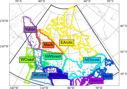
Quality control of the observed series required the following criteria: (i) each year was required to have less than 10% missing daily values to be considered a valid year; (ii) stations were required to have at least 10 valid years within the study period (1979–2009) with more than five consecutive valid years. This last criterion was imposed to keep the short-length northern stations in the studied network and to avoid datasets that were excessively sparse at the annual scale. Further quality control steps, presented in the Appendix, were also applied. A total of 1884 valid precipitation series were identified and considered further for analysis. Figure 1 presents the spatial distribution of the selected stations and the climate regions as defined by Plummer et al. (2006).

Fig. 1 Rainfall network used and the CFSR domain (thick black frame). Climatic regions are: Yukon (Yukon), Mackenzie (Mack), East Arctic (EArctic), West Coast (WCoast), Western Cordillera (WCrdra), North Western Forest (NWforest), Northern Plains (NrnPlains), North East Forest (NEforest), Great Lakes (GLakes) and Maritimes (Marit) (Plummer et al., 2006).

The CFSR was produced by NCEP with the Coupled Forecast System (CFS) model and covers the 1979–2009 period (Saha et al., 2010). This model simulates the past state of the ocean and atmosphere at a horizontal resolution of 0.312° latitude × 0.312° longitude (∼25 km at 45°N), by assimilating quality-controlled observations. The CFSR differs from other reanalyses in that it uses a coupled atmosphere–ocean–sea-ice–land model (Bromwich et al., 2011) and assimilates satellite radiances during the entire period; it also includes the time evolution of CO₂ concentrations (for more details see Mesinger et al., 2006). In the land model, CFSR also includes two gridded precipitation products and (i) the Climate Prediction Center (CPC) unified global daily gauge analysis and (ii) the pentad dataset of the CPC Merged Analysis of Precipitaion (CMAP) (Saha et al., 2010, and references therein). The CFSR hourly precipitation amounts were aggregated to daily values over a domain covering Canada (Fig. 1). The CFSR precipitation was selected in this study as a preliminary analysis (not shown for conciseness) and showed that CFSR precipitation provides overall good representation of the spatial distribution and precipitation amounts when compared with observations. Moreover, despite biases in the intensities, on a daily basis the temporal correspondence, necessary for probabilistic regression models, between the observed and the corresponding CFSR daily precipitation series was generally good.

3 Stochastic post-processing of daily precipitation

Stochastic post-processing includes defining precipitation occurrence and intensity for a given day in terms of conditional probability distribution given CFSR precipitation intensity for the same day at the corresponding grid cell. The main goal is to provide local precipitation intensity distributions for each day, conditional on CFSR precipitation for the same day, before creating multiple possible time series by randomly sampling these distributions (Maraun et al., 2015). Post-processing of CFSR precipitation, therefore, proceeded in two steps (Chandler & Wheater, 2002; Coe & Stern, 1982; Wong et al., 2014): post-processing was first applied to precipitation occurrence and second to precipitation intensity for “wet” days. Post-processing was achieved independently on each CFSR grid cell with at least one corresponding station. The CFSR precipitation was compared with each station series independently when more than one station was included in a CFSR grid cell (around 35% of the grid cells).

Daily precipitation series were modelled with mixed discrete and continuous distributions to account for, respectively, the occurrence of dry and wet days and precipitation intensity on wet days (Neykov, Neytchev, & Zucchini, 2014). In the following, a “wet” day is defined as a day with more than 1 mm of precipitation (Dai, 2006; Schmidli, Frei, & Vidale, 2006; Sun, Solomon, Dai, & Portmann, 2006, among others). Such a threshold value is necessary, because reanalysis, as well as regional and global climate models, too frequently simulate low intensity precipitation (see, e.g., Sun et al., 2006).

a Post-processing of precipitation occurrence

The conditional probability of the occurrence of precipitation, , at a given station on a given day was estimated using a logistic regression (LR; Buishand, Shabalova, & Brandsma, 2004; Wong et al., 2014). The LR is a linear regression model in which the predictand is binary and the predictor may be binary or continuous (Stern & Coe, 1984). In the present study, the predictand of the LR model is the wet or dry condition of day , one or zero, respectively, as recorded at the station. The log-transformed (Chandler, 2002) daily CFSR precipitation was used as a predictor, and to account for possible seasonality in the post-processing of occurrence probabilities, sine and cosine correction terms were also considered. The conditional probability, , that day is wet was, therefore, defined as(1) where is the logit function, is the Julian day, days is the average yearly period for cosine and sine waves accounting for leap years, and are the regression coefficients estimated by maximum likelihood (MLE).

b Post-Processing of Precipitation Intensity

The gamma distribution was selected to model daily precipitation intensity (Katz, 1977; Wilks, 2011, among others). Preliminary analysis demonstrated the overall good fit of the gamma distribution to the observed precipitation intensity. However, the light tail of the gamma distribution led to underestimations of the very high quantiles at specific sites (Katz, 1977; Vrac & Naveau, 2007). Shape () and mean () parameters were considered (McCullag & Nelder, 1989), and the scale parameter is, therefore, given by and the variance by . The probability density function is given by(2) where is the gamma function and the daily precipitation intensity.

The daily local precipitation intensity distribution, conditional on CFSR precipitation, was defined within the vector generalized linear model (VGLM) framework (Yee & Wild, 1996). Parameters and of the gamma distribution on day were expressed as a function of the log-transformed CFSR daily intensity (). Seasonal post-processing terms were also considered for the mean . The resulting expressions are(3) where is the log link function, days, and and are the regression coefficients estimated using MLE with the VGAM package in the R environment (Yee, 2016). As the 1 mm threshold defining wet days () led to misfits of the small intensities, all precipitation on wet days were shifted by −1 mm before estimating parameter values and then shifted back by +1 mm (Wong et al., 2014). Model selection is discussed in Section 5.

Combining the conditional probability of occurrence (Eq. (1)) and the cumulative distribution function (CDF) of the daily precipitation intensity (CDF from Eqs (2) and (3)), the CDF of the local precipitation intensity on day , , can be written as(4) In the following, will be written as to simplify notation.

4 Evaluation of the post-processing models

a Predictive Power of Regression Models

In order to evaluate the predictive power of the LR and VGLM models, two forecast skill scores were considered (Wilks, 2011). Skill scores compare forecasts from a given model to a reference, here the climatological forecast (Friederichs & Thorarinsdottir, 2012). Their values range from −∞ to 1, with negative values indicating a forecast skill worse than climatology, a zero value indicating a forecast skill similar to climatology, and a value of one indicating a perfect forecast.

The Brier Skill Score (BSS) was used to evaluate the LR model. The Brier Score (BS; Wilks, 2011) assesses the synchronicity of observed dry and wet days ( or , for the dry or wet condition, respectively, at day ) with the LR-estimated conditional probability of occurrence (, ranging from 0 to 1) (Wong et al., 2014):(5) Here denotes the total number of days in the time series. The BSS, was computed to compare the performance of the LR model to a climatological forecast (i.e., the probability of precipitation occurrence from observations over the studied period). A BSS value larger than zero, therefore, indicates that post-processed reanalysis provides a “better” forecast than the one based on the probability of occurrence of dry and wet days.

The Continuous Rank Probability Skill Score (CRPSS) was used to assess the skill of the VGLM model. The Continuous Rank Probability Score (CRPS, Hersbach, 2000) provides an overall evaluation of the predictive skill of a model forecast by comparing the forecast distribution () with the empirical CDF of daily recorded intensities () (Bentzien & Friederichs, 2014; Friederichs & Thorarinsdottir, 2012):(6) where corresponds to the Heaviside function with the step at the observed precipitation intensity on day and being the sample size. Reference CRPS used for the skill score estimates (CRPSS) compared the CDF of the fitted gamma distribution without covariates to .

Annual and seasonal skill scores were evaluated to identify possible seasonal differences in model predictive power. In the following, the year is split into winter (December, January, and February: DJF), spring (March, April, and May: MAM), summer (June, July, and August: JJA), and autumn (September, October, and November: SON). In the seasonal case, reference forecasts were assessed for each season; for instance, a gamma distribution without covariates was fitted over the SON months for the studied period.

b Evaluation of Annual Precipitation Index Series

In addition to the aforementioned model evaluation, the post-processing approach was also investigated in terms of its ability to reproduce annual precipitation index series. Annual and seasonal precipitation indices, selected from the joint Commission for Climatology (CCL) of the World Meteorological Organization's World Climate Data and Monitoring Programme, the Climate Variability and Predictability (CLIVAR) Programme of the World Climate Research Programme, and the Joint WMO-IOC Technical Commission for Oceanography and Marine Meteorology (JCOMM) Expert Team (ET) on Climate Change Detection and Indices (ETCCDI) list (Peterson et al., 2001), representing three main attributes of precipitation, were considered: (i) persistence through the maximum length of wet and dry spells (CDD and CDW); (ii) frequency of daily precipitation for moderate precipitation (R10mm and R20mm); (iii) intensity for various precipitation regimes (PRCPTOT, SDII, Rx1day, Rx5day, R95p, and R99p; see Table 1). These indices were estimated at each site from three daily datasets: (i) station series, (ii) CFSR series, and (iii) post-processed daily precipitation series over the 1979–2009 period using the LR and VGLM models (Eq. (4)). Preliminary tests using 100 to 3000 randomly generated post-processed daily precipitation series demonstrated that mean climate indices estimated from these series stabilized after 1500 samples. Therefore, 1500 generated series were estimated and analyzed.

Distributions of annual and seasonal indices over the reference period (1979–2009) from CFSR or post-processed CFSR series were first compared with corresponding distributions estimated from recorded series using the two-sample Anderson–Darling (AD) and Kolmogorov–Smirnov (KS) tests (Conover, 1999) at the 95% confidence level (hereafter 95% c.l.). These two tests share the same null hypothesis, (i.e., that two samples come from the same underlying distribution) and compare distances between two empirical CDFs. However, the test statistics focus on different parts of these empirical CDFs. To provide a more conservative assessment of the statistical significance at the given confidence level, both tests were used, and if the AD or KS (hereafter denoted ADKS) test rejected the null hypothesis, the two given samples were considered different (at the 95% c.l.).

Because the performance of CFSR in reproducing annual or seasonal distributions was very good for some regions and indices, sites were subdivided into two groups according to CFSR performance. The first group included sites where CFSR already displayed good performance, defined here by the failure to reject the ADKS null hypothesis between observed and CFSR index distributions. The second group included sites where CFSR displayed poor performance (at least one of the tests resulted in the rejection of the null hypothesis). It is worth noting that these groups may differ according to the index or the period (annual or seasonal) considered. The ADKS test was then applied at each site between the observed index and the sample of 1500 randomly generated index series. The percentage of time that the null hypothesis was not rejected at the 95% c.l. among these 1500 samples was used for evaluation. The aim here was to assess whether the performance after post-processing was preserved for the first group and improved for the second group.

Three performance criteria were also considered to compare annual climate index series with observed series:

• Relative bias (B) and standardized variability (NSTD) were estimated to determine, respectively, under- (B < 0) or overestimates (B > 0) of mean indices and under- (NSTD < 1) or overdispersion (NSTD > 1) of climate index series. These criteria are defined as(7) where corresponds to a given annual or seasonal index and to the average value over the reference period, to the standard deviation, the “obs” subscript refers to the observed index, m = PS to the post-processed index, and m = CFSR to the non-post-processed CFSR index. The values of B and NSTD were estimated from each randomly generated daily series and then averaged over the 1500 samples.

• the normalized root mean squared error (NRMSE) was estimated to evaluate the agreement between annual and seasonal index series from observations, CFSR, and post-processed CFSR:(8)

The NRMSE was also averaged over the 1500 samples when comparing post-processed index series with the observed series.

5 Results and discussion

a Selection of the Post-Processing Model

The Akaike information criterion (AIC; Akaike, 1974) was used to select the most appropriate LR and VGLM models. For 97% of sites, models including seasonal terms were selected for the post-processing of daily precipitation occurrence. Consideration of seasonality was also supported by the monthly Pearson residual analysis (not shown for conciseness; Chandler & Wheater, 2002). For the intensity post-processing, three VGLM nested models were tested (all with and in Eq. (3)): (i) non-seasonal conditional mean (NS-M) model ; (ii) non-seasonal conditional mean and shape (NS-MS) model ; and (iii) seasonal conditional mean and shape (S-MS) . According to the AIC criteria, the S-MS was selected at 98% of the sites. The extremely small AIC differences between models with and without seasonality coefficients for the remaining 3% and 2% of sites, for occurrence and intensity post-processing, respectively, and their random distribution in space led to the application of the models defined by Eqs (1) and (3) to all sites.

Finally, the gamma-distributed daily precipitation hypothesis was supported by the Anscombe residuals analysis, expressed as r_i = (y_i/μ_i)³ where y_i is the observed precipitation on day i, which displayed nearly normal distributions (Chandler & Wheater, 2002).

b Predictive Power of the SMOS Statistical Models

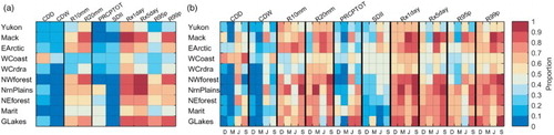
The BSS and CRPSS for each pair of grid points and the corresponding station were estimated. Figure 2 presents the corresponding values over each region. At the annual scale (yellow boxplots in Fig. 2), BSS and CRPSS were positive across all regions, meaning that the proposed LR and VGLM models outperformed forecasts based on climatology. However, performances differed among regions. Regions closer to large water bodies, as well as those with larger fractions of wet days (WCoast, NEforest, Marit, and GLakes), displayed better predictive skills (average BSS and CRPSS around 0.35) than central (NWforest and NrnPlains), mountainous (WCrdra), and northern regions (Yukon, Mack, and EArctic). The differences among regions could be attributed to the topography and the precipitation regime dominating those regions. Synoptic precipitation in regions on the east coast (NEforest, and Marit) and orographic precipitation in the WCoast region were better simulated by the reanalysis in terms of occurrence and intensity compared with the very dry northern and central regions dominated by less frequent and more likely convective precipitation. The Canadian Cordillera (WCrdra and part of the Mack and Yukon regions) also displayed a particular regime because precipitation is influenced by both the high elevation and the natural barrier to the westerlies which bring less moisture leeward. In these regions, some stations displayed lower BSS and CRPSS than elsewhere, which may be partly explained by the misrepresentation of the topography in CFSR due to its intrinsic spatial resolution, in addition to the fact that stations are usually located in valleys. Finally, Arctic regions displayed the lowest skill scores, though these were still positive. However, the network in Arctic regions has a lower density with unevenly distributed stations, making comparisons with other regions more difficult.

Fig. 2 Boxplots of (a) BSS and (b) CRPSS over each region and for each season. Numbers below each box plot indicate the number of stations within each region. Boxes delineate the interquartile range (IQR, [q₂₅ – q₇₅]), the horizontal line defines the median (q₅₀), while the limits of the lower and upper whiskers correspond, respectively, to q₂₅-1.5IQR and q₇₅ + 1.5IQR. Outliers are marked by black circles.

The precipitation regime impacted the forecast skill of the regression models at the seasonal scale for some regions (Fig. 2). During summer, most regions experience convective systems of short duration with relatively high intensity precipitation. Such systems are known to be partially resolved by numerical weather models both in terms of spatiotemporal resolution and underlying physical representation. As a result, CFSR was less efficient in representing those precipitation events. Therefore, BSS and CRPSS values were smaller in summer (JJA in Fig. 2) in the eastern (NEforest, Marit, and GLakes), the NrnPlains, and the WCoast regions. However, because autumn and winter (SON and DJF) are characterized by synoptic systems (i.e., systems of long duration and low intensity with relatively large spatial extent), they were more adequately represented by CFSR, as illustrated by the higher BSS and CRPSS values. It is worth noting that in the east (NEforest, GLakes, and Marit) and in the NrnPlains regions, BSS, and to a lesser extent CRPSS, displayed, on average, higher values during spring than winter and autumn. Northern regions displayed different seasonal patterns, with generally higher CRPSS and BSS during the summer than during winter. This may be partly related to the difficulty of measuring and simulating light precipitation during winter in Arctic regions, whereas summer wet synoptic system precipitation, which makes up a large fraction of the annual amount, was better simulated by CFSR. However, it seems reasonable to assume that reanalysis should not perform as well over the northern region where the volume of assimilated data is presumably smaller than for southern region.

c Performance of Post-Processed Precipitation Index Annual Series

Good performance was displayed by CFSR for some indices and regions in terms of reproducing the observed annual index distributions (ADKS test; see Section 4.b) as shown in Fig. 3a). Less than 50% of the sites in the central (NWforest and NrnPlains) and eastern (NEforest, Marit, and GLakes) regions had CFSR index distributions different from the observed distributions (95% c.l.) for R10mm, R20mm, Rx1day, Rx5day, R95p, and R99p. There was a greater contrast among results for these indices for northern (Yukon, Mack, and EArctic) and western (WCrdra, and WCoast) regions with generally better performance for Mack and EArctic regions. However, CFSR performed poorly for CDD, CDW, and SDII because only about 20% of the sites with CFSR distributions were not statistically different from observed distributions at the 95% c.l., the only exception being the WCoast region for the CDD indices. A more detailed analysis showed that the WCoast region could be subdivided into two regions with contrasting performances. The values of CDD at sites along the Pacific Ocean were very well estimated by CFSR, while CDD indices at the other sites located far from the coast were highly underestimated by the CFSR series. Finally, PRCPTOT was poorly represented in northern, western, and NWforest regions (only 20% of sites). Comparison of the CFSR and observed seasonal index distributions (Fig. 3b) indicates that CFSR performance depends strongly on the season with overall poorer performance in summer and autumn compared with winter and spring. Although observed annual distributions for some indices were quite well reproduced by CFSR (e.g., CDW), corresponding performance for some of the seasonal distributions was much less convincing. These results confirmed that daily CFSR precipitation series need to be post-processed for some regions before they can be used for the estimation of annual climate indices. The important issue is, therefore, to see whether post-processing of daily series improved the climate index distributions at sites where it was originally poor without significantly deteriorating the distributions at sites where it was originally good.

Fig. 3 (a) Proportion of sites within regions (rows) where observed and raw index (columns) distributions were not different at the 95% c.l. according to the ADKS tests; (b) as in (a) but at the seasonal scale. For clarity, D, M, J, and S refer to DJF, MAM, JJA, and SON, respectively.

Figure 4a.i summarizes the results of the comparisons between the post-processed and observed index distributions based on the ADKS test. The analysis was first conducted separately at sites where CFSR displayed both good and poor performance (Section 4.b), but regionally averaged percentages of post-processed index distributions were similar to the observed distributions. Thus, results for all sites were pooled in one figure, and results separating these two types of sites are presented in the supplemental material (Figs S1 and S2; supplemental material can be accessed at http://dx.doi.org/10.1080/07055900.2018.1434122). Figure 4a.i shows that on average, more than 90% of the post-processed annual index distributions obtained were similar to the observed distributions in many regions. This percentage was slightly lower for the R20mm, Rx1day, Rx5day, and R99p indices but was still between 60% and 70% for Rx5day and between 80% and 90% for the other indices. These percentages remained high for seasonal index distributions (Fig. 4a.ii), with, on average, more than 80%, and in many cases more than 90%, of the post-processed index distributions similar to the observed ones (95% c.l.), except during winter when a slight decrease in performance was observed compared with the other seasons. Seasonal and annual duration index (CDD and CDW) distributions were, on average, poorly reproduced over all regions as shown by the higher rejections of the ADKS null hypothesis, in all regions except Marit and GLakes. Winter and summer CDD index distributions were globally better reproduced, as 70% to 100% of the post-processed index distributions were not significantly different from observed distributions, while spring and autumn index distributions were better reproduced for CDW (60% to 80% of sites with not statistically different distributions). Eastern and central regions showed better results, on average, with high spatial variability in the performances within the same regions (not shown) unlike the other indices.

Fig. 4 Regional average of (a) the proportion of post-processed index distributions not different from the observed ones at the 95% c.l. according to the ADKS tests; (b) the relative bias between the post-processed and observed index series; (c) the NSTD; and (d) the NRMSE. The left panels (i) refer to the annual scale and right panels (ii) to the seasonal scale. For clarity, D, M, J, and S refer to DJF, MAM, JJA, and SON, respectively.

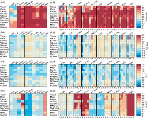
Results of the bias analysis (Fig. 4b.i) indicate that the index mean values were underestimated, on average, by less than 10% for intensity and frequency indices, except for PRCPTOT and SDII indices, for which slight overestimates were observed over the northern, central, and GLakes regions. The bias was higher (in absolute value) for the CDD and CDW indices with underestimates of around 30%, except in the eastern regions (≤10%). The seasonal frequency of days with more than 10 or 20 mm of precipitation, R10mm and R20mm, was relatively high in post-processed index series as illustrated in Fig. 4b.ii, especially in northern regions during winter and spring, which can be partly explained by the extremely small values of R10mm and R20mm (even zero in some years) over these regions. Biases between observed and CFSR indices were considerably reduced at sites where CFSR performance was poor and remained nearly unchanged (in absolute value) at sites where CFSR performance was already good, both for annual and seasonal index series (see Figs S3.a.i – S3.a.ii and S2.a.i – S2.a.ii) in the supplemental material). Interestingly, biases changed sign for CDW, going from highly overestimated values by CFSR (longer wet spells than observed) to underestimated values for post-processed indices, which may be partly explained by the lack of persistence of the post-processed daily precipitation series. Bias was lower during winter and summer for CDD and spring and autumn for CDW, except in the eastern regions, which displayed less marked seasonal differences and lower bias values.

The variability of post-processed annual index series was, in general, smaller than observed variability (NSTD values lower than one in Fig. 4c.i). Standard deviations for annual CDD and CDW index series were on average 20% to 30% smaller than for observed series over many regions with similar underestimates for the various seasons (Fig. 4c.ii). Slightly fewer underestimates of the interannual index variability were observed for the other indices with NSTD values around 0.8 for northern and western regions and close to 1.0 for central and eastern regions. The NSTD values were even slightly higher than 1.0 in the NrnPlains and GLakes for some indices for specific seasons (e.g., Rx1day in spring for the GLakes region). The R10mm and R20mm indices displayed highly under-dispersed series during winter, especially for northern and western regions. Here again, zero values in the observed index series may have an impact on these performances. Post-processing helped reduce the over-, or underestimates of the standard deviations in the annual and seasonal index series at sites with good and bad performances (Figs S3.b.i – S3.b.ii and S4.b.i – S4.b.ii) in the supplemental material).

Results for the NRMSE (Fig. 4d.i) indicate that PRCPTOT and SDII globally outperformed the other indices, followed by R95p and Rx5day. Overall, the extreme indices R99p, R95p, and Rx1day generated large NRSME values. The very small annual R20mm values and small seasonal R10mm and R20mm values observed in many regions, especially in winter, may partly explain the large reported NRMSE values for these indices (Fig. 4d.ii). Similar results were observed for R99p over all seasons. As indicated in Table 1, this index accounts for annual amounts greater than the observed 99th quantile. By construction R99p contained very high to very low (and even zero) values for both the observed and post-processed series, not necessarily occurring during the same year, leading to a very high NRMSE with good performance as regards averaged values of R99p during the study period (Figs 4a.ii and 4b.ii). Once again, the regionally averaged NRMSE between the observed and post-processed series were similar to those estimated with CFSR at sites where CFSR performed well, while they were considerably reduced at the other sites (Figs S3.c.i – S3.c.ii and S4.c.i – S4.c.ii in the supplemental material).

6 Conclusions

Reanalyses are constructed from numerical weather prediction models assimilating various observational datasets over a given historical period. However, reanalysis series should be post-processed in order to correct biases and possible spatial mismatch because of their resolution. In this study, stochastic post-processing (Wong et al., 2014) using CFSR daily precipitation as a covariate was applied locally to 1884 sites across Canada. This is the first step in the development of an approach in which precipitation series with local properties could be stochastically generated. Various applications require precipitation data at local scales, such as flood predictions (Vaittinada Ayar et al., 2016), impact studies (Maraun, 2016), agricultural modelling (Ambrosino et al., 2014), and water resource management. Enlarging the current post-processing approach at sites where reanalyses are available but without observations would also benefit the socio-economic and environmental development of regions with low station density. The post-processing was based on two regression approaches to model wet and dry day occurrences separately with an LR model and the daily precipitation intensities, represented by a gamma distribution, in a VGLM framework. Both models used the log-transformed CFSR daily precipitation as predictors and the observed daily occurrence (LR model) or intensity (VGLM) as predictand. Regression model parameters were also allowed to vary seasonally. The predictive power of the two regression models was first assessed separately through two skill scores, BSS and CRPSS for occurrences and intensities, respectively, using climatology as a reference dataset. The two models were then evaluated jointly by analyzing randomly generated series from the at-site daily precipitation distributions provided by the mixed distribution (occurrence and intensity). In this case, annual and seasonal climate series indices from the ETCCDI list (Peterson et al., 2001) allowed the study of further aspects of these post-processed precipitation sequences.

The probabilistic evaluation of the post-processing models showed systematically better forecast skill than the observed climatology for wet and dry occurrences and intensity, with regional and seasonal differences. Overall, BSS and CRPSS displayed similar regional patterns, with WCoast, NEForest, and Marit being the regions with the highest skill scores, especially during autumn and winter. Convection, characterizing summer precipitation in those regions, was more poorly represented by the models. The WCrdra and the central regions displayed lower skill scores, mainly explained by the topography and the small and infrequent occurrence of precipitation, respectively. Northern regions showed similar scores with better performance during summer (liquid precipitation). The other seasons are generally very dry, making the precipitation more difficult to measure (precipitation trace) and to be simulated by CFSR. Moreover, the paucity of assimilated weather data in the reanalysis may explain the poor performance of the models for those regions. Differences across regions and seasons also highlighted the importance of predictor choice (here CFSR precipitation and seasonal terms), because skill scores were consistently higher at sites where CFSR without post-processing already performed well (preliminary analysis not shown).

Annual and seasonal series of duration (CDD and CDW), frequency (R10mm and R20mm), and intensity (PRCPTOT, SDII, R95p, R99p, Rx1day, and Rx5day) indices were estimated from the randomly generated daily precipitation, referred to as post-processed series, and from recorded and CFSR daily series. The aim was to investigate whether post-processing was able to reproduce some of the observed precipitation attributes and to quantify the gain or loss of information by using post-processing instead of CFSR. This assessment was, all in all, the more interesting one because CFSR may already demonstrate good performance when dealing with upscaled series (e.g., annual amount series). The ADKS test conducted at the 95% c.l. compared at-site observed annual and seasonal index distributions with corresponding post-processed and CFSR index distributions. The three performance criteria B, NSTD, and NRMSE enabled further investigation of differences among these three datasets.

The main results follow:

• ADKS test showed CFSR index distributions were different (95% c. l.) from the observed ones for a large number of sites, especially for CDD, CDW, PRCPTOT, and SDII.

• For a given site, low percentages of post-processed CDD and CDW distributions were similar (according to the ADKS test) to observed distributions, especially in northern and western regions. These two indices were generally underestimated in the post-processed series. However, the absolute values of the bias were noticeably reduced when compared with CFSR. The post-processing showed some weaknesses for indices related to the duration of the wet and dry spells.

• The annual R10mm and R20mm distributions were well represented in the post-processed series, and bias was reduced when compared with CFSR. For some seasons, especially winter, R10mm and R20mm remained relatively low (even zero in some years) compared with observations and, therefore, performances (B, NSTD, and NRMSE) tended to be generally inferior.

• Intensity-related indices (PCRPTOT, SDII, Rx1day, Rx5day, R95p, and R99p) were the best-represented indices in the post-processed series for both annual and seasonal scales, especially for PCRPTOT, SDII, and to a lesser extent Rx1day and Rx5day. For the R95p and R99p distributions, relative bias and variability also displayed good performance when compared with the observed distributions. However, year-to-year errors were relatively high, especially for R99p because this index may contain both very low (zero values) and very high values, especially at seasonal time scales.

The post-processing provided very interesting corrections of the reanalysis, especially when one focuses on the distributions, as demonstrated by the ADKS results across upscaled precipitation indices. Moreover, the post-processed annual index series displayed considerably reduced bias and better estimates of interannual variability than those from CFSR, except for some indices in regions where the precipitation datasets, from either observations or reanalyses, were challenging to produce. Finally, although the NRMSE in post-processed series was reduced compared with CFSR, its values were generally elevated, suggesting that there is scope for further improvement with regard to the synchronicity between post-processed indices and the observed ones.

Preliminary analysis demonstrated that post-processing had very high skill when comparing statistics of at-site daily post-processed series, such as the mean, the variance, and a large range of quantiles (up to 95th), with those obtained from daily observed series. This highlighted that even if the gamma distribution is not recommended for use in representing the upper tail of the daily precipitation distribution, the VGLM framework, allowing a varying shape parameter, allowed for a tractable model and provided good estimates of moderately high quantiles. Future applications could involve the extended generalized Pareto proposed by Naveau, Huser, Ribereau, and Hannart (2016) to better represent quantiles of high order (>95th).

Future work should consider more persistence in the models, because the post-processed series partially reduced the CFSR autocorrelation. Several tests conducted with the same models, including CFSR precipitation on the previous day as a covariate, led to very similar results, suggesting another avenue of investigation (for example, integrating temporal structure in a latent field (Serinaldi & Kilsby (2014)). Moreover, a spatial structure of daily precipitation should be added to insure spatial consistency of the simulated random field, which was not investigated in this paper.

Table 1. Precipitation indices from the ETDCCI list computed at the annual and seasonal scales (Peterson et al., 2001).

Climate Index Identifier	Name	Description	Units
CDD	Consecutive dry days	Annual maximum number of consecutive dry days (<1 mm)	days
CWD	Consecutive wet days	Annual maximum number of consecutive wet days (≥1 mm)	days
R10 mm	Number of heavy precipitation days	Annual number of days with precipitation ≥10 mm	days
R20mm	Number of very heavy precipitation days	Annual number of days with precipitation ≥20 mm	days
PRCPTOT	Total wet day precipitation	Annual total precipitation	mm
SDII	Simple daily intensity index	Annual average precipitation on wet days (≥1 mm)	mm d^–1
Rx1day	Maximum 1-day precipitation	Annual maximum 1-day precipitation	mm
Rx5day	Maximum 5-day precipitation	Annual maximum 5-day precipitation	mm
R95p	Very wet days	Annual amount when daily precipitation is >95th percentile of the observed daily precipitation over the reference period	mm
R99p	Extremely wet days	Annual amount when daily precipitation is >99th percentile of the observed daily precipitation over the reference period	mm

Supplemental material

Supplemental data for this article can be accessed at http://dx.doi.org/10.1080/07055900.2018.143412210.

Acknowledgements

The authors would like to thank Eva Mekis from Environment and Climate Change Canada who provided the daily series from the Adjusted Precipitation for Canada (APC2) dataset, the Ministère du Développement Durable, de l’Environnement et de la Lutte contre les Changements Climatiques (MDDELCC) of Quebec (data available upon request; [email protected]) for the daily records, and Silvia Innocenti for advice on statistical tests. The authors also thank the two referees, Mohamed Ali Ben Alaya and Korbinian Breinl, for their constructive suggestions, which led to significant improvement of the manuscript.

Disclosure statement

No potential conflict of interest was reported by the authors.

Additional information

Funding

This research was partly funded by a Collaborative Research and Development Grant from the Natural Sciences and Engineering Research Council of Canada (NSERC).

Appendix: Statistical homogeneity of annual series

In this section, the protocol to check the statistical homogeneity is presented. In fact, some stations may have recording inconsistencies because of factors, such as changes in recording equipment, changes in the definition and measurement of precipitation trace (Mekis, 2005), missing values, choices of time windows to record daily precipitation (Hopkinson et al., 2011), and other site disturbances (Beaulieu et al., 2008). To further scrutinize the data, especially at stations that were not part of the APC2 dataset, the statistical homogeneity of annual precipitation series was also assessed using the method proposed by Wijngaard, Klein Tank, and Konnen (2003), which relies on the application of four statistical tests. The sites with homogeneous series classified as “useful” according to the terminology of Wijngaard et al. (2003), were selected (in these cases three or more of the tests do not reject the null hypothesis that the temporal series are independently and identically distributed at the 99% level). Though, some useful gauging stations were discarded because they displayed an increasing annual number of wet days over time, whereas the recording resolution was also increasing, leading to spurious trends. Twenty-two stations in southern Saskatchewan were not considered because of numerous missing years over the study period, despite the quality control applied.

References

- Akaike, H. (1974). A new look at the statistical model identification. IEEE Transactions on Automatic Control, 19, 716–723. doi: 10.1109/TAC.1974.1100705
- Allard, M., & Lemay, M. (2012). Nunavik and Nunatsiavut: From science to policy. An Integrated Regional Impact Study (IRIS) of climate change and modernization. Québec: ArcticNet Inc. Retrieved from http://arcticnet.ulaval.ca/pdf/media/iris_Teport_complete.pdf
- Ambrosino, C., Chandler, R. E., & Todd, M. C. (2014). Rainfall-derived growing season characteristics for agricultural impact assessments in South Africa. Theoretical and Applied Climatology, 115(3-4), 411–426. doi: 10.1007/s00704-013-0896-y
- Asong, Z. E., Khaliq, M. N., & Wheater, H. S. (2016a). Multisite multivariate modeling of daily precipitation and temperature in the Canadian Prairie Provinces using generalized linear models. Climate Dynamics, 47, 2901–2921. doi: 10.1007/s00382-016-3004-z
- Asong, Z. E., Khaliq, M. N., & Wheater, H. S. (2016b). Projected changes in precipitation and temperature over the Canadian Prairie Provinces using the generalized linear model statistical downscaling approach. Journal of Hydrology, 539, 429–446. doi: 10.1016/j.jhydrol.2016.05.044
- Beaulieu, C., Seidou, O., Ouarda, T. B. M. J., Zhang, X., Boulet, G., & Yagouti, A. (2008). Intercomparison of homogenization techniques for precipitation data. Water Resources Research, 44, W02425. doi: 10.1029/2006WR005615
- Ben Alaya, M. A., Ouarda, T. B. M. J., & Chebana, F. (2018). Non-Gaussian spatiotemporal simulation of multisite daily precipitation: Downscaling framework. Climate Dynamics, 50, doi: 10.1007/S00382-017-3578-0
- Bengtsson, L., & Shukla, J. (1988). Integration of space and in situ observations to study global climate change. Bulletin of the American Meteorological Society, 69, 1130–1143. doi: 10.1175/1520-0477(1988)069<1130:IOSAIS>2.0.CO;2
- Bentzien, S., & Friederichs, P. (2014). Decomposition and graphical portrayal of the quantile score. Quarterly Journal of the Royal Meteorological Society, 140(683), 1924–1934. doi: 10.1002/qj.2284
- Bosilovich, M. G., Chen, J., Robertson, F. R., & Adler, R. F. (2008). Evaluation of global precipitation in reanalyses. Journal of Applied Meteorology and Climatology, 47(9), 2279–2299. doi: 10.1175/2008JAMC1921.1
- Bromwich, D. H., Nicolas, J. P., & Monaghan, A. J. (2011). An assessment of precipitation changes over Antarctica and the Southern Ocean since 1989 in contemporary global reanalyses. Journal of Climate, 24(16), 4189–4209. doi: 10.1175/2011JCLI4074.1
- Buishand, T. A., Shabalova, M. V., & Brandsma, T. (2004). On the choice of the temporal aggregation level for statistical downscaling of precipitation. Journal of Climate, 17(9), 1816–1827. doi: 10.1175/1520-0442(2004)017<1816:OTCOTT>2.0.CO;2
- Canadian Space Agency (CSA). (2012). Technical guide development, interpretation, and use of rainfall Intensity-Duration-Frequency (IDF) information: Guideline for Canadian water resources practioners ( Technical Guide Plus 4013-12). Mississauga, ON: Author.
- Chandler, Wheater, H. S. (2002). Analysis of rainfall variability using generalized linear models: A case study from the west of Ireland. Water Resources Research, 38(10), 10-1–10-11. doi: 10.1029/2001WR000906
- Chandler, R. E. (2002). GLIMCLIM: Generalized Linear Modelling for Daily Climate time series (software and user guide) ( Tech. Rep. No. MSU-CSE-00-2). Department of Statistical Science, University College London.
- Coe, R., & Stern, R. (1982). Fitting models to daily rainfall data. Journal of Applied Meteorology, 21(7), 1024–1031. doi: 10.1175/1520-0450(1982)021<1024:FMTDRD>2.0.CO;2
- Conover, W. (1999). Practical nonparametric statistics (3rd ed.). New York, NY: John Wiley & Sons.
- Contractor, S., Alexander, L. V., Donat, M. G., & Herold, N. (2015). How well do gridded datasets of observed daily precipitation compare over Australia? Advances in Meteorology, 2015, 325718. doi: 10.1155/2015/325718
- Dai, A. (2006). Precipitation characteristics in eighteen coupled climate models. Journal of Climate, 19(18), 4605–4630. doi: 10.1175/JCLI3884.1
- Devine, K. A., & Mekis, E. (2008). Field accuracy of Canadian rain measurements. Atmosphere-Ocean, 46(2), 213–227. doi: 10.3137/ao.460202
- Donat, M. G., Sillmann, J., Wild, S., Alexander, L. V., Lippmann, T., & Zwier, F. W. (2014). Consistency of temperature and precipitation extremes across various global gridded in situ and reanalysis datasets. Journal of Climate, 27(13), 5019–5035. doi: 10.1175/JCLI-D-13-00405.1
- Eden, J. M., Widmann, M., Maraun, D., & Vrac, M. (2014). Comparison of GCM- and RCM-simulated precipitation following stochastic postprocessing. Journal of Geophysical Research: Atmospheres, 119(19), 11,040–11,053.
- Environment and Climate Change Canada. (2013). Adjusted Precipitation and Homogenized Canadian Climate Data (AHCCD). Retrieved from http://ec.gc.ca/dccha-ahccd/default.asp?lang=En&n=9AA530BE-1
- Eum, H.-I., Cannon, A. J., & Murdock, T. Q. (2017). Intercomparison of multiple statistical downscaling methods: Multi-criteria model selection for South Korea. Stochastic Environmental Research and Risk Assessment, 31(3), 683–703. doi: 10.1007/s00477-016-1312-9
- Eum, H.-I., Dibike, Y., Prowse, T., & Bonsal, B. (2014). Inter-comparison of high-resolution gridded climate data sets and their implication on hydrological model simulation over the Athabasca Watershed, Canada. Hydrological Processes, 28(14), 4250–4271. doi: 10.1002/hyp.10236
- Fowler, H., Blenkinsop, S., & Tebaldi, C. (2007). Linking climate change modelling to impacts studies: Recent advances in downscaling techniques for hydrological modelling. International Journal of Climatology, 27(12), 1547–1578. doi: 10.1002/joc.1556
- Friederichs, P., & Thorarinsdottir, T. L. (2012). Forecast verification for extreme value distributions with an application to probabilistic peak wind prediction. Environmetrics, 23(7), 579–594. doi: 10.1002/env.2176
- Gervais, M., Tremblay, L. B., Gyakum, J. R., & Atallah, E. (2014). Representing extremes in a daily gridded precipitation analysis over the United States: Impacts of station density, resolution, and gridding methods. Journal of Climate, 27(14), 5201–5218. doi: 10.1175/JCLI-D-13-00319.1
- Hersbach, H. (2000). Decomposition of the continuous ranked probability score for ensemble prediction systems. Weather and Forecasting, 15(5), 559–570. doi: 10.1175/1520-0434(2000)015<0559:DOTCRP>2.0.CO;2
- Higgins, R. W., Kousky, V. E., Silva, V. B. S., Becker, E., & Xie, P. (2010). Intercomparison of daily precipitation statistics over the United States in observations and in NCEP reanalysis products. Journal of Climate, 23(17), 4637–4650. doi: 10.1175/2010JCLI3638.1
- Hofstra, N., New, M., & McSweeney, C. (2010). The influence of interpolation and station network density on the distributions and trends of climate variables in gridded daily data. Climate Dynamics, 35(5), 841–858. doi: 10.1007/s00382-009-0698-1
- Hopkinson, R. F., Mckenney, D. W., Milewska, E. J., Hutchinson, M. F., Papadopol, P., & Vincent, L. A. (2011). Impact of aligning climatological day on gridding daily maximum-minimum temperature and precipitation over Canada. Journal of Applied Meteorology and Climatology, 50(8), 1654–1665. doi: 10.1175/2011JAMC2684.1
- Kalnay, E., Kanamitsu, M., Kistler, R., Collins, W., Deaven, D., Gandin, L., … Joseph, D. (1996). The NCEP/NCAR 40-year reanalysis project. Bulletin of the American Meteorological Society, 77(3), 437–471. doi: 10.1175/1520-0477(1996)077<0437:TNYRP>2.0.CO;2
- Katz, R. W. (1977). Precipitation as a chain-dependent process. Journal of Applied Meteorology, 16(7), 671–676. doi: 10.1175/1520-0450(1977)016<0671:PAACDP>2.0.CO;2
- Lavers, D., Prudhomme, C., & Hannah, D. M. (2013). European precipitation connections with large-scale mean sea-level pressure (mslp) fields. Hydrological Sciences Journal, 58(2), 310–327. doi: 10.1080/02626667.2012.754545
- Maraun, D. (2013). Bias correction, quantile mapping, and downscaling: Revisiting the inflation issue. Journal of Climate, 26(6), 2137–2143. doi: 10.1175/JCLI-D-12-00821.1
- Maraun, D. (2016). Bias correcting climate change simulations - a critical review. Current Climate Change Reports, 2(4), 211–220. doi: 10.1007/s40641-016-0050-x
- Maraun, D., Wetterhall, F., Ireson, A. M., Chandler, R. E., Kendon, E. J., Widmann, M., … Thiele-Eich, I. (2010). Precipitation downscaling under climate change: Recent developments to bridge the gap between dynamical models and the end user. Reviews of Geophysics, 48(3), 1–34. doi: 10.1029/2009RG000314
- Maraun, D., Widmann, M., Gutierrez, J. M., Kotlarski, S., Chandler, R. E., Hertig, E., … Wilcke, R. A. (2015). VALUE: A framework to validate downscaling approaches for climate change studies. Earth’s Future, 3(1), 1–14. doi: 10.1002/2014EF000259
- McCullag, P., & Nelder, J. A. (1989). Generalized linear models (2nd ed.). New York, NY: Chapman and Hall.
- Mekis, E. (2005). Adjustments for trace measurements in Canada. Proceedings of the 15th conference on applied climatology, June 2005, Savannah, Georgia, USA, 6 pp.
- Mekis, E., & Vincent, L. A. (2011). An overview of the second generation adjusted daily precipitation dataset for trend analysis in Canada. Atmosphere-Ocean, 49(2), 163–177. doi: 10.1080/07055900.2011.583910
- Mesinger, F., DiMego, G., Kalnay, E., Mitchell, K., Shafran, P. C., Ebisuzaki, W., … Shi, W. (2006). North American Regional Reanalysis. Bulletin of the American Meteorological Society, 87(3), 343–360. doi: 10.1175/BAMS-87-3-343
- Metcalfe, J., Routledge, B., & Devine, K. (1997). Rainfall measurement in Canada: Changing observational methods and archive adjustment procedures. Journal of Climate, 10(1), 92–101. doi: 10.1175/1520-0442(1997)010<0092:RMICCO>2.0.CO;2
- Naveau, P., Huser, R., Ribereau, P., & Hannart, A. (2016). Modeling jointly low, moderate, and heavy rainfall intensities without a threshold selection. Water Resources Research, 52(4), 2753–2769. doi: 10.1002/2015WR018552
- Neykov, N. M., Neytchev, P. N., & Zucchini, W. (2014). Stochastic daily precipitation model with a heavy-tailed component. Natural Hazards and Earth System Science, 14(9), 2321–2335. doi: 10.5194/nhess-14-2321-2014
- Peterson, T. C., Folland, C., Gruza, G., Hogg, W., Mokssit, A., & Plummer, N. (2001). Report on the activities of the working group on climate change detection and related rapporteurs 1998-2001 (Technical Report WMO-TD11071). Geneva, WMO, Retrieved from http://etccdi.pacificclimate.org/docs/wgccd.2001.pdf
- Piani, C., Haerter, J. O., & Coppola, E. (2010). Statistical bias correction for daily precipitation in regional climate models over Europe. Theoretical and Applied Climatology, 99(1-2), 187–192. doi: 10.1007/s00704-009-0134-9
- Plummer, D. A., Caya, D., Frigon, A., Cote, H., Giguere, M., Paquin, D., … de Elia, R. (2006). Climate and climate change over North America as simulated by the Canadian RCM. Journal of Climate, 19(13), 3112–3132. doi: 10.1175/JCLI3769.1
- Rusticucci, M., Zazulie, N., & Raga, G. B. (2014). Regional winter climate of the southern central Andes: Assessing the performance of ERA-Interim for climate studies. Journal of Geophysical Research: Atmospheres, 119(14), 8568–8582.
- Saha, S., Moorthi, S., Pan, H.-L., Wu, X., Wang, J., Nadiga, S., … Goldberg, M. (2010). The NCEP climate forecast system reanalysis. Bulletin of the American Meteorological Society, 91(8), 1015–1058. doi: 10.1175/2010BAMS3001.1
- Schmidli, J., Frei, C., & Vidale, P. L. (2006). Downscaling from GCM precipitation: A benchmark for dynamical and statistical downscaling methods. International Journal of Climatology, 26(5), 679–689. doi: 10.1002/joc.1287
- Serinaldi, F., & Kilsby, C. G. (2014). Simulating daily rainfall fields over large areas for collective risk estimation. Journal of Hydrology, 512, 285–302. doi: 10.1016/j.jhydrol.2014.02.043
- Stern, R. D., & Coe, R. (1984). A model fitting analysis of daily rainfall data. Journal of the Royal Statistical Society. Series A (General), 147(1), 1–34. doi: 10.2307/2981736
- Sun, Y., Solomon, S., Dai, A., & Portmann, R. W. (2006). How often does it rain? Journal of Climate, 19(6), 916–934. doi: 10.1175/JCLI3672.1
- Tustison, B., Harris, D., & Foufoula-Georgiou, E. (2001). Scale issues in verification of precipitation forecasts. Journal of Geophysical Research: Atmospheres, 106(D11), 11775–11784. doi: 10.1029/2001JD900066
- Vaittinada Ayar, P., Vrac, M., Bastin, S., Carreau, J., Deque, M., & Gallardo, C. (2016). Intercomparison of statistical and dynamical downscaling models under the EURO- and MED-CORDEX initiative framework: Present climate evaluations. Climate Dynamics, 46(3), 1301–1329. doi: 10.1007/s00382-015-2647-5
- Vrac, M., & Naveau, P. (2007). Stochastic downscaling of precipitation: From dry events to heavy rainfalls. Water Resources Research, 43, W07402. doi:10.01029/2006WR005388 doi: 10.1029/2006WR005308
- Way, R. G., Oliva, F., & Viau, A. E. (2017). Underestimated warming of northern Canada in the Berkeley earth temperature product. International Journal of Climatology, 37(4), 1746–1757. doi: 10.1002/joc.4808
- Wijngaard, J. B., Klein Tank, A. M. G., & Konnen, G. P. (2003). Homogeneity of 20th century European daily temperature and precipitation series. International Journal of Climatology, 23(6), 679–692. doi: 10.1002/joc.906
- Wilks, D. (2011). Statistical methods in the atmospheric sciences (3rd ed.). New York: Academic Press.
- Wilks, D., & Wilby, R. L. (1999). The weather generation game: A review of stochastic weather models. Progress in Physical Geography, 23(3), 329–357. doi: 10.1177/030913339902300302
- Wong, G., Maraun, D., Vrac, M., Widmann, M., Eden, J. M., & Kent, T. (2014). Stochastic model output statistics for bias correcting and downscaling precipitation including extremes. Journal of Climate, 27(18), 6940–6959. doi: 10.1175/JCLI-D-13-00604.1
- Yee, T. W. (2016). VGAM: Vector generalized linear and additive models [Computer software manual]. (R package version 1.0-3). Retrieved from http://CRAN.R-project.org/package=VGAM
- Yee, T. W., & Wild, C. J. (1996). Vector Generalized Additive Models. Journal of the Royal Statistical Society. Series B (Methodological), 58(3), 481–493.
- Zhang, Q., Kornich, H., & Holmgren, K. (2013). How well do reanalyses represent the Southern African precipitation? Climate Dynamics, 40(3-4), 951–962. doi: 10.1007/s00382-012-1423-z