Evaluation of the Influence of Aquatic Plants and Lake Bottom on the Remote-Sensing Reflectance of Optically Shallow Waters

Abstract

Aquatic plants and lake bottoms in optically shallow waters (OSWs) wield great influence on reflectance spectra, resulting in the inapplicability of most existing bio-optical models for water colour remote sensing in lakes. Based on radiative transfer theory and measured spectra from a campaign for Lake Taihu in October 2008, absorption and backscattering coefficients were used to simulate the remote-sensing reflectance, which are considered to be reliable if matched to their measured counterparts. Several cases of measured spectra at different depths, Secchi disk depth transparency, and aquatic plant height and coverage were analyzed thoroughly for spectral properties. The contribution of aquatic plants was evaluated and compared with the measured and simulated remote-sensing reflectance values. This is helpful for removing the influence of aquatic plants and lake bottoms from the spectra and for constructing an improved chlorophyll a retrieval model for OSWs, such as that for Lake Taihu, China.

Résumé

[Traduit par la rédaction] Les plantes aquatiques et les fonds de lacs en eaux optiquement peu profondes influent grandement sur les spectres de réflectance et rendent inapplicables la plupart des modèles bio-optiques existants en ce qui concerne la télédétection de la couleur de l’eau dans les lacs. Sur la base de la théorie du transfert radiatif et des spectres mesurés lors d’une campagne au lac Taihu en octobre 2008, nous avons utilisé les coefficients d’absorption et de rétrodiffusion pour simuler la réflectance détectée à distance. Ces deux facteurs sont considérés comme étant fiables s’ils correspondent à leur équivalent mesuré. Nous avons analysé minutieusement plusieurs cas de spectres mesurés à diverses profondeurs, profondeur de transparence mesurée au disque de Secchi et hauteur des plantes aquatiques, et de couverture afin d’en déterminer les propriétés spectrales. Nous avons évalué la contribution des plantes aquatiques et l’avons comparée aux valeurs de réflectance détectée à distance, tant mesurées que simulées. Cette méthode permet d’éliminer l’influence des plantes aquatiques et des fonds de lacs sur les spectres et de construire un modèle amélioré d’extraction de chlorophylle a pour les eaux optiquement peu profondes, comme celles du lac Taihu, en Chine.

Keywords:

• aquatic plants
• optically shallow waters
• remote-sensing reflectance
• turbid waters

1 Introduction

The ultimate goal of water colour remote sensing is to estimate the contents and concentrations of water constituents (Duan, Ma, & Hu, 2012; Koponen et al., 2001; Woźniak et al., 1999, 2005). When sunlight penetrates the water surface and moves down through the water column, portions of the electromagnetic energy are absorbed and scattered at rates determined by, in addition to pure water, the concentrations of coloured dissolved and particulate matter that make up the water mixture (Dekker, Vos, & Peters, 2001; Duan et al., 2015; Pulliainen et al., 2001; Zhang et al., 2009a, 2009b). In shallow waters, where the depth is much less than the potential for light to penetrate, a large fraction of the subsurface light reaches the bottom, where portions of the light energy are absorbed, reflected into the overlying water column, or re-emitted as fluorescence (Henderson et al., 2009; Liu et al., 2015). The subsurface light field in shallow water is a function not only of the properties of the water mixture but also of the depth and properties of the bottom. Depending on depth and benthic optical properties, light intensity might decrease more rapidly than expected, remain constant throughout the water column, or even increase with depth (Hedley, Roelfsema, & Phinn, 2009; Li, Liu, & Gu, 2010; Maritorena, Morel, & Gentili, 1994). Therefore, a large difference exists between optically deep waters (ODWs) and optically shallow waters (OSWs). The reflectance in ODWs is dominated by the inherent optical properties (IOPs) of the water constituents (Ceyhun & Yalcin, 2010; Gordon, Brown, & Jacobs, 1975; Mobley, 1994; Zhang et al., 2009a), while in OSWs, in addition to the effects of IOPs, the interaction between light propagation and the underlying surface influences the water colour signal to a large extent. Researchers cannot neglect this (Lee & Carder, 2005; Li et al., 2010; Shi et al., 2015; Zhang et al., 2009a). In the present study, we examine two areas representative of these types of waters: an aquatic plant area (i.e., the eastern part of Lake Taihu, or OSWs) and a non-aquatic plant area (i.e., ODWs). Lodhi and Rundquist (2001) mentioned that the bottom effect on the upwelling spectral signal may be considered insignificant where the depth of the water is more than three times the observed Secchi disk depth (SDD); these waters are defined as ODWs. In all other cases, the waters are OSWs, meaning the spectra would most likely be influenced by both the bottom and aquatic plants (Hedley, Roelfsema, Phinn, & Mumby, 2012; Jiang, Jin, Yao, Li, & Wu, 2008; Luo et al., 2016).

Because most retrieval algorithms that have been developed are suitable for ODWs, little consideration is necessary for the contribution of aquatic plants to water-leaving signals. When using remotely sensed data, water-quality concentrations such as chlorophyll a (chl a) values are overestimated in aquatic plant areas (Hedley, 2008; Jiang et al., 2008; Ma & Dai, 2005; Ritchie & Cooper, 1991). To enhance the retrieval estimation accuracy of water-quality parameters, determining characteristics, as well as estimating the contributions of aquatic plants and the bottom, become crucial issues in clear shallow waters.

In this regard, most previous research has been conducted using simulation methods. Maritorena et al. (1994) gave an approximate solution of irradiance reflectance just below the surface based on the radiative transfer equation, taking into consideration the contributions expected from both the water column and the bottom. Then Lee et al. (1998) developed a semi-analytical model to simulate the remote-sensing reflectance above (R_rs) and below (r_rs) the surface for various combinations of optical properties, including bottom albedos, bottom depths, and solar zenith angles; thus, the contribution to the remotely sensed signal from the water column could be separated from that of the bottom. They found that the spectra determined by the semi-analytical model showed good agreement with the exact spectra computed using the radiative transfer program Hydrolight. Soon after, Lee, Carder, Mobley, Steward, and Patch (1999) modified the model with optimized parameters, using the Hydrolight simulation based on single or quasi-single-scattering theory and deriving bottom depths and water properties through optimization. Albert and Mobley (2003) developed an analytical model to investigate the surface remote-sensing signals based on simulations with Hydrolight using the optical properties of Lake Constance, Germany. In comparison, the model is more comprehensive, with solar zenith angle, viewing angle, and surface wind speed taken into account.

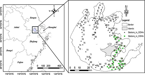
Lake Taihu is the third-largest freshwater lake in China (Wang, 1985), and borders the provinces of Shanghai, Jiangsu, and Zhejiang (Fig. 1). It is also an important source of drinking water for several developed cities nearby (e.g., Shanghai, Wuxi, and Suzhou). Lake Taihu covers an area of 2427.8 km². The average depth is about 1.9 m, with a maximum of 2.6 m (Qin, Hu, & Chen, 2004; Zhang, van Dijk, Liu, Zhu, & Qin, 2009b), which varies slightly in different seasons. The lake, which connects other springs, lakes, and rivers, forming the heart of a very important water network in South China, eventually flows into the Yangtze River. In this study, we investigate the contributions of aquatic plants and lake bottom to the remote-sensing reflectance, using in situ data measured at about 30 sites in the OSWs of Lake Taihu in October 2008. In particular, we analyze the spectra at different sites, categorize them into several water types, and compare the measured R_rs with the simulated R_rs spectra. The analysis results are then compared with those of Ma, Duan, Zhang, and Pan (2008) and are also compared with measurements in October 2010 (Duan et al., 2012).

Fig. 1 Location of Lake Taihu, the study area. The ODW and OSW sites are shown on the map.

2 Data acquisition and methodology

a Field Measurements

Field measurements were carried out in the study area at Lake Taihu as shown in Fig. 1. In the eastern part of the lake (i.e., in the OSWs) the water depth is shallow (varying from 1.4 m to 2.5 m) and the water is very clear (SDD from 0.5 m⁻¹ to 1.75 m⁻¹); hence, the aquatic plants and the lake bottom greatly influence the reflectance spectra measured at the surface, resulting in the unavailability of most in situ remote-sensing reflectance measurements for the OSWs. This poses a great challenge; more attention is needed to quantify and assess the contributions of aquatic plants and the lake bottom to the reflectance spectra to make satellite remote sensing more effective for use as an assessment tool.

Water samples, in situ optical data, and spectral measurements at 100 selected sites were collected around Lake Taihu between 5 and 17 October 2008. Optical data including upwelling and downwelling irradiance, upwelling radiance, and remote-sensing reflectance were measured, as well as backscattering coefficients, SDD, wind direction, and wind speed. To measure the concentrations of chl a, total suspended sediment, and dissolved organic carbon (DOC), water samples were collected in polyethylene bottles and refrigerated for laboratory analysis. Laboratory measurements were also obtained for the absorption coefficients of the total particles, phytoplankton, detritus, and coloured dissolved organic matter (CDOM). Eventually, a dataset of optical water-quality parameters was obtained, as well as spectral data using both surface and water column sampling from optical instruments and carefully following their operation instructions. Based on the definition of OSWs (Lodhi & Rundquist, 2001), 30 sites in the eastern part of Lake Taihu were chosen, as shown in Fig. 1.

1 data acquisition from field observation

The dual spectrometer, ASD FieldSpec® Pro Dual VNIR (FieldSpec 931 from ASD Ltd., America) was used to measure water-leaving radiance (L_W), one of the apparent optical properties, and sky radiance (L_sky) emitted from the water surface and sky by following the ocean optics protocols of the National Aeronautics and Space Administration (NASA; Mueller et al., 2003). The viewing angles from the water surface for the zenith and azimuth were 40° and 135°, respectively. The sequence involved measuring a 25 cm by 25 cm plaque with 25% reflectivity radiance and water and sky radiances (each preceded by a dark offset reading); this was replicated five times. The measurements were taken at a location that minimized shade, reflections from superstructure, ships’ wakes, and other related foam patches and whitecaps. Moreover, the viewed location was pointed away from the sun to reduce the specular reflection of sunlight. With the upward radiance (L_u), sky radiance (L_sky), and grey plaque radiance (L_plaq), the remote-sensing reflectance R_rs can be calculated using software produced by colleagues at Nanjing Institute of Geography and Limnology. For more information, see Ma et al. (2006).

The total backscattering coefficients (b_b), including the contribution from pure water, were measured with a HydroScat-6 Spectral Backscattering Sensor (HS6) at six wavelengths: 420, 442, 470, 510, 590, and 700 nm. Before the campaign started, the unit was calibrated following procedures from the Backscattering Sensor Calibration manual (HOBI-labs Inc. 2008).

2 Data from Laboratory Analysis

Concentrations of chl a were measured with the spectrophotometric determination method following NASA ocean optics protocols (Mueller et al., 2003). Total suspended sediment (TSS) concentrations were determined gravimetrically from samples collected on the pre-combusted and pre-weighted GF/F filters and dried at 95°C overnight. The suspended substance filters were burned at 550°C for three hours to differentiate TSS into inorganic suspended sediment and organic suspended sediment (OSS). Concentrations of DOC were measured with a type of 1020 total organic carbon equipment (OI Corp., College Station, TX) after water samples were filtered through Whatman GF/F glass fibre filters.

Absorption coefficients of the total particulates (a_p) were measured by concentrating the particulate onto a filter, a method proposed by Yentsch (1962). Then the total particulate absorption was separated into pigment (a_ph) and detritus absorption (a_d) by extracting the filter in methanol. Mitchell (1990) named this method the quantitative filter technique (QFT). The absorption (a_g) of CDOM was measured spectrophotometrically in a 10 cm cuvette using 0.70 mm Whatman GF/F-filtered lake water and the same UV-2401 spectrophotometer, with distilled water as a reference. Scans were taken at intervals of 1 nm from 280 to 700 nm. The absorption coefficients of pure water, in the range of 380–700 nm, were adopted from Pope and Fry (1997).

b Simulated Remote-Sensing Reflectance

1 simulation method and data input

Based on radiative transfer theory, the following relationship can be obtained:(1) where λ is the wavelength, the ratio f/Q is dependent on the sun’s position (Morel & Gentili, 1993), n is the water refraction coefficient (usually taken as 1.34), and t is the permeability of the water–atmosphere interface. From Clark (1981), t/n² is given the value 0.54, and a(λ) and b_b(λ) are the total absorption coefficient and total backscattering coefficient of the water column, respectively.

From previous knowledge we have acquired, a(λ) and b_b(λ) can be divided into the contributions from pure water (w), total particulate matter (p), and CDOM. Equation (1) thus becomes(2) Obviously, f/Q, a(λ), and b_b(λ) should first be determined in order to simulate R_rs(λ).

i Optical factors f and Q

Usually the factors Q and f are determined empirically or via simulation (Gons, 1999; Zhang et al., 2009a). It should be noted that the values might be slightly different in different sampling areas and different years. Depending on the Monte Carlo studies (Kirk, 1994), f could be expressed as a linear function of μ₀:(3) where μ₀ is the mean cosine of the angle that the photons make with the vertical just beneath the water surface. The value of μ₀ is calculated according to the sampling time, latitude, and solar altitude angle; Q is inversely related to μ₀, ranging from 0.3 to 6.5, but is generally expected to be 3–4 (Morel & Gentili, 1993). Here we use the empirical equation Q = 2.38/μ₀ to calculate Q (Gons, 1999). Depending on the theories above, the mean values of f/Q in winter, spring, summer, and autumn in Lake Taihu are 0.158, 0.153, 0.152, and 0.157, respectively (Zhang et al., 2009a). However, based on in situ measurements in our campaign of October 2008, f/Q has a calculated mean of 0.154. Henceforth, we use this value in the simulation of R_rs(λ).

ii Spectra of total absorption coefficient a(λ)

The total absorption can be obtained by summing all the absorption coefficients of different water constituents. For pure fresh water, the absorption coefficient of pure water a_w(λ) is obtained from Smith and Baker (1981). The wavelength interval for a_w(λ) is 10 nm while our in situ absorption spectra have a 1 nm spectral resolution. The a_w(λ) spectra of Smith and Baker (1981) are then interpolated into 1 nm using linear interpolation. Based on the spectral curve, a_w(λ) increases continually from 400 to 760 nm. Differing from a_w(λ), both a_p(λ) and a_CDOM(λ) have a decreasing trend with wavelength in the visible and near-infrared regions; they are very close to zero at about 750 nm. The total absorption spectra a(λ) at all available sites are calculated by summing the above three absorptions. In Fig. 2 (left), a(λ) shows a similar trend to a_p(λ) in the range 400–700 nm because the a_p(λ) signals in this region are strong and dominant. However, at wavelengths longer than 700 nm, a_w(λ) begins contributing most to a(λ), and the a(λ) spectra at all available sites gradually converge into a single line with a magnitude and trend similar to the a_w(λ) spectra in the lake.

Fig. 2 Total absorption spectra a(λ) (left) and total backscattering coefficients b_b(λ) (right) at all available sites in Lake Taihu.

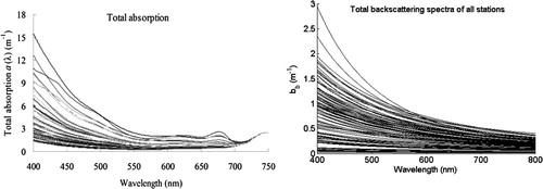
iii Spectra of the total backscatter coefficient b_b(λ)

The total backscatter coefficients (b_b), including the contribution from pure water (b_w), were measured with a HydroScat-6 Spectral Backscattering Sensor (HS-6) at six wavelengths, centred at 420, 442, 470, 510, 590, and 700 nm. Values for b_w(λ) are taken from the data of Buiteveld, Hakvoort, and Donze (1994); its spectral curve has a decreasing trend from 400 to 800 nm. By subtracting b_w(λ) from b_b(λ) at the six wavelengths, b_bp(λ) at 420, 442, 470, 510, 590, and 700 nm can be obtained. Because the b_bp(λ) spectra have a decreasing trend with wavelength, b_bp(λ) over the visible wavelength range can be simulated, depending on measured values, using a power function. Taking 510 nm as the reference wavelength corresponding to the mounted band in the HS-6, it can be expressed as(4) where Y is an exponent defining the wavelength dependence of particulate scattering; it can be directly related to the particle grain-size distribution and can also be calculated using the measured b_bp(510). Together with the backscattering coefficients of pure water, the total backscattering spectra are then obtained in the entire wavelength range at each site (Fig. 2 (right)). Because of the small contribution from pure water, the total backscattering spectra from 400 to 800 nm are similar to b_bp(λ), with only a small difference in magnitude.

2 simulated R_rs(λ) and reliability analysis

With the data determined above substituted into Eq. (2), the simulated R_rs(λ) can be calculated for all the available sites. The spectral shape and property of the simulated R_rs(λ) in both ODWs and OSWs are all rational compared with the in situ measured R_rs(λ). However, the simulated spectra should be compared, in more detail, with the measured ones in several aspects to determine whether they are reliable for further utilization. These include spectral shape and variation, peak position, and magnitude. It should be noted, however, that the measured R_rs(λ) at sites with high chl a or cyanophycin granules or aquatic plants proved invalid in estimating chl a contents. Thus, in validating the reliability of the simulated R_rs(λ), we discarded the data in these areas, only choosing those spectra in the ODWs for which the chl a concentrations were no more than 110 mg m^-3. To simplify the comparison, nine sites were chosen with different magnitudes of chl a concentration. Table 1 gives the sites and their corresponding chl a concentrations, which vary from 8.97 to 108.9 mg m^-3.

Table 1. Selected sites and their corresponding chl a concentrations.

Site No.	3	4	63	70	80	85	87	97	100
chl a (mg m^−3)	108.90	27.21	8.97	31.24	80.05	43.56	15.91	47.82	97.39

i Spectral variation and shape

First, the standard deviation (SD) distributions of the measured and simulated spectra at all sites are compared. It is well known that the SD of a dataset is the square root of its variance and is widely used to measure the variability or dispersion of the dataset. It shows how much variation there is from the average or mean value. A low SD indicates that the data points tend to be very close to the average, whereas a high SD means the data are spread over a large range of values. The SD spectra of both measured and simulated R_rs(λ) for all sites are plotted in Fig. 3a. It can be clearly seen that in the 440–800 nm range, the SD values of the simulated spectra are lower than those of the measured spectra, which indicates that the simulated R_rs(λ) are less dispersed than the measured R_rs(λ). The most probable reason is that, with respect to the simulated R_rs(λ), the influence of cyanophycin granules and aquatic plants has, to a certain extent, been eliminated.

Fig. 3 (a) Comparison of the standard deviation of the measured and simulated R_rs(λ) and (b) spectra shape for the two sites.

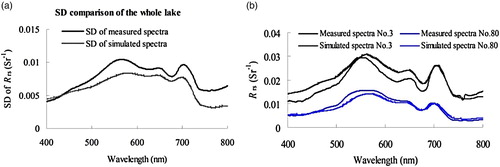
At sites No. 3 and No. 80, taken as two typical sites (refer to Table 1), the spectral shapes of the simulated and measured R_rs(λ) are compared (Fig. 3b). There is a satisfactory match between the simulation and measurement, particularly at longer wavelengths. A slight discrepancy exists around 570 nm and 700 nm. This error might arise from the following: the optical factor f/Q varies slightly from site to site but was taken as a constant for the entire lake; the simulated backscattering spectra were calculated from b_b(λ) at only seven wavelength bands. Besides, because of the unstable water conditions and subjective operations, instrument noise very likely existed when backscattering, remote-sensing reflectance, and even the absorption spectra were measured in the laboratory. Moreover, factors, such as skylight reflection, white caps on the water surface, and air–water interface reflectance, may all potentially cause errors (Li et al., 2010; Zhang et al., 2009a). On the other hand, it is noted that the effect of vegetation on the spectra is different, and the effect is stronger in the near-infrared and decreases with depth when compared with the spectra of sites No. 3 and No 80.

Nonetheless, the simulated R_rs(λ) can be taken as reliable because there is no great deviation in shape, magnitude, or other spectral features. In the following we examine the magnitudes and positions of the two typical peaks around 570 and 700 nm.

ii Peak magnitudes around 560 nm and 700 nm

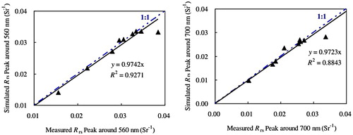
The remote-sensing reflectance spectra have two typical reflectance peaks around 560 and 700 nm. The 560 nm peak is attributed to chlorophyll and carotenoid absorption, as well as cell scattering; its peak magnitude depends on the pigment composition. The 700 nm peak is the most noticeable spectral feature of water with algae; it is defined as the fluorescence peak of chl a. The position and magnitude of this peak are indices for the estimation of chl a concentration. The magnitudes of the two peaks of the simulated R_rs(λ) and measured R_rs(λ) were compared site by site at the nine selected sites (Table 1). There are good matches between measured and simulated peak magnitudes around both 560 nm and 700 nm (see Fig. 4). The simulated versus measured values at the nine sites with different chl a concentrations are close to the 1:1 line, the slopes being 0.974 and 0.972 with high coefficients of determination R² of 0.93 and 0.88, respectively.

Fig. 4 Comparison of the peak magnitudes between the simulated R_rs(λ) and measured R_rs(λ) (left: first peak around 560 nm; right: second peak around 700 nm). The triangles indicate the simulated values; the dashed-dotted lines show y = x, and the solid lines show the actual relationship between the simulated and measured values.

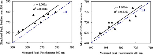
iii Peak positions around 560 nm and 700 nm

Besides magnitudes, the peak positions were also compared as shown in Fig. 5. Along with increasing chl a concentration, the positions of the reflectance peak around both 560 nm and 700 nm shift to longer wavelengths. Besides chl a, the positions are also affected by other water components, such as TSS. Thus, the peak positions might appear slightly irregular. It can be clearly seen from Fig. 5, that the positions of the simulated spectra and measured spectra have similar trends at around both 560 nm and 700 nm, and their peak positions are close to the 1:1 line (the slopes are 1.009 and 1.002, respectively).

Fig. 5 Comparison of the peak positions between the simulated R_rs(λ) and measured R_rs(λ) (left: first peak around 560 nm; right: second peak around 700 nm). The triangles indicate the simulated values; the dashed-dotted lines show y = x, and the solid lines show the actual relationship between the simulated and measured values.

Similarly, the simulated R_rs(λ) and measured R_rs(λ) are consistent in shape, magnitude, and reflectance. Table 2 provides the details of the comparison results at the nine selected sites. It can be concluded that the simulated R_rs(λ) spectra are reliable using the laboratory-analyzed data for the absorption and backscattering coefficients. Comparison of the simulated and measured R_rs(λ) allows us to estimate the contributions to the remote-sensing reflectance of the lake bottom and aquatic plants.

Table 2. Detailed description of the simulated and measured R_rs(λ) at the nine selected sites.

Sites	3	4	63	70	80	85	87	97	100
Measured Rrs(λ)
Peak_550 value (Sr^−1)	0.029	0.033	0.035	0.033	0.016	0.022	0.031	0.028	0.038
Peak_550 position (nm)	554	564	569	579	557	574	571	565	558
Peak_700 value (Sr^−1)	0.026	0.025	0.021	0.027	0.010	0.018	0.026	0.018	0.034
Peak_700 position (nm)	704	698	693	703	697	699	696	696	705
Simulated Rrs(λ)
Peak_550 value (Sr^−1)	0.031	0.033	0.034	0.034	0.014	0.022	0.031	0.027	0.033
Peak_550 position (nm)	561	577	570	580	563	578	576	569	565
Peak_700 value (Sr^−1)	0.026	0.025	0.023	0.027	0.010	0.017	0.027	0.018	0.028
Peak_700 position (nm)	707	697	695	701	700	700	698	700	703

3 Analysis of remote-sensing reflectance in OSWs

a Spectral Properties in OSWs

Four factors that can influence the spectra at the measuring sites are considered, namely, water depth, SDD transparency, chl a concentration, and aquatic plant status. To evaluate the contributions from the bottom and aquatic plants, several typical sites were selected for analysis using the following criteria: (i) different depth; (ii) different SDD and chl a; and (iii) different aquatic plant coverage. Other factors that can have an effect that are not mentioned in (i), (ii), or (iii) were similar at each of the selected sites.

1 different water depth, sdd, and chl a

From the perspective of water depth, sites No.51, 53, 54, and 57 with depths of 1.4, 1.5, 1.7, and 1.9 m, respectively, were selected to analyze the bottom contribution. None of the four sites had aquatic plants, and chl a concentration was approximately 10 mg m⁻³. Comparison of the spectra at the four sites showed that R_rs values in each of the wavelength bands increased as water depth decreased (Fig. 6a), indicating that the bottom mud in the OSWs of Lake Taihu has an obvious influence on R_rs spectra and the weighting becomes stronger if the water depth becomes shallower.

Fig. 6 (a) R_rs spectra measured at several typical sites with (a) different water depths (1.4, 1.5, 1.7, and 1.9 m) and (b) different SDD transparency (SDD = 0.7, 0.9, 1.375, and 1.75 m).

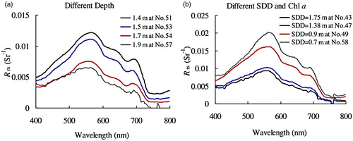
In comparison, SDD transparency reveals the opposite relationship to depth. Figure 6b gives the measured R_rs at the four typical sites where SDD transparency and chl a concentration differ. Because both TSS and phytoplankton pigment can affect SDD, SDD also influences R_rs spectra. Water depths at the four selected sites were approximately 2–2.1 m. Figure 6b clearly shows that the spectral values decrease as SDD values increase. This phenomenon is understandable because reflectance is usually higher in turbid water than clear water.

In addition to water depth and transparency, the number of aquatic plants in the OSWs was analyzed as the factor of most concern. The aquatic plants in the OSWs were mainly submerged, except for several sites where they grew to near the surface. From the records during the cruise, sites with two different distribution types of aquatic plants were used.

2 different heights of submerged plants

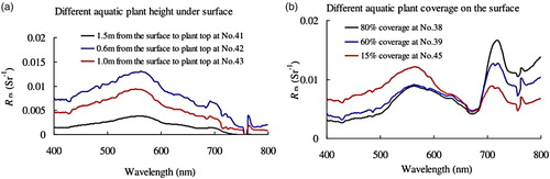
Three typical sites, where the aquatic plants were under the surface but reached different heights, were selected for this category. At sites No. 41, 42, and 43, the water depths and SDDs were almost the same even though the depth of the top of the aquatic plants varied, reaching 1.5, 0.6, and 1.0 m, respectively. Hence, we selected these three sites to compare the reflectance spectra, as shown in Fig. 7a. The influence of aquatic plants on the spectra varies considerably as the height changes. The closer the plant top was to the surface, the greater the contribution of aquatic plants to the reflectance spectra. However, though the aquatic plants existed under the water at the sampling sites, the reflectance spectra did not show much typical vegetation spectral properties in the near-infrared range, probably due to the absorption of energy reflected at these wavelengths by the water.

Fig. 7 (a) R_rs spectra measured at three typical sites with different aquatic plant heights under the water surface (0.6, 1.0, and 1.5 m from the surface to the aquatic plant top). (b) R_rs spectra measured at three typical sites with different percentages of aquatic plant cover on the water surface (15%, 60%, and 80% cover).

3 different percentage coverage of aquatic plants on the surface

Three sites were found in the OSWs where the aquatic plants reached very close to the water’s surface, and some of the leaves were floating on the surface. An estimate of the percentage of the sample site covered by floating leaves was recorded during the cruise (e.g., at sites No. 38, 39, and 45; the percentage covered was 80%, 60%, and 15%, respectively). They were notably different from the spectral properties described for aquatic plants. The R_rs spectra at the three sites showed strong vegetation information especially in the near-infrared range (see 680–800 nm in Fig. 7b, where the reflectance values are higher than those of the normal water spectrum). According to the percentage cover of aquatic plants, the R_rs values decrease in the visible band and increase in the near-infrared range with increasing percentage of vegetation cover. Among the spectra at the three sites, the difference was greatest around 710 nm and 400–600 nm, whereas the three spectra curves were extremely close in the of 610–700 nm range.

We also analyzed the measured R_rs spectra properties in the OSWs, which have different aquatic and bottom features. Comparison of these spectra can provide a general view of how aquatic plants and the bottom affect the remotely sensed reflectance. However, guaranteeing that the water types at all sites are similar is impossible, so comparisons from different sites, even with similar features, are not sufficiently rigorous for a reliable estimate of the contribution of bottom effects. One commonly used method is the simulation method of Lee et al. (1999) and others (Strombeck & Pierson, 2001), but a deficiency in the Hydrolight software sets a limitation for our present work.

b Contribution from Aquatic Plants and the Bottom

A computation method for the simulation of the R_rs spectra relies on the radiative transfer equations and the supporting data including optical factors Q and f, as well as absorption and backscattering coefficients from laboratory measurements. After careful analysis, the simulated R_rs spectra proved to be reliable. Therefore, the simulated R_rs spectra in the OSWs were utilized to compare with the measured R_rs and generate an approximate estimate of contribution rates of aquatic plants to the reflectance spectra.

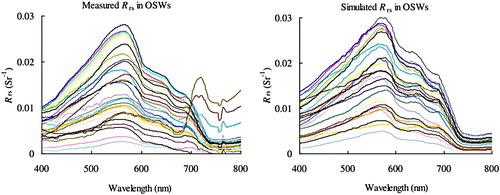
Among the 30 sites in the OSWs, simulated R_rs values were successfully obtained at only 28 sites because of a lack of backscattering measurements at sites No. 31 and No. 38. The measured and simulated R_rs spectra in OSWs are shown in Fig. 8. Based on cruise records, typical sites in the aquatic plant areas were selected to estimate the contribution of aquatic plants to the spectra.

Fig. 8 Measured R_rs spectra (left) and simulated R_rs spectra (right) in the OSWs of Lake Taihu.

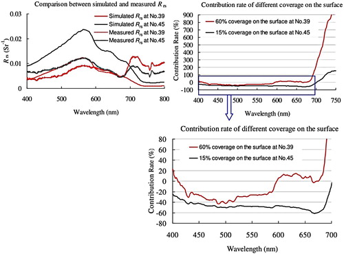
The contribution rates of aquatic plants to remote-sensing reflectance were estimated for the two different plant types mentioned above. For the case of those aquatic plants that grew to the surface, sites No. 39 and No. 45 with floating leaf vegetation coverage percentages of 60% and 15%, respectively, were selected. The simulated and measured R_rs spectra at the two sites were plotted in Fig. 9 (upper left), showing that the values for the simulated spectra were higher than for the measured spectra in the visible light region (400–700 nm). In contrast, in the near-infrared region, the simulated values continued to decrease while the measured spectra increased dramatically. With respect to magnitude, it is possible that the simulated R_rs spectrum at site No. 39 showed a lower value than that at site No. 45 because of the higher chl a concentration and lower SDD at site No. 45. The contribution rates of aquatic plants were also calculated for the two sites and are plotted in Fig. 9 (upper right and bottom right). At site No. 39, with 60% coverage of aquatic plants, the contribution rates in the 400–600 nm interval were mostly negative (from −40% to 0), but after the absorption dip around 675 nm, the aquatic plants contributed positively to the reflectance spectra, which increased sharply with wavelength. Nevertheless, at site No. 45 with 15% coverage, the contribution was negative, in the of 400–700 nm range but became positive after 700 nm. By comparing the two sites, we see that the aquatic plants at site No. 39 contributed to the reflectance in the near-infrared region much more than at site No. 45, but the negative contribution was smaller in the visible light region.

Fig. 9 Comparison of the simulated and measured R_rs (upper left) at sites No. 39 and No. 45 (two typical sites with different aquatic plant leaf cover floating on the surface) and the contribution rate estimate at the two sites from 400 to 750 nm (upper right) and magnified in the range of 400 to 700 nm (bottom right).

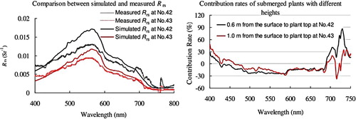
Of those sites where aquatic plants live under the surface but reach different depths below the surface, sites No. 42 and No. 43 were selected for the analysis. The distances from the water surface down to the top of the plants were 0.6 m and 1.0 m, respectively. Figure 10 (left) gives a comparison of the simulated and measured spectra at the two sites, showing that the simulated values of R_rs were higher than those for the measured R_rs for almost the entire 400–800 nm range. However, though aquatic plants are submerged in the water, they still wield an obvious influence on measured spectra, especially in the near-infrared region. The closer the plant tops were to the surface, the stronger the influence. For example, the aquatic plants at site No. 42 had a larger effect on the spectra than that at site No. 43. Figure 10 (right) shows the calculated contribution rates at the two sites. The contribution rates were negative (from zero to approximately −30%) in the of 420–680 nm range for site No. 42 and in the of 470–680 nm range for site No. 43; the influence was greater at site No. 42 than at site No. 43 in the 450–560 nm range, and little difference appeared in the 580–680 nm range. It is noteworthy that, beyond the pigment absorption minimum around 675 nm, the contribution becomes positive but weaker if the distance between the water surface and the plant tops is larger. Although some data scatter exists when estimating the contribution rates, the overall trends were still reasonable. Compared with the floating leaf vegetation type, the contribution of submerged plants to R_rs spectra was also considerably reduced over the entire wavelength band.

Fig. 10 Comparison of the simulated and measured R_rs (left) at sites No. 42 and No. 43 (two typical sites with different heights of submerged plants) and the contribution rate estimate at the two sites from 400 to 750 nm.

In the study, data validation of the results was carried out using the sub-dataset from the in situ data measured at about 30 sites in the OSWs of Lake Taihu in October 2008. In particular, we analyzed the spectra at different sites, categorized them into several water types, and compared the measured R_rs with the simulated R_rs spectra. The results were then compared with those of Ma et al. (2008) and also compared with the measurements from October 2010 (Duan et al., 2012). The comparison shows that they agree well in the distribution of aquatic plants in the eastern lake area.

4 Summary

In OSWs, the influence of the lake bottom and aquatic plants on the reflectance spectra was estimated using measured and simulated remote-sensing reflectance spectra at several sites that were different in depth and SDD value, as well as in aquatic plant growth and coverage. The simulated R_rs obtained from the measured absorption and backscattering spectra using radiative transfer theories proved to be reliable for further use after a careful comparison with different aspects of the measured spectra. Because the simulated R_rs in the OSWs is not significantly influenced by either aquatic plants or the lake bottom, it is valid to compare the simulated R_rs with the measured R_rs, and then approximate the contributions of aquatic plants and lake bottom to the remote-sensing reflectance in OSWs, such as Lake Taihu.

The influence of the various factors on spectra was analyzed from two aspects. One was to compare the spectral properties of the measured spectra using different characteristics (i.e., (i) different depth; (ii) different SDD and chl a, and (iii) different aquatic plant coverage). The other was to calculate the approximate contribution rates of aquatic plants by comparing the measured and simulated R_rs at selected typical sites. When only water depth was considered, the bottom mud in the OSWs of Lake Taihu had an obvious influence on R_rs spectra, and this influence grew even stronger as the water depth became shallower. The SDD transparency of the water revealed a reverse relationship. As far as the aquatic plants’ distribution was concerned, the closer the top of the aquatic plants was to the water surface, the higher the contribution of the aquatic plants to the reflectance spectra. According to the percentage cover of the aquatic plants, R_rs decreases in the visible wavelength range and increases in the near-infrared range as the percentage of vegetation cover increases. If the percentage cover of the aquatic plants on the water surface exceeds 60%, the remote-sensing reflectance shows similar spectral properties to terrestrial vegetation, especially in the red to near-infrared wavelengths. The simulated R_rs values were used to approximate the contribution rates from aquatic plants over the region of the visible and near-infrared wavelengths; the results showed an obvious positive contribution to the spectra at these wavelengths. As aquatic plant height or percentage cover increases so do the contribution rates.

Estimating the influence of aquatic plants on remote-sensing reflectance is the first and most important step towards the application of water colour remote sensing in complex shallow waters. The primary outcome of this investigation is of great significance for making useful calculations from future observations in these waters. It will help remove the influence of aquatic plants and lake bottom from the spectra and improve the accuracy of water colour parameter (especially chl a concentration) retrieval models in OSWs, such as Lake Taihu, China.

Disclosure statement

No potential conflict of interest was reported by the authors.

Additional information

Funding

This research was jointly supported by the National Key Research and Development Program of China [grant number 2016YFC1402003], the 2015 Innovation Program for Research and Entrepreneurship Teams, Jiangsu Province, China, and the Priority Academic Program Development of Jiangsu Higher Education Institutions (PAPD); 2015 Jiangsu Innovation Program.

References

- Albert, A., & Mobley, C. D. (2003). An analytical model for subsurface irradiance and remote sensing reflectance in deep and shallow case-2 waters. Optics Express, 11(22), 2873–2890. doi: 10.1364/OE.11.002873
- Buiteveld, H., Hakvoort, J. H. M., & Donze, M. (1994). The optical properties of pure water. Ocean Optics XII, SPIE, 2258, 174–183. doi: 10.1117/12.190060
- Ceyhun, Ö, & Yalcin, A. (2010). Remote sensing of water depths in shallow waters via artificial neural networks. Estuarine, Coastal and Shelf Science, 89, 89–96. doi: 10.1016/j.ecss.2010.05.015
- Clark, R. N. (1981). The spectral reflectance of water-mineral mixtures at low temperatures. Journal of Geophysical Research: Solid Earth, 86(B4), 3074–3086. doi: 10.1029/JB086iB04p03074
- Dekker, A. G., Vos, R. J., & Peters, S. W. M. (2001). Comparison of remote sensing data, model results and in situ data for total suspended matter (TSM) in the southern Frisian lakes. Science of the Total Environment, 268(1-3), 197–214. doi: 10.1016/S0048-9697(00)00679-3
- Duan, H., Loiselle, S. A., Zhu, L., Feng, L., Zhang, Y., & Ma, R. (2015). Distribution and incidence of algal blooms in Lake Taihu. Aquatic Sciences, 77, 9–16. doi: 10.1007/s00027-014-0367-2
- Duan, H., Ma, R., & Hu, C. (2012). Evaluation of remote sensing algorithms for cyanobacterial pigment retrievals during spring bloom formation in several lakes of east China. Remote Sensing of Environment, 126, 126–135. doi: 10.1016/j.rse.2012.08.011
- Gons, H. J. (1999). Optical teledetection of chlorophyll a in turbid inland waters. Environmental Science & Technology, 33(7), 1127–1132. doi: 10.1021/es9809657
- Gordon, H. R., Brown, O. B., & Jacobs, M. M. (1975). Computed relationships between the inherent and apparent optical properties of a flat homogeneous ocean. Applied Optics, 14, 417–427. doi: 10.1364/AO.14.000417
- Hedley, J. (2008). A three-dimensional radiative transfer model for shallow water environments. Optics Express, 16, 21887–21902. doi: 10.1364/OE.16.021887
- Hedley, J. D., Roelfsema, C. M., & Phinn, S. R. (2009). Efficient radiative transfer model inversion for remote sensing applications. Remote Sensing of Environment, 113, 2527–2532. doi: 10.1016/j.rse.2009.07.008
- Hedley, J. D., Roelfsema, C. M., Phinn, S. R., & Mumby, P. J. (2012). Environmental and sensor limitations in optical remote sensing of coral reefs: Implications for monitoring and sensor design. Remote Sensing, 4, 271–302. doi: 10.3390/rs4010271
- Henderson, R. K., Baker, A., Murphy, K. R., Hambly, A., Stuetz, R. M., & Khan, S. J. (2009). Fluorescence as a potential monitoring tool for recycled water systems: A review. Water Research, 43(4), 863–881. doi: 10.1016/j.watres.2008.11.027
- HOBI-labs Inc. (2008). Backscattering Sensor Calibration manual (Revision J). Retrieved from http://www.hobilabs.com
- Jiang, X., Jin, X., Yao, Y., Li, L., & Wu, F. (2008). Effects of biological activity, light, temperature and oxygen on phosphorus release processes at the sediment and water interface of Taihu Lake, China. Water Research, 42(8–9), 2251–2259. doi: 10.1016/j.watres.2007.12.003
- Kirk, J. T. O. (1994). Light and photosynthesis in aquatic ecosystems. Cambridge, UK: Cambridge University Press.
- Koponen, S., Pulliainen, J., Servomaa, H., Zhang, Y., Hallikainen, M., Kallio, K., … Hannonen, T. (2001). Analysis on the feasibility of multi-source remote sensing observations for chl-a monitoring in Finnish lakes. Science of the Total Environment, 268(1–3), 95–106. doi: 10.1016/S0048-9697(00)00689-6
- Lee, Z. P., & Carder, K. L. (2005). Hyperspectral remote sensing. In R. L. Miller, C. E. Del Castillo, & B. A. Mckee (Eds.), Remote sensing of coastal aquatic environments ( Ch. 8, pp. 181–204). Netherlands: Springer.
- Lee, Z. P., Carder, K. L., Mobley, C. D., Steward, R. G., & Patch, J. S. (1999). Hyperspectral remote sensing for shallow waters: 2 Deriving bottom depths and water properties by optimization. Applied Optics, 38, 3831–3843. doi: 10.1364/AO.38.003831
- Lee, Z. P., Carder, K. L., Mobley, C. D., Steward, R. G., Patch, J. S., & Gentili, B. (1998). Hyperspectral remote sensing for shallow waters I A semianalytical model. Applied Optics, 37, 6329–6338. doi: 10.1364/AO.37.006329
- Li, K., Liu, Z., & Gu, B. (2010). The fate of cyanobacterial blooms in vegetated and unvegetated sediments of a shallow eutrophic lake: A stable isotope tracer study. Water Research, 44(5), 1591–1597. doi: 10.1016/j.watres.2009.11.007
- Liu, X., Zhang, Y., Shi, K., Zhou, Y., Tang, X., Zhu, G., & Qin, B. (2015). Mapping aquatic vegetation in a large, shallow eutrophic lake: A frequency-based approach using multiple years of MODIS data. Remote Sensing, 7, 10295–10320. doi: 10.3390/rs70810295
- Lodhi, M. A., & Rundquist, D. C. (2001). A spectral analysis of bottom-induced variation in the colour of Sand Hills Lakes, Nebraska, USA. International Journal of Remote Sensing, 22(9), 1665–1682. doi: 10.1080/01431160117495
- Luo, J., Li, X., Ma, R., Li, F., Duan, H., Hu, W., … Huang, W. (2016). Applying remote sensing techniques to monitoring seasonal and interannual changes of aquatic vegetation in Taihu Lake, China. Ecological Indicators, 60, 503–513. doi: 10.1016/j.ecolind.2015.07.029
- Ma, R., & Dai, J. (2005). Quantitative estimation of chlorophyll-a and total suspended matter concentration with landsat ETM on field spectral features of Lake Taihu, Journal of Lake Sciences, 17(2), 97–103. doi: 10.18307/2005.0201
- Ma, R., Duan, H., Zhang, S., & Pan, D. (2008). Contribution of vegetation bottom to remote sensing reflectance in Taihu Lake, China [in Chinese]. Journal of Remote Sensing, 12(3), 483–489.
- Ma, R., Tang, J., & Dai, J. (2006). Bio-optical model with optimal parameter suitable for Taihu Lake in water colour remote sensing. International Journal of Remote Sensing, 27(19), 4305–4328. doi: 10.1080/01431160600857428
- Maritorena, S., Morel, A., & Gentili, B. (1994). Diffuse reflectance of oceanic shallow waters: Influence of water depth and bottom albedo. Limnology and Oceanography, 39, 1689–1703. doi: 10.4319/lo.1994.39.7.1689
- Mitchell, B. G. (1990). Algorithms for determining the absorption coefficient of aquatic particulates using the quantitative filter technique (QFT). Ocean Optics X. SPIE, 1302, 137–148. doi: 10.1117/12.21440
- Mobley, C. D. (1994). Light and water: Radiative transfer in natural waters. New York: Academic Press.
- Morel, A., & Gentili, B. (1993). Diffuse reflectance of oceanic waters. II Bidirectional aspects. Applied Optics, 32, 6864–6879. doi: 10.1364/AO.32.006864
- Mueller, J. L., Fargion, G. S., & McClain, C. R. (2003). Ocean optics protocols for satellite ocean color sensor validation ( Revision 4, Vols 1–4). Maryland: Greenbelt.
- Pope, R. M., & Fry, E. S. (1997). Absorption spectrum (380–700 nm) of pure water. II Integrating cavity measurements. Applied Optics, 36, 8710–8723. doi: 10.1364/AO.36.008710
- Pulliainen, J., Kallio, K., Eloheimo, K., Koponen, S., Servomaa, H., Hannonen, T., … Hallikainen, M. (2001). A semi-operative approach to lake water quality retrieval from remote sensing data. Science of the Total Environment, 268(1–3), 79–93. doi: 10.1016/S0048-9697(00)00687-2
- Qin, B., Hu, W., & Chen, W. (2004). Evolvement process and mechanism of water environment in Taihu Lake. Beijing: Science Press. (in Chinese).
- Ritchie, J., & Cooper, C. (1991). An algorithm for estimating surface suspended sediment concentrations with Landsat MSS digital data. Water Resources Research, 27, 373–379.
- Shi, K., Zhang, Y., Zhu, G., Liu, X., Zhou, Y., Xu, H., … Li, Y. (2015). Long-term remote monitoring of total suspended matter concentration in Lake Taihu using 250 m MODIS-aqua data. Remote Sensing of Environment, 164, 43–56. doi: 10.1016/j.rse.2015.02.029
- Smith, R. C., & Baker, K. S. (1981). Optical properties of the clearest natural waters (200–800 nm). Applied Optics, 20, 177–184. doi: 10.1364/AO.20.000177
- Strombeck, N., & Pierson, D. C. (2001). The effects of variability in the inherent optical properties on estimations of chlorophyll a by remote sensing in Swedish freshwaters. Science of the Total Environment, 268(1–3), 123–137. doi: 10.1016/S0048-9697(00)00681-1
- Wang, H. (1985). The water resources of lakes in China. GeoJournal, 10(2), 151–155. doi: 10.1007/BF00150733
- Woźniak, B., Dera, J., Ficek, D., Majchrowski, R., Kaczmarek, S., Ostrowska, M., & Koblentz-Mishke, O. I. (1999). Modelling the influence of acclimation on the absorption properties of marine phytoplankton. Oceanologia, 41(2), 187–210.
- Woźniak, B., Woźniak, S. B., Tyszka, K., Ostrawska, M., Majchrowski, R., Ficek, D., & Dera, J. (2005). Modelling the light absorption properties of particulate matter forming organic particles suspended in seawater. Part 2. Modelling Results. Oceanologia, 47, 621–662.
- Yentsch, C. S. (1962). Measurement of visible light absorption by particulate matter in the ocean. Limnology and Oceanography, 7, 207–217. doi: 10.4319/lo.1962.7.2.0207
- Zhang, Y., Liu, M., Qin, B., van der Woerd, H. J., Li, J., & Li, Y. (2009a). Modeling remote-sensing reflectance and retrieving chlorophyll-a concentration in extremely turbid case-2 waters (Lake Taihu, China). IEEE Transactions on Geoscience and Remote Sensing, 47(7), 1937–1948. doi: 10.1109/TGRS.2008.2011892
- Zhang, Y., van Dijk, M. A., Liu, M., Zhu, G., & Qin, B. (2009b). The contribution of phytoplankton degradation to chromophoric dissolved organic matter (CDOM) in eutrophic shallow lakes: Field and experimental evidence. Water Research, 43(18), 4685–4697. doi: 10.1016/j.watres.2009.07.024