Uncertainty of the Linear Trend in the Zonal SST Gradient Across the Equatorial Pacific Since 1881

ABSTRACT

The change in the zonal sea surface temperature gradient (ZSSTG) across the equatorial Pacific plays an important role in the global climate system. However, there has not yet been a consensual conclusion about the changing ZSSTG at either a short-term (from 20 to 90 years) or a long-term time scale (longer than 90 years) in the literature. In this study, the uncertainty of the trend in ZSSTG for different sub-periods since 1881 was examined using four interpolated datasets and four un-interpolated datasets. It was found that the trend in ZSSTG on the short-term time scale could be significantly influenced by internal variability such as the El Niño–Southern Oscillation and the Pacific Decadal Oscillation. On the long-term time scale, the sign of the ZSSTG trend depends on the dataset used. In particular, it was not possible to draw a uniform conclusion about the secular trends in ZSSTG in recent history, given the high sensitivity of the ZSSTG trends to the period, dataset, and regions used to calculate the trends. Our results imply that it may not be possible to detect the response of ZSSTG to global warming until a longer data record becomes available in the future.

RÉSUMÉ

[Traduit par la rédaction] La modification du gradient zonal de la température de la surface de la mer (SST) dans le Pacifique équatorial influe grandement sur le système climatique mondial. Cependant, il n’y a toujours pas de consensus dans la littérature en ce qui a trait à l’échelle temporelle de ces changements: court terme (de 20 à 90 ans) ou long terme (plus de 90 ans). Dans cette étude, nous examinons l’incertitude de la tendance du gradient zonal des SST pour diverses sous-périodes depuis 1881, et ce, en utilisant quatre ensembles de données interpolées et quatre ensembles de données non interpolées. Nous avons constaté que la tendance à court terme du gradient zonal des SST pourrait être fortement régie par des variations internes, comme le phénomène El Niño-oscillation australe et l’oscillation décennale du Pacifique. À long terme, le signe de la tendance du gradient zonal des SST dépend de l’ensemble de données utilisé. Notamment, nous ne pouvons tirer de conclusion cohérente sur les tendances séculaires récentes du gradient zonal des SST, étant donné la grande sensibilité des tendances de ce gradient relativement à la période, aux données et aux régions utilisées pour calculer les tendances. Nos résultats indiquent qu’il ne sera peut-être pas possible de détecter la réaction du gradient zonal des SST que produirait le réchauffement de la planète, tant qu’il n’existera pas une série plus longue de données.

KEYWORDS:

• trend
• zonal SST gradient
• data inconsistency
• uncertainty

1  Introduction

The zonal sea surface temperature gradient (ZSSTG) in the equatorial Pacific Ocean, represented by the regional averaged sea surface temperature (SST) difference between the eastern equatorial Pacific and the western equatorial Pacific (Karnauskas, Seager, Kaplan, Kushnir, & Cane, 2009; Sandeep, Stordal, Sardeshmukh, & Compo, 2014), is a defining feature of the climate system. It is closely coupled to the Walker Circulation (Tokinaga, Xie, Deser, Kosaka, & Okumura, 2012) and can interact strongly with the dominant internal variability, such as an El Niño–Southern Oscillation (ENSO) event (Clement, Seager, Cane, & Zebiak, 1996). The study of long-term changes in ZSSTG can advance our understanding of how the climate system responded to anthropogenic greenhouse gas (GHG) forcing in history. Although progress has been made in explaining mechanisms behind the changing ZSSTG under GHG forcing, the question remains as to whether the ZSSTG has been strengthened or weakened in recent history.

The long-term change in the ZSSTG is primarily associated with two mechanisms. The “ocean thermostat” mechanism implies that under uniform heating in the tropical Pacific, the heat input to the eastern equatorial Pacific Ocean would be largely compensated for by enhanced upwelling there because of increased surface-layer stratification. The ZSSTG in this case is expected to be enhanced (Cane et al., 1997; Clement et al., 1996). In contrast, model and theoretical studies suggest that the tropical atmospheric circulation and hydrological cycle should weaken in response to anthropogenic GHG forcing (Held & Soden, 2006; Vecchi et al., 2006; Xie et al., 2010), resulting in a slowdown of the Walker Circulation and a further reduction in the ZSSTG. These two competing mechanisms imply opposite changes in the ZSSTG under global warming.

Interestingly, both mechanisms can be verified by using different datasets of the recent history. Using the interpolated datasets, many studies reported that the twentieth century SST trend was negative in the eastern equatorial Pacific and was positive in the western equatorial Pacific, implying that the ZSSTG strengthened in the past century (e.g., Cane et al., 1997; Clement et al., 1996; Karnauskas et al., 2009) However, Deser, Phillips, and Alexander (2010) argued that the in situ measurements in the eastern equatorial Pacific were poor, and the SST trend estimated by the interpolated datasets thus cannot be fully trusted. Instead, using the un-interpolated datasets, Deser et al. found that the eastern equatorial Pacific was warmer than the western equatorial Pacific in the twentieth century indicating that the ZSSTG had weakened in the twentieth century. These findings suggest that the sign of the secular trend in ZSSTG over the past century depends on whether the dataset used is interpolated or un-interpolated.

Even for the same dataset, different conclusions about the ZSSTG trend may be drawn when different periods are used in calculating the trend. For example, using the Extended Reconstructed SST, version 3 (ERSST3; Smith, Reynolds, Peterson, & Lawrimore, 2008), Karnauskas et al. (2009) found that the ZSSTG intensified during the 1880–2005 period. On the contrary, Deser et al. (2010) concluded that the ZSSTG weakened by using the same dataset but with a different period (1900–2010). The sensitivity of the ZSSTG trend to the period used may be caused by strong interannual variability, such as ENSO, in the time series (L’Heureux, Collins, & Hu, 2012), but it is not yet clear how much or for how long ENSO events can affect the ZSSTG trend. In addition, L’Heureux, Lee, and Lyon (2013) argued that the SST trend in the eastern equatorial Pacific had a strong decadal variation. Whether the ZSSTG trend also contains such a decadal variation or the physics that would be behind this decadal variation have not yet been addressed.

Finally, the equatorial area used to define the ZSSTG may introduce uncertainty in the ZSSTG trend. Generally, the equatorial area overlapping the warm pool and cold tongue can be used to define the ZSSTG, but there has been no agreement on which regions should be used (L’Heureux et al., 2012; Sandeep et al., 2014; Tokinaga et al., 2012). To our knowledge, the sensitivity of the ZSSTG trend to the area used in the trend estimation has not been discussed in previous works.

In this study, the uncertainty of the linear trend in the ZSSTG related to the period, dataset, and regions used to estimate the trend is investigated using four interpolated datasets and four un-interpolated datasets. In particular, we explore the effects of the dominant climate modes in the Pacific on the ZSSTG trend. Our aims are to quantify how large the uncertainty in the changing ZSSTG was in recent history and whether we can draw a uniform conclusion about the secular trends in ZSSTG using available datasets. The rest of the paper is arranged as follows. Data and method are described in Section 2. The uncertainty in the ZSSTG trend since 1881 is discussed in Section 3. In Section 4, we investigate the relationships between internal variability and the ZSSTG trend at short-term and long-term time scales. In Section 5, we discuss the uncertainty in the ZSSTG trend resulting from the data type used. In Section 6, we discuss the uncertainty in the ZSSTG trend associated with different equatorial regions used to define the ZSSTG. The ZSSTG trend during the past three decades is investigated in Section 7, followed by a discussion and conclusions in Section 8.

2  Data and method

Four sets of interpolated SST reconstructions and four sets of un-interpolated surface temperature archives are used in this study. The interpolated datasets include the monthly-mean Hadley Centre sea ice and SST, version 1 (HadISST1; Rayner et al., 2003), Kaplan SST, version 2 (Kaplan2; Kaplan et al., 1998), ERSST3, and the Centennial in Situ Observation Based Estimates of SST (COBE2; Ishii, Shouji, Sugimoto, & Matsumoto, 2005) reconstructions. The un-interpolated datasets include the monthly-mean Hadley Centre/Climate Research Unit Temperature, version 3, variance-adjusted (HadCRUT3; Brohan, Kennedy, Harris, Tett, & Jones, 2005), HadCRUT4 (Morice, Kennedy, Rayner, & Jones, 2012), Merged Land-Ocean Surface Temperature Analysis (MLOST3.5; Smith et al., 2008), and Goddard Institute for Space Studies (GISS; Hansen, Ruedy, Sato, & Lo, 2010) archives. These un-interpolated archives include both SST and land surface temperature data, but we will simply call them SST datasets hereafter for convenience. The period, resolution, and type of the datasets are listed in Table 1. The period used in this study is 1881–2013. The climatological seasonal cycle is removed from all datasets prior to analysis.

Table 1. A brief description of the datasets used in this study.

Name	Period	Resolution	Type
HadISST1	1870–2013	1.0° × 1.0°	Interpolated
Kaplan2	1856–2013	5.0° × 5.0°	Interpolated
ERSST3	1854–2013	2.0° × 1.0°	Interpolated
COBE2	1850–2013	1.0° × 1.0°	Interpolated
HadCRUT3	1850–2013	5.0° × 5.0°	Un-interpolated
HadCRUT4	1850–2013	5.0° × 5.0°	Un-interpolated
MLOST3.5	1880–2013	5.0° × 5.0°	Un-interpolated
GISS	1880–2013	2.0° × 1.0°	Un-interpolated

The ZSSTG is defined as the difference in the area-averaged SST anomaly between the eastern equatorial Pacific (5°S–5°N, 150°W–90°W, or the Niño 3 region) and the western equatorial Pacific (5°S–5°N, 120°E–180°), namely, the anomaly in the east minus that in the west. The least-squares method is used to estimate the linear trend coefficients for different periods. Because the climatological SST in the eastern equatorial Pacific is colder than that in the western equatorial Pacific zone a negative (positive) linear regression coefficient of the ZSSTG means a strengthening (weakening) trend. Following Deser et al. (2010), we only consider the grids that have at least three samples per decade in estimating trend from the un-interpolated datasets.

For a selected period, the trend estimated from a given dataset is regarded to be significant if it can pass the 95% confidence level (the Student’s t-test). Moreover, only significant trends are used to construct the multi-dataset–averaged ZSSTG trend for the given period. In particular, the trend in a given period is regarded to be robust only when all eight datasets uniformly exhibit a significant strengthening or weakening trend.

At the interannual time scale, the dominant mode in the tropical Pacific is ENSO, which can be expressed by the averaged SST anomaly in the Niño 3 region. Because the variation of the SST anomaly in the western equatorial Pacific is much less than that in the Niño 3 region, the ZSSTG index defined here can also, to a great extent, represent ENSO. At the decadal time scale, the dominant mode is the Pacific Decadal Oscillation (PDO; Mantua, Hare, Zhang, Wallace, & Francis, 1997). The PDO index is defined as the 10-year running mean of the leading principal component of the SST anomaly over the northern Pacific from 1900 to 2010. The short-term and long-term periods used in this study are defined as a duration of 20–90 years and a duration longer than 90 years, respectively.

3  Uncertainty in the ZSSTG trend since 1881

The ZSSTG trend depends heavily on the period and dataset in which the trend is estimated. As an example, Fig. 1 compares the 93-year SST trends in the tropical Pacific estimated from the HadISST1 and ERSST3 datasets during the 1908–2000 and 1911–2003 periods, respectively. Note that the 93-year duration was chosen arbitrarily. One can also use 90 or 100 years, or another long-term duration to compare trends, as will be shown later. During the 1908–2000 period, most areas of the Pacific Ocean exhibited warming trends (Figs 1a and 1b). However, in the eastern equatorial Pacific, the trend based on the HadISST1 dataset was negative, which is opposite to the trend based on the ERSST3 dataset. Consequently, using the ERSST3 dataset produces a weakening ZSSTG trend of 0.17°C per century, in contrast to a strengthening trend of −0.15°C per century produced using the HadISST1 dataset. Note that the negative ZSSTG trend estimated from HadISST1 in this case is statistically significant only at the 90% confidence level. Nevertheless, this example clearly illustrates that whether the ZSSTG is intensified or not depends heavily on the dataset used for the selected period.

Fig. 1 The linear trend in the tropical Pacific SST (°C per century) estimated using the HadISST1 (top panels) and ERSST3 (bottom panels) datasets during the 1908–2000 (left panels) and 1911–2003 (right panels) periods. The numbers at the top right denote the ZSSTG trend. Black boxes in (a) indicate the regions used to define the ZSSTG. Black dots indicate trends that pass the 95% significance test.

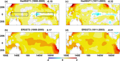
Shifting the period used to calculate the trend by merely three years (i.e., for the period from 1911 to 2003), we find that the general pattern of the SST anomaly trend does not change significantly. However, the trend in the eastern equatorial Pacific greatly decreases in both datasets. The negative trend is doubled for the HadISST1 dataset, up to −0.32°C per century, and is statistically significant at the 95% confidence level. For the ERSST3 dataset, the ZSSTG trend becomes a rather small negative value (−0.01°C per century) with no statistical significance, which is obviously different from the finding of the weakening ZSSTG using the 1908–2000 period.

It is thus necessary to explore the uncertainty in the ZSSTG trend as a function of the period used. Figure 2 presents the statistically significant trend in ZSSTGs in any sub-period since 1881 as a function of the start and end years based on ERSST3 data. We use two colours to indicate positive and negative values for clarity. The sign of the ZSSTG trend exhibits a strong decadal variation when the duration used to estimate the trend falls in the short-term time scale. For example, if the duration is fixed at 50 years, the trend is positive when the end year is earlier than the 1940s, indicating that the 50-year ZSSTG is weakened. When the end year is between 1941 and 1980, the trend is negative, suggesting that the 50-year ZSSTG is intensified. If the end year is set after the 1980s, the ZSSTG trend is again positive.

Fig. 2 The ZSSTG trend (°C per century) for different periods estimated using the ERSST3 dataset. The x- and y-axes denote the end year and start year of the period, respectively. Green lines indicate 20-year and 90-year durations, and the red line indicates a 50-year duration. Open black circles indicate the 1908–2000 and 1881–1998 periods. Open orange triangles indicate the 1895–1990 and 1900–2010 periods. The pink and cyan indicate positive and negative values, respectively. The two extreme El Niño events of 1982/83 and 1997/98 are marked.

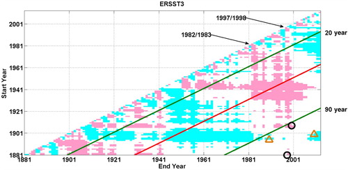
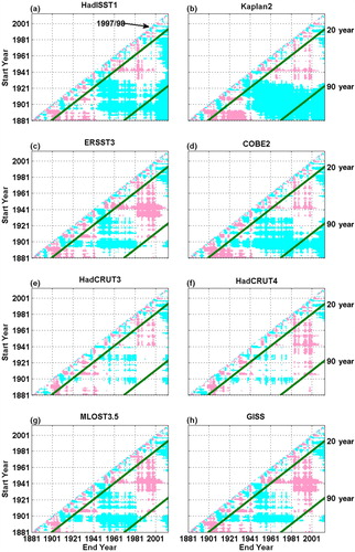
At the long-term time scale, the ZSSTG trend estimated from ERSST3 data is not significantly different from zero for most pairs of start and end years, although one may be able to choose a period to obtain a significant positive (around the 1908–2000 and 1881–1998 periods, open black circles) or negative (around the 1895–1990 and 1900–2010 periods, open orange triangles) trend. However, these significant trends estimated from ERSST3 data are not consistently demonstrated using the other seven datasets. Figure 3 gives the ZSSTG trend for all eight datasets. The decadal variation of the ZSSTG trend can be clearly seen in all the datasets when the duration falls in the short-term time scale. At the long-term time scale, the insignificant ZSSTG trend in most pairs of start and end years from the ERSST3 data can be supported by the four un-interpolated datasets, especially by the GISS dataset. However, from HadISST1, Kaplan2, and the COBE2 datasets, significant negative trend coefficients are found instead for most pairs of start and end years, implying an intensification of the ZSSTG. This example clearly shows that any conclusions about the ZSSTG trend for the long-term period depends heavily on the datasets used.

Fig. 3 The ZSSTG trend (°C per century) for different periods since 1881. Colours and lines are as in Fig. 2. The extreme El Niño event of 1997/98 is marked.

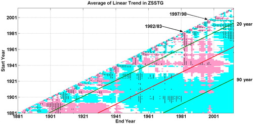
We then average the significant trends in each pair of start and end years to obtain a multi-dataset estimation of the ZSSTG trend in any sub-period since 1881. In Fig. 4, the periods during which all eight datasets uniformly exhibit a strengthening or weakening trend are marked with dots. These trends are regarded as the robust trends. As seen in Fig. 4, the multi-dataset average of ZSSTG trends also exhibits a strong decadal variation for the periods at the short-term time scale. However, only 6.61% of the pairs have a robust trend, indicating that there is a large uncertainty associated with the sign of the ZSSTG trend at this time scale because of the inconsistent representation of internal variability in the different datasets used (Tokinaga et al., 2012). The multi-dataset average of ZSSTG trends at the long-term time scale is negative, suggesting that the long-term change in the ZSSTG is strengthened. However, as shown in Fig. 3, this strengthened ZSSTG comes mainly from three of the interpolated datasets. When all eight datasets are considered, none of the ZSSTG trends is robust at the long-term time scale. In other words, one may arbitrarily choose a dataset to get a strengthened, weakened, or insignificant long-term change in the ZSSTG.

Fig. 4 The multi-dataset average of the ZSSTG trend. The pairs of years with robust trends are shown as dots. Colours and lines are as in Fig. 2. The two extreme El Niño events of 1982/83 and 1997/98 are marked.

4  Uncertainty in the ZSSTG trend resulting from internal variability

a  Uncertainty Associated with ENSO

Figure 2 suggests that the sign of the ZSSTG trend at the short-term time scale could be significantly influenced by ENSO, especially by extreme El Niño events (Chen et al., 2015; Hong, Ho, & Jin, 2014). For example, using 1961 as the start year, the ZSSTG trend estimated from ERSST3 data is not significant when the end year is earlier than 1982 (Fig. 2). When the end year is moved to 1983, which includes the extreme 1982/83 El Niño event, the ZSSTG trend suddenly becomes a significant positive value. When the end year is moved to 1984, the ZSSTG trend is again insignificant. The change in the sign of the ZSSTG trend can also be seen when the end year is near other strong El Niño episodes, such as 1997/98 (Fig. 2); this is true for all datasets (Fig. 3).

The reason the ZSSTG trend is so sensitive to El Niño is simply that the amplitude of ENSO is much greater than the magnitude of the ZSSTG trend (e.g., Sandeep et al., 2014). The variation of the SST anomaly in the western equatorial Pacific is relatively small; thus, by definition, the variation of the ZSSTG will depend heavily on the variation of the SST anomaly in the eastern equatorial Pacific. When a strong El Niño or La Niña occurs at the start or end of the period, it can change the sign of the ZSSTG trend. Such a strong influence of ENSO on the ZSSTG trend can last for many decades. As seen in Figs 2 and 3, even when the duration is longer than 90 years, the impact of El Niño on the ZSSTG trend can still be seen.

However, when the multi-dataset average of the ZSSTG trends is considered, the influence of strong ENSO events on the sign of the ZSSTG is no longer strong (Fig. 4), especially when the duration used is relatively long. This is mainly caused by the inconsistent representations of ENSO among the datasets (Solomon & Newman, 2012). For example, the influence of the 1997/98 extreme El Niño on the ZSSTG trend is much less for the HadISST1 dataset than for the ERSST3 one (Fig. 3). Thus, the trend during the period with end years around 1998 is robust only in a few pairs of start and end years (Fig. 4).

b  Uncertainty Associated with the PDO

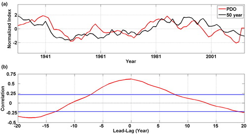
As discussed above, the ZSSTG trend at the short-term time scale exhibits a strong decadal variation. In the Pacific Ocean, the leading mode at the short-term time scale is the PDO (Mantua et al., 1997). The PDO is dominant in the North Pacific but also has a strong influence on the evolution of SST in the equatorial Pacific (Zhang, Wallace, & Battisti, 1997). Figure 5 shows the evolution of the 10-year running mean of the ZSSTG and the PDO index for the four interpolated datasets. It is clear that the low-frequency variation of the ZSSTG is closely related to the PDO. For all four interpolated datasets, the correlation coefficients between the 10-year running mean of the ZSSTG and PDO index are statistically significant at the 95% confidence level. Because of this, the variation of the 50-year ZSSTG trend is closely related to the PDO index, as shown in Fig. 6a. The maximum correlation occurs when the PDO index is in phase with the 50-year ZSSTG trend (Fig. 6b). This relationship between the PDO index and the 50-year ZSSTG trend can also be found in each of the interpolated datasets (not shown). We also used other durations at the short-term time scale and obtained comparably high correlations between the PDO and the ZSSTG trend (not shown), indicating that the PDO plays a fundamental role in changing the ZSSTG trend at a short-term time scale.

Fig. 5 The normalized 10-year running mean of the ZSSTG (blue line) and the normalized PDO index (red line) for the four interpolated datasets. The number at the top right of each panel is the correlation coefficient.

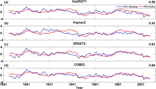
Fig. 6 (a) Evolution of the 50-year multi-dataset–averaged ZSSTG trend (black line) and the multi-dataset average of the PDO indices (red line) estimated using the interpolated datasets. (b) Lead-lag correlation of the two curves shown in (a). Solid blue lines indicate the 95% confidence interval. Negative (positive) numbers denote the 50-year multi-dataset–averaged ZSSTG trend leading (lagging) the PDO index.

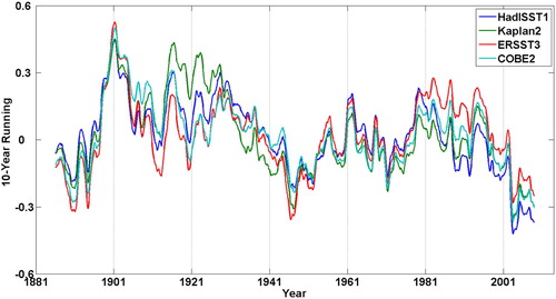
However, as with the discrepancy in the representation of ENSO among the different datasets, the projections of the PDO on the equatorial Pacific are also quite inconsistent in the interpolated datasets. Figure 7 compares the 10-year running mean of the ZSSTG among the four interpolated datasets. Although the evolution of the 10-year running mean of the ZSSTG is, in general, consistent among the datasets, there are two periods with distinct discrepancies. The first period is around 1920. In this period, the 10-year running mean of the ZSSTG from the Kaplan2 SSTs is much greater than for others. This explains why there are more pairs of years with significant negative trends from Kaplan2 when the start year is around 1920 and the end year is earlier than 1980 (Fig. 3). The second period is around 1990 when the ERSST3 dataset shows a stronger 10-year running mean for the ZSSTG than the other three datasets. As a result, more pairs of years with a significant positive ZSSTG trend are found using the ERSST3 data when the end year is around 1990 (Fig. 3). Summarizing the results shown in Fig. 7 and Fig. 3, we conclude that the discrepancies in the 10-year running mean of the ZSSTG among the datasets, which are highly related to the PDO, lead to the sparse pairs of years with robust ZSSTG trends at the short-term time scale shown in Fig. 4.

Fig. 7 The 10-year running mean of the ZSSTG for the four interpolated datasets.

5  Uncertainty associated with data type

In Sections 3 and 4, we found that the ZSSTG trend depends heavily on the type of dataset used, that is, whether the dataset is reconstructed or not. Deser et al. (2010) argued that the reconstruction procedure could lead to the poor data quality for the SSTs in the eastern equatorial Pacific. As a result, the sign of the ZSSTG trends estimated from the interpolated datasets strongly depends on the dataset used. On the other hand, the ZSSTG trends estimated from the un-interpolated datasets are negative, and these negative trends are very robust across different un-interpolated SST datasets (Deser et al., 2010; Tokinaga et al., 2012).

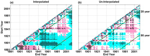
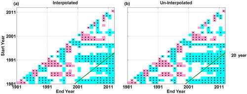
Figure 8 presents the ZSSTG trend in different periods using the interpolated and un-interpolated datasets. As can be seen, the decadal variation of the sign of the ZSSTG trend at the short-term time scale can be found in both types of datasets. At the long-term time scale, both interpolated and un-interpolated datasets give negative ZSSTG trends in many pairs of start and end years, but only 6.65% and 0.22% are robust for the interpolated and un-interpolated datasets, respectively. These results indicate that, unlike the argument of Deser et al. (2010), the trends from the un-interpolated datasets also depend heavily on the datasets used; thus, it is difficult to conclude that there is a robust secular trend in the ZSSTG using these un-interpolated datasets.

Fig. 8 As in Fig. 4, but for (a) the interpolated datasets and (b) the un-interpolated datasets.

6  Uncertainty associated with regions defining ZSSTG

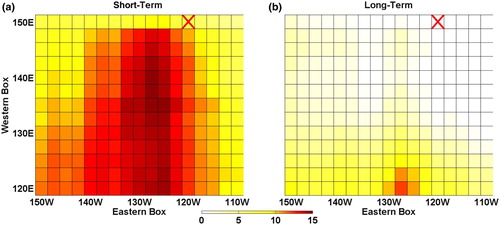
Figure 9 shows the percentage of pairs of start and end years that have robust trends as a function of the central longitudes used to define the western equatorial Pacific box and the eastern equatorial Pacific box associated with the ZSSTG. The regions used to define the ZSSTG in the previous sections are indicated with a red cross. At the short-term time scale, a high percentage is found when the eastern box is located around 125°W (Fig. 9a), leading to about 15% of the total pairs of start and end years having robust trends. At the long-term time scale, the maximum percentage is found when the western box is around 120°E and the eastern box is located around 130°W with 12% of the pairs of start and end years being robust (Fig. 9b). Nevertheless, these percentage values are still too small; thus, the large uncertainty in the secular trend of the ZSSTG discussed in previous sections should not be very dependent on the definition of the ZSSTG.

Fig. 9 The percentage of pairs of years that have a robust ZSSTG trend at (a) short-term and (b) long-term time scales as functions of the central longitudes of the western equatorial Pacific and the eastern equatorial Pacific. Red crosses indicate the central longitudes used to define the western equatorial Pacific and the eastern equatorial Pacific in this study.

7  ZSSTG trend during the past three decades

Recent studies have reported that the ZSSTG in the past three decades intensified significantly (England et al., 2014; McPhaden, Lee, & McClurg, 2011). This finding can be easily verified using our analysis method. Figure 10 shows the ZSSTG trend at each pair of start and end years since 1981 from the eight datasets. When the duration of the period is longer than 20 years, all eight datasets exhibit negative ZSSTG trends in most pairs of start and end years. More importantly, the ZSSTG trends for more than half the periods are robust (not shown). In addition, this robust strengthening trend can be found in both interpolated and un-interpolated datasets for more than half the total pairs of start and end years (Fig. 11), which does not depend on the definition of the ZSSTG (not shown).

Fig. 10 As in Fig. 3, but for the ZSSTG trend since 1981.

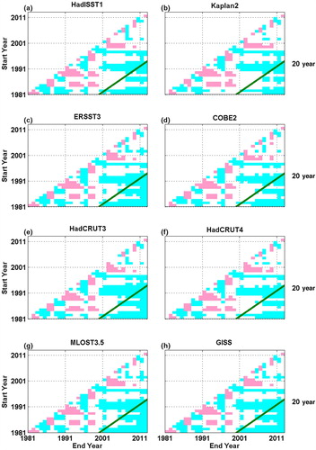
Fig. 11 As in Fig. 8, but for the ZSSTG trend since 1981.

8  Discussion and conclusions

In this study, the ZSSTG trend in each pair of start and end years since 1881 was investigated using four interpolated and four un-interpolated datasets. It is found that the ZSSTG trend depends heavily on the period and dataset used, as well as the regions in which the trend is estimated.

First, internal variability, such as ENSO and the PDO, exerts a strong influence on the ZSSTG trend. The ZSSTG trend shows a distinct decadal variation when the duration evaluated falls in the short-term time scale. This decadal variation is closely related to the projection of the PDO on the equatorial Pacific. Strong ENSO events could also significantly affect the ZSSTG trend. For some extreme El Niño events such as the 1982/83 and 1997/98 events, the sign of the ZSSTG trends can change suddenly if the start or end year is set to the extreme El Niño years, even when the trends are estimated using records that are nearly 100 years in length. Because anthropogenic forcing exists in any long time span from the Industrial Revolution onward, the strong sensitivity of the ZSSTG trend to the long-term period suggests that any statement about the ZSSTG change in history based on a single record (e.g., the twentieth century) should be interpreted with caution.

Second, the sign of the secular trend of the ZSSTG depends on the dataset used. Although some datasets suggest that the ZSSTG intensified over our period of interest (1881–2013), others imply that the ZSSTG has no significant trend or even weakened. The multi-dataset–averaged ZSSTG trends at the long-term time scale are negative, but only 6.61% of these negative long-term trends are supported by all the datasets. Unlike arguments in previous studies, we found that the secular ZSSTG trends estimated from the un-interpolated datasets also depend heavily on the datasets used; thus, it is difficult to conclude that there is a robust secular trend in ZSSTG using available datasets. However, for the trend during the past three decades, a negative ZSSTG trend can be uniformly obtained by all eight datasets, indicating that the recent intensification of the ZSSTG is a robust climate signal.

Last, the percentage of ZSSTG trends that can be uniformly obtained by all eight datasets is sensitive to the regions used to define the ZSSTG, yet the percentage is very low, in general. Based on these findings, we conclude that the ZSSTG trend is weak compared with internal variability and shows inconsistent representation among different datasets. Thus, one may not be able to detect the change in the ZSSTG until a longer data record becomes available in the future.

The large uncertainty in the ZSSTG trend resulting from the period used to estimate the trend can be attributed to the fact that the amplitude of the multi-scale internal variability is much larger than the magnitude of the ZSSTG trend (Sandeep et al., 2014). To alleviate such an influence, it is usually recommended that ENSO signals be removed before analyzing the ZSSTG trends in the tropical Pacific. For example, Cane et al. (1997) screened out the ENSO signal by removing the leading empirical orthogonal function mode of tropical Pacific SSTs from the data. Parker et al. (2007) applied a bandpass filter to raw data to remove the interannual SST signal. Compo and Sardeshmukh (2010) introduced a linear inverse model to separate SST records into an ENSO-related component and an ENSO-unrelated component. Solomon and Newman (2012) further applied the linear inverse model to different observational datasets and concluded that there are distinct cooling trends in the eastern equatorial Pacific and warming trends in the western equatorial Pacific when ENSO is removed from the datasets. Recently, Coats and Karnauskas (2017) applied the same method to a newly released SST dataset and found a strengthened ZSSTG in the 1900–2013 period. On the other hand, as discussed in this study, internal variability at decadal and interdecadal time scales can also affect the sign of the ZSSTG trend, which should also be removed prior to trend analysis. However, removing these multi-scale internal variabilities could heavily distort the data at the two ends of the record (known as the edge effect), decreasing the degrees of freedom in the data and inducing other uncertainties while detecting the trend.

Given these difficulties, some studies tried to quantify the range of uncertainty associated with internal variability (Leroy, Anderson, & Ohring, 2008; Weatherhead et al., 1998). Recently, a new criterion was proposed by Lian (2016) that measures the influence of internal variability on secular trends in a time series. By comparing the magnitude of the trend with the uncertainty range, they found that the negative ZSSTG trends estimated using the HadISST1 and Kaplan2 datasets can be interpreted as the forced response (Lian et al., 2018). However, for the other six datasets, the negative ZSSTG trends are within the uncertainty ranges. This result is consistent with the findings shown in the current study, that is, the negative ZSSTG trends at the long-term time scale cannot be consistently obtained using all eight datasets.

Finally, it should be kept in mind that the long-term change in the ZSSTG may contain non-linear components (Wu & Huang, 2009). In that case, non-linear analytical tools should be a better choice. Nevertheless, within the linear framework, this work, through symmetrical analysis of eight datasets, concludes that the change in the ZSSTG is very sensitive to the period, dataset, and regions used in estimating the trend, sounding an alarm for making a statement about the short-term and long-term changes in the ZSSTG in recent history.

Acknowledgements

All data analyzed are openly available. The HadISST1 dataset was obtained from the Met Office Hadley Centre (http://www.metoffice.gov.uk/hadobs/hadisst/). The remainder of the SST datasets were obtained from the NCEP data centre (https://www.esrl.noaa.gov/psd/data/gridded/). The authors thank two anonymous reviewers and the editor for their thoughtful and constructive suggestions that improved the manuscript.

Disclosure statement

No potential conflict of interest was reported by the authors.

Additional information

Funding

This work is supported by grants from the China Ocean Mineral Resources Research and Development Association program [grant number DY135-E2-3-01] and the National Natural Science Foundation of China [grant number 41506025], [grant number 41690121], [grant number 41690120], and [grant number 41621064].

References

- Brohan, P., Kennedy, J. J., Harris, I., Tett, S. F. B., & Jones, P. D. (2005). Uncertainty estimates in regional and global observed temperature changes: A new data set from 1850. Journal of Geophysical Research, 111, D12106. doi: 10.1029/2005JD006548
- Cane, M. A., Clement, A. C., Kaplan, A., Kushnir, Y., Pozdnyakov, D., Seager, R., … Murtugudde, R. (1997). Twentieth-century sea surface temperature trends. Science, 275, 957–960. doi: 10.1126/science.275.5302.957
- Chen, D., Lian, T., Fu, C., Cane, M. A., Tang, Y., Murtugudde, R., … Zhou, L. (2015). Strong influence of westerly wind bursts on El Niño diversity. Nature Geoscience, 8, 339–345. doi: 10.1038/ngeo2399
- Clement, A. C., Seager, R., Cane, M. A., & Zebiak, S. E. (1996). An ocean dynamical thermostat. Journal of Climate, 9, 2190–2196. doi: 10.1175/1520-0442(1996)009<2190:AODT>2.0.CO;2
- Coats, S., & Karnauskas, K. B. (2017). Are simulated and observed twentieth century tropical Pacific sea surface temperature trends significant relative to internal variability? Geophysical Research Letters, 44, 9928–9937. doi: 10.1002/2017GL074622
- Compo, G.-P., & Sardeshmukh, P.-D. (2010). Removing ENSO-related variations from the climate record. Journal of Climate, 23(8), 1957–1978. doi: 10.1175/2009JCLI2735.1
- Deser, C., Phillips, A. S., & Alexander, M. A. (2010). Twentieth century tropical sea surface temperature trends revisited. Geophysical Research Letters, 37, L10701. doi: 10.1029/2010GL043321
- England, M. H., McGregor, S., Spence, P., Meehl, G. A., Timmermann, A., Cai, W., … Santoso, A. (2014). Recent intensification of wind-driven circulation in the Pacific and the ongoing warming hiatus, Nature Climate Change, 4(3), 222–227. doi: 10.1038/nclimate2106
- Hansen, J., Ruedy, R., Sato, M., & Lo, K. (2010). Global surface temperature change. Reviews of Geophysics, 48, RG4004. doi: 10.1029/2010RG000345
- Held, I. M., & Soden, B. J. (2006). Robust responses of the hydrological cycle to global warming. Journal of Climate, 19, 5686–5699. doi: 10.1175/JCLI3990.1
- Hong, L.-C., Ho, L., & Jin, F.-F. (2014). A southern hemisphere booster of super El Niño. Geophysical Research Letters, 41(6), 2142–2149. doi: 10.1002/2014GL059370
- Ishii, M., Shouji, A., Sugimoto, S., & Matsumoto, T. (2005). Objective analyses of sea-surface temperature and marine meteorological variables for the 20th century using ICOADS and the Kobe Collection. International Journal of Climatology, 25, 865–879. doi: 10.1002/joc.1169
- Kaplan, A., Cane, M., Kushnir, Y., Clement, A., Blumenthal, M., & Rajagopalan, B. (1998). Analyses of global sea surface temperature 1856–1991. Journal of Geophysical Research, 103, 18567–18589. doi: 10.1029/97JC01736
- Karnauskas, K. B., Seager, R., Kaplan, A., Kushnir, Y., & Cane, M. A. (2009). Observed strengthening of the zonal sea surface temperature gradient across the equatorial Pacific Ocean. Journal of Climate, 22, 4316–4321. doi: 10.1175/2009JCLI2936.1
- Leroy, S. S., Anderson, J. G., & Ohring, G. (2008). Climate signal detection times and constraints on climate benchmark accuracy requirements. Journal of Climate, 21, 841–846. doi: 10.1175/2007JCLI1946.1
- L’Heureux, M. L., Collins, D. C., & Hu, Z.-Z. (2012). Linear trends in sea surface temperature of the tropical Pacific Ocean and implications for the El Niño-Southern Oscillation. Climate Dynamics, 40, 1223–1236. doi: 10.1007/s00382-012-1331-2
- L’Heureux, M. L., Lee, S., & Lyon, B. (2013). Recent multidecadal strengthening of the Walker circulation across the tropical Pacific. Nature Climate Change, 3, 571–576. doi: 10.1038/nclimate1840
- Lian, T. (2016). Uncertainty in detecting trend: A new criterion and its applications to global SST. Climate Dynamics, 49, 2881–2893. doi: 10.1007/s00382-016-3483-y
- Lian, T., Shen, Z., Ying, J., Tang, Y., Li, J., & Ling, Z. (2018). Investigating the uncertainty in global SST trends due to internal variations using an improved trend estimator. Journal of Geophysical Research: Oceans, 123, 1877–1895. doi: 10.1002/2017JC013410
- Mantua, N. J., Hare, S. R., Zhang, Y., Wallace, J. M., & Francis, R. C. (1997). A Pacific interdecadal climate oscillation with impacts on salmon production. Bulletin of the American Meteorological Society, 78, 1069–1079. doi: 10.1175/1520-0477(1997)078<1069:APICOW>2.0.CO;2
- McPhaden, M. J., Lee, T., & McClurg, D. (2011). El Niño and its relationship to changing background conditions in the tropical Pacific Ocean. Geophysical Research Letters, 38, L15709. doi:10.1029/2011GL048 doi: 10.1029/2011GL048275
- Morice, C. P., Kennedy, J. J., Rayner, N. A., & Jones, P. D. (2012). Quantifying uncertainties in global and regional temperature change using an ensemble of observational estimates: The HadCRUT4 data set. Journal of Geophysical Research: Atmospheres, 117, D08101. doi: 10.1029/2011JD017187
- Parker, D., Folland, C., Scaife, A., Knight, J., Colman, A., Baines, P., & Dong, B. (2007). Decadal to multidecadal variability and the climate change background. Journal of Geophysical Research, 112, D18115. doi: 10.1029/2007JD008411
- Rayner, N. A., Parker, D. E., Horton, E. B., Folland, C. K., Alexander, L. V., Rowell, D. P., … Kaplan, A. (2003). Global analyses of sea surface temperature, sea ice, and night marine air temperature since the late nineteenth century. Journal of Geophysical Research, 108(D14), 4407. doi: 10.1029/2002JD002670
- Sandeep, S., Stordal, F., Sardeshmukh, P. D., & Compo, G. P. (2014). Pacific Walker Circulation variability in coupled and uncoupled climate models. Climate Dynamics, 43, 103–117. doi: 10.1007/s00382-014-2135-3
- Smith, T. M., Reynolds, R. W., Peterson, T. C., & Lawrimore, J. (2008). Improvements to NOAA’s historical merged land–ocean surface temperature analysis (1880–2006). Journal of Climate, 21, 2283–2296. doi: 10.1175/2007JCLI2100.1
- Solomon, A., & Newman, M. (2012). Reconciling disparate twentieth-century Indo-Pacific Ocean temperature trends in the instrumental record. Nature Climate Change, 2, 691–699. doi: 10.1038/nclimate1591
- Tokinaga, H., Xie, S. P., Deser, C., Kosaka, Y., & Okumura, Y. M. (2012). Slowdown of the Walker circulation driven by tropical Indo-Pacific warming. Nature, 491, 439–443. doi: 10.1038/nature11576
- Vecchi, G. A., Soden, B., Wittenberg, A. T., Held, I. M., Leetmaa, A., & Harrison, M. J. (2006). Weakening of tropical Pacific atmospheric circulation due to anthropogenic forcing. Nature, 441, 73–76. doi: 10.1038/nature04744
- Weatherhead, E. C., Reinsel, G. C., Tioa, G. C., Meng, X., Choi, D., Cheang, W., … Frederick, J. E. (1998). Factors affecting the detection of trends: Statistical considerations and applications to environmental data. Journal of Geophysical Research: Atmospheres, 103, 17149–17161. doi: 10.1029/98JD00995
- Wu, Z., & Huang, N. (2009). Ensemble empirical mode decomposition: A noise assisted data analysis method. Advances in Adaptive Data Analysis, 1(01), 1–41. doi: 10.1142/S1793536909000047
- Xie, S.-P., Deser, C., Vecchi, G. A., Ma, J., Teng, H., & Wittenberg, A. T. (2010). Global warming pattern formation: Sea surface temperature and rainfall. Journal of Climate, 23, 966–986. doi: 10.1175/2009JCLI3329.1
- Zhang, Y., Wallace, J. M., & Battisti, D. S. (1997). ENSO-like interdecadal variability: 1900–93. Journal of Climate, 10, 1004–1020. doi: 10.1175/1520-0442(1997)010<1004:ELIV>2.0.CO;2