Seasonal Predictions of Regional and Pan-Antarctic Sea Ice With a Dynamical Forecast System

ABSTRACT

Operational seasonal to interannual forecasting systems are in continued development around the world. Various studies have applied models to the dynamical forecasting of sea ice, particularly in the Arctic. The Antarctic, however, has received relatively little attention, with few previous endeavours to quantify operational forecast skill of sea ice. This study assesses sea ice extent prediction skill of the Canadian Seasonal to Interannual Prediction System version 2 (CanSIPSv2) in the Pan-Antarctic domain as well as in various sectors of the Southern Ocean. The forecast skill of GEM-NEMO, one of two constituent models that together comprise CanSIPSv2, is found to generally exceed that of the other, CanCM4i. This difference is potentially due to substantial model drift of sea ice extent away from observations in CanCM4i, in addition to their different initializations of sea ice thickness. Both models show significant forecast skill exceeding that of an anomaly persistence forecast. Prediction skill was found to vary substantially across different sectors of the Southern Ocean. Moreover, our analysis also finds that CanSIPSv2 forecast skill in the Antarctic shows a dependence on time period, demonstrating generally lower skill than seen in the Arctic over the years 1980–2010, in contrast to generally higher skill than in the Arctic over the years 1980–2019.

RÉSUMÉ

[Traduit par la rédaction] Les systèmes opérationnels de prévisions saisonnières et interannuelles sont en évolution constante dans le monde entier. Diverses études ont appliqué des modèles à la prévision dynamique de la glace de mer, notamment dans l'Arctique. L'Antarctique, cependant, a reçu relativement peu d'attention, avec peu d'efforts antérieurs pour quantifier la compétence de prévision opérationnelle de la glace de mer. Cette étude évalue la capacité de prévision de l'étendue de la glace de mer du Système de prévision interannuelle et saisonnière canadien version 2 (SPISCanv2) dans le domaine pan-antarctique, ainsi que dans divers secteurs de l'océan Austral. La capacité de prévision de GEM-NEMO, l'un des deux modèles constitutifs du SPISCanv2, est généralement supérieure à celle de l'autre modèle, CanCM4i. Cette différence est potentiellement attribuable à une dérive substantielle de l'étendue de la glace de mer par rapport aux observations dans le CanCM4i, en plus de leurs initialisations différentes de l'épaisseur de la glace de mer. Les deux modèles montrent une capacité de prévision significative dépassant celle d'une prévision de la persistance de l'anomalie. On a constaté que la capacité de prévision variait considérablement dans les différents secteurs de l'océan Austral. De surcroît, notre analyse montre également que la compétence de prévision du SPISCanv2 dans l'Antarctique dépend de la période, démontrant une compétence généralement plus faible que celle observée dans l'Arctique au cours des années 1980–2010, contrairement à une compétence généralement plus élevée que dans l'Arctique au cours des années 1980–2019.

KEYWORDS:

• Antarctic
• sea ice
• dynamical forecasting
• southern ocean
• seasonal timescales

1 Introduction

Seasonal forecasts of sea ice using dynamical models have become increasingly important over the past decade, following advances in computing power and growing awareness of the overall importance of sea ice prediction to maritime navigation, the economic and cultural activities of local indigenous peoples, and for our understanding of the ecological and climate-related impacts of sea ice. The majority of studies regarding such forecasts have focused on the Arctic (cf. Martin et al., 2022, and references therein), with relatively few studies concerning sea ice forecasts in the Antarctic despite there being considerable value to the study and assessment of dynamical forecasts for Antarctic sea ice: Recent years have seen numerous studies identifying and documenting a diverse array of Antarctic ecosystem services, each with their respective intrinsic and economic merits, with focus on their sustainability and the ongoing effects of climate change (e.g. Cavanagh et al., 2021; Pertierra et al., 2021; Steiner et al., 2021). Sea ice cover acts to strongly constrain human activity in the Southern Ocean (Pehlke et al., 2022), including but not limited to tourism and recreation, and research efforts concerning climate regulation and climate change (Grant et al., 2013). Sea ice cover may also have a significant influence on krill and phytoplankton populations (Meredith et al., 2019), and by extension, the productivity of fisheries in the Southern Ocean (Reiss et al., 2017; W. O. Smith & Comiso, 2008). Additionally, the assessment of Antarctic sea ice prediction skill can provide further insights into the strengths and weaknesses of the dynamical forecasting system under consideration, with potential implications for improvements to Arctic forecasts. It is with such motivation in mind that this study provides an assessment of pan-Antarctic and regional sea ice extent (SIE) prediction skill for the Canadian Seasonal to Interannual Prediction System version 2 (CanSIPSv2).

Sea ice in the Arctic and Antarctic exists under notably different physical conditions (Maksym, 2019). Perhaps the most striking difference in sea ice between the northern and southern hemispheres is the geographical constraints on its growth. Sea ice in the Arctic is surrounded by continental landmass, with export limited to the channels that connect with the Pacific and Atlantic oceans. In the Antarctic, the constraining landmass is surrounded by ocean with sea ice expanding outwards from the central continent. As a result, the growth of sea ice is instead limited by the location of the Antarctic circumpolar current, thermally isolating the Antarctic from warmer subtropical ocean surface heat (Martinson, 2012). The ocean's role in the formation, melting, and transport of sea ice is critical, and differs slightly in its behaviour between the two hemispheres. Vertical heat flux in the Arctic ocean is limited by the cold halocline layer, a layer of cold, salty water that prevents substantial mixing between the warmer layer below and colder layer above (Steele & Boyd, 1998). As a result, sea ice receives a limited amount of heat flux from below, acting to insulate thicker dynamically produced sea ice. This is in contrast to the Southern Ocean, where the upper ocean's weak stratification allows for substantially higher vertical heat flux and generally results in thinner sea ice. The presence of multiyear ice in the Arctic also contributes to generally thicker ice. Kohout et al. (2014) identified the buffeting of strong waves and winds along the coast of Antarctica as playing a key role in the advance and retreat of sea ice. Summer melt ponds in the Arctic act to lower albedo and hence result in accelerated solar heat input to the ice (Perovich & Polashenski, 2012), whereas the relative lack of melt ponds in the Antarctic means this mechanism plays less of a role.

Atmospheric circulation plays a crucial role in the transport of sea ice. Surface winds drive Ekman currents and apply direct stress on sea ice that results in sea ice drift. As is discussed in Maksym (2019), sea ice drift in the Arctic is largely driven by the presence of the Beaufort high and Icelandic low pressure zones, the former resulting in an anticyclonic circulation that favours thick ice. The only significant export of sea ice is through channels that feed into the Atlantic ocean. In the southern hemisphere, the Antarctic circumpolar trough drives westerly winds that result in a mean westward drift along the coast and eastward drift along the ice edge, with equatorward Ekman transport resulting in an overall divergent transport of sea ice. Hosking et al. (2013) also demonstrate that variability of the Amundsen-Bellingshausen Sea low has an appreciable influence on sea ice concentration. A feature common between sea ice in the two hemispheres is the substantial influence of the local passage of cyclones on sea ice variability (Uotila et al., 2011), where the passage of high-intensity cyclones fractures ice cover as well as transports heat and moisture, reducing ice growth (Graham et al., 2019; Valkonen et al., 2021).

Comprehensive analyses of sea ice forecast systems in the Antarctic have numbered relatively few in comparison to the Arctic, although a framework for the evaluation of sea ice prediction capabilities in the Antarctic has been recently established (Sea Ice Prediction Network South, or SIPN South Massonnet et al., 2023, 2018, 2019). M. M. Holland et al. (2013) use the Community Climate System Model 3 (CCSM3) to show that with perfect knowledge of January 1 initial conditions and assuming that the model perfectly represents the real climate system, Antarctic ice-edge location is predictable up to 3 months in advance. This ‘potential’ predictability is lost through December to May, but re-emerges the subsequent year during ice-advance season. They associate this re-emergence of skill with the advection of ocean heat anomalies that are stored at depth during the summer months and brought to the surface in the fall. Marchi et al. (2018) use several climate general circulation models (GCMs) to investigate sea ice edge potential predictability, finding that predictability either drops rapidly after the first lead months (typically 1 or 2 months), or persists until the end of the year, dependent on location. The subsequent spring results in a complete loss of predictability. Zampieri et al. (2019) investigate subseasonal Antarctic sea ice edge forecast skill in six distinct operational forecast systems, finding that only one of the forecast systems is capable of skilfully predicting sea ice edge up to one month ahead. They additionally find that forecasts initialized at sea ice minimum show low errors during the start of freezing season, as well as increased skill in the Ross, Amundsen, and Weddell seas. Libera et al. (2022) investigate sea ice predictability in the Weddell sector of the Antarctic, using the Australian Community Climate and Earth System Simulator (ACCESS-OM2). Their study demonstrates an important link between regional sea ice predictability and the vertical structure of its oceanic properties. Chen and Yuan (2004) develop a Markov model for sea ice that demonstrates skilful predictions of sea ice concentration (SIC; percentage area covered by sea ice) up to one year in advance. A particularly detailed analysis of Antarctic sea ice predictability is that of Bushuk et al. (2021), who investigate pan-Antarctic and regional SIE forecast skill using models from the Geophysical Fluid Dynamics Laboratory (GFDL). Their study finds that the GFDL models show substantial skill for predictions of SIE up to one year in advance, more so than is generally observed for predictions in the Arctic.

In this paper, we provide a comprehensive assessment of sea ice extent prediction skill using the CanSIPSv2 coupled global climate model, including its constituent coupled ocean-atmosphere models CanCM4i and GEM-NEMO. We find a substantial difference in prediction skill between CanCM4i and GEM-NEMO, and investigate the cause behind these differences by considering sea ice initialization and model biases. The outline of this study is as follows. Section 2 of this study introduces the CanSIPSv2 forecast system and observational data used in initialization and in the assessment of hindcast skill. Section 3 presents and analyses the Pan-Antarctic and regional prediction skill of CanSIPSv2, discusses the discrepancy in skill between CanCM4i and GEM-NEMO, and compares our results to a similar study by Bushuk et al. (2021) using the Forecast-oriented Low Ocean Resolution (FLOR) system and Seamless System for Prediction and Earth System Research (SPEAR). Section 4 summarizes our findings and provides future avenues of study.

2 Methodology

a Observations

Model hindcast skill is measured by comparison with the Had2CIS data product, a combination of the Met Office Hadley Centre sea ice and sea surface temperature data set version 2.2 (HadISST2.2; Titchner & Rayner, 2014) and digitized sea ice charts from the Canadian Ice Service (CIS; Tivy et al., 2011). HadISST2.2 consists of an Ocean and Sea Ice Satellite Application Facility (OSI-SAF) 12.5 km gridded analysis of Scanning Multichannel Microwave Radiometer (SSMR) and Special Sensor Microwave Imager (SSMI) observations in conjunction with ${0.25}^{\circ }$ National Ice Center (NIC) SIC observations–except between 1994–2002, during which only OSI-SAF observations are used. NIC SIC data from 1973–1994 are at a ${0.25}^{\circ }$ latitude by ${0.25}^{\circ }$ longitude resolution, whereas post-2003 data are interpolated to a 25 km by 25 km grid. We note that these observational SIC data are subject to substantial uncertainty as a result of the product retrieval algorithm used: For instance, NIC SIC observations are subject to uncertainties of up to 30% in summer months. OSI-SAF sea ice products are also subject to large uncertainty in the evaluation of SIC (e.g. Uotila et al., 2019). We note that Had2CIS observations are also used in the initialization of CanCM4i and GEM-NEMO for hindcasts initialized before 2013 (see Section b.) In the context of this study, observed SIC uncertainties are relevant to both the models' initial conditions as well as the data products used to verify predictions. Therefore, SIC initialization error should have little effect on initial skill estimates, though there may be long-term effects on forecast skill as these errors grow.

b Models

The Canadian Seasonal to Interannual Prediction System (CanSIPS) is a multi-model forecasting system developed at Environment and Climate Change Canada (ECCC). We consider Antarctic SIE prediction skill using CanSIPSv2, the second generation forecast system, composed of two constituent coupled ocean-atmosphere models – CanCM4i and GEM-NEMO. These models are described in detail by Lin et al. (2020). Each model forecast consists of a 10-member ensemble. For CanCM4i, different initial conditions for the atmosphere, ocean, and sea ice are obtained by running assimilation runs that are nudged towards observation based products. For GEM-NEMO, the initial conditions are perturbed only in the atmosphere, either through the introduction of random isotropic perturbations (for hindcasts initialized between 1980 and 2010), or through data assimilation in the Global Ensemble Prediction System (for hindcasts initialized between 2011 and 2019, Lin et al., 2016). Deterministic predictions from individual models are produced by averaging over ensemble members, while those from the CanSIPSv2 forecast system results from further averaging predictions over the models. While the parameterizations of ice physics are the same in both hemispheres, CanCM4i employs a different initialization procedure for northern hemisphere sea ice predictions than in the Antarctic, as is discussed shortly.

CanCM4i is comprised of the Fourth Generation Canadian Atmospheric General Circulation Model (CanAM4) coupled with the Fourth Generation Canadian Ocean General Circulation Model (CanOM4). CanAM4 divides the atmosphere into 35 vertical levels, extending to approximately 50 km (1 hPa) above the surface, with a T63 horizontal resolution (about ${2.8}^{\circ }\times {2.8}^{\circ }$). The CanOM4 model divides the ocean into 40 vertical levels with a horizontal resolution of approximately ${1.4}^{\circ }\times {0.94}^{\circ }$. Sea ice is modelled as a cavitating fluid, as per (Flato & Hibler, 1992). For forecasts initialized from 1980 until 2012, SIC is initialized through assimilation runs in which it is nudged towards Had2CIS SIC fields. Forecasts initialized from 2013 to present are nudged towards the Canadian Meteorological Centre (CMC) analysis, an assimilation of various datasets (Buehner et al., 2015). Initialization of sea ice thickness (SIT) in CanCM4i differs between the northern and southern hemispheres. In the Arctic, SIT is nudged towards interannually-varying values from the SMv3 initialization scheme (Dirkson et al., 2017). In the Antarctic, SIT is instead nudged towards a model-based climatological mean. The ocean is initialized via separate assimilation procedures for the surface and interior ocean. Sea surface temperatures (SST) in forecasts initialized before November 1982 are relaxed towards the Extended Reconstructed (ERSST) analysis (T. M. Smith & Reynolds, 2004) with a 3-day timescale. From November 1982 onwards, SSTs are instead relaxed towards the OISST analysis (Reynolds et al., 2002). Surface ocean salinities are relaxed towards annual mean PHC/WOA98 climatological values with a 3-day timescale beneath sea ice and a 180-day timescale otherwise (Steele et al., 2001). The interior ocean is initialized offline prior to the start of the forecast, with input data supplied by monthly mean Global Ocean Data Assimilation System (GODAS; Behringer et al., 1998) temperatures that are interpolated to the forecast start date. Further details on CanCM4i can be found in Merryfield et al. (2013).

GEM-NEMO is a coupled model comprised of the Global Environmental Multiscale Model version 4.8-LTS.16 (GEM) atmospheric model and the Nucleus for European Modelling of the Ocean version 3.1 (NEMO) model. The version of GEM considered consists of 79 vertical levels with a resolution of about ${1.4}^{\circ }\times {1.4}^{\circ }$, while NEMO uses 50 vertical levels with a horizontal resolution of $1^{\circ }\times 1^{\circ }$ ($1/3^{\circ }$ meridionally near the equator). Sea ice in GEM-NEMO is modelled with the Community of Ice Code (CICE) Los Alamos sea ice model (Hunke & Lipscomb, 2010). For hindcasts initialized from 1980–2010, initial SIC and SIT come from Had2CIS observations and the Ocean Reanalysis Pilot 5 (ORAP5) (Zuo et al., 2017), respectively. Post-2010, initial SIC and SIT are instead derived from the Canadian Center for Meteorological and Environmental Prediction Global Ice and Ocean Prediction System (CCMEP GIOPS) analysis (G. C. Smith et al., 2016). Ocean initial conditions are also derived from ORAP5 until 2010, and the CCMEP GIOPS analysis from 2011 onwards.

c Skill Assessment

To assess forecast skill, a hindcasting method is used in which previously recorded observational data of SIE are compared to ensemble average SIE values, across the same period of time and spatial domain. We apply this procedure for predictions of up to 11 months lead time, and quantify skill using an anomaly correlation coefficient (ACC) between hindcast and observations. (1) $\mathrm{ACC}(\tau )=\frac{\sum _i(⟨p_i(\tau )⟩-\overline{p(\tau )})(o_i-\overline{o})}{\sqrt{\sum _i^{}{(⟨p_i(\tau )⟩-\overline{p(\tau )})}^2}\sqrt{\sum _i^{}{(o_i-\overline{o})}^2}}$(1) ACC is a function of target month and lead time τ, where $p_i(\tau )$ denotes the predicted SIE for a particular target month, lead time, and year i. Observational SIE for a given target month and year is denoted $o_i$, independent of lead time. Angled brackets refer to an average over the model ensemble members and overbars refer to the combination of ensemble- and time-averaging (with an ensemble size of one for observations.) It is important to note that the metric used to quantify skill in this study does not directly capture ensemble spread. Quantifying model skill in a probabilistic framework is invaluable to many end-users. However, post-processing of probabilistic SIE forecasts is not straightforward and is still an active area of research (e.g. Dirkson et al., 2021). Therefore, the evaluation of skill for CanSIPSv2 in a probabilistic framework, while important, is left for future study. We also note that ACC is often used as an abbreviation for the Antarctic Circumpolar Current. In this study we will use the abbreviation ACC to refer exclusively to the anomaly correlation coefficient.

Previous studies have shown that the ability of the model to represent the long-term multi-decadal downward trend in Arctic sea ice extent substantially enhances seasonal forecasting skill (e.g. Sigmond et al., 2013), and that the ability to predict anomalies from the long-term trend (which are arguably of more interest to end-users) is much smaller. In this analysis we investigate the impact of the long-term trend on Antarctic sea ice forecasting skill. The skill of CanSIPSv2 to predict anomalies from the long-term trend (quantified by the ACC between linearly detrended observational and model prediction timeseries) is considered. In order to facilitate direct comparison with Bushuk et al. (2021) and Martin et al. (2022), this study uses the same method of detrending (introduced by Bushuk et al. (2018)), in which trends are determined up to the year preceding the given forecast so that effects of future information unknown to the operational forecasting system are not included in the calculation of the trend. For the first three years of the hindcast period the trend is computed as a running mean. Prediction skill with and without trends are then compared. It is worth noting that, in the computing of anomalies, some authors prefer to subtract a climatology that excludes the target year, such that the anomalies are based on an independent climatology. This method is not employed in this study: Climatologies are derived from data for each year in the given time span.

In addition, we compare the model prediction skill to that of an anomaly persistence forecast. Such forecasts are methods of predicting sea ice extent whereby the observed anomaly relative to the mean seasonal cycle in SIE for a particular month is assumed to persist over future lead times. The skill of such forecasts is then assessed based on the ACC. As this method is computationally inexpensive, it is often used as an effective baseline for assessing the merits of running more elaborate forecast systems, as well as assessing how much skill can be derived through the simple statistical serial dependence of sea ice extent.

Statistical significance is computed through a bootstrapping methodology. This method samples with replacement data pairs from the forecasted and observed time series 1000 times and computes the corresponding distribution of ACCs. A positive $\mathrm{ACC}>0$ is considered significant at the 95% confidence level (relative to the null hypothesis $\mathrm{ACC}\le 0$) if at least 95% of the bootstrap distribution is greater than zero. A negative $\mathrm{ACC}<0$ is considered significant at the 95% confidence level (relative to the null hypothesis $\mathrm{ACC}\ge 0$) if at least 95% of the bootstrap distribution is less than zero. This significance test is applied to correlations for both model predictions and anomaly persistence forecasts.

Given that CanCM4i and GEM-NEMO both experience changes to their initialization datasets, and that the hindcast periods are relatively short, predictive skill may depend on the time period considered. Three time periods will hence be considered in this study. The first will consist of the years 1980–2010, ending prior to the change of initial SIC and SIT data sets in CanCM4i and GEM-NEMO. The full time period considered will span 1980–2019, and will provide an indication as to the effects of the change of initial SIC and SIT data sets on model skill. Finally, the time period 1992–2018 will be considered in order to provide a direct comparison to the results of Bushuk et al. (2021). Unless otherwise stated, all results presented will refer to the the time period 1980–2010.

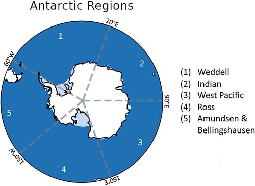
Assessment of skill is performed on both Pan-Antarctic and regional scales, using five regions defined in Bushuk et al. (2021) (Fig. 1). Each region is a sector spanning ${70}^{\circ }$ to ${80}^{\circ }$ longitude and containing different oceanographic and atmospheric conditions. For instance, sea ice area in the Ross sea is observed to vary substantially in the autumn, which M. M. Holland et al. (2017) attributed to springtime zonal winds driving high variability. Hosking et al. (2013) attributed changes in SIC in the Ross and Amundsen & Bellingshausen sectors to variability of the Amundsen Sea Low (ASL). Near-surface winds associated with a deepening of the ASL were observed to result in the intensification of winds near the Antarctic Peninsula as well as off the Ross ice shelf (P. R. Holland & Kwok, 2012). Evidently, such regionalization motivates investigation into what extent certain regions exhibit particularly high or low skill, potentially allowing for causes of such variability in skill due to local physical processes to be investigated. In addition to variations of predictive skill across these conventional zonal sectors, one might expect model skill to differ substantially near the ice edge relative to nearer the Antarctic continent. While outside the scope of this study, a more systematic investigation of SIE predictive skill would bring better insight into regional variations of predictability.

Fig. 1 Regions of the Antarctic defined in Bushuk et al. (2021), shown for a range of latitude ${45}^{\circ }$S to ${90}^{\circ }$S. The Weddell sector spans longitudes of ${60}^{\circ }$W to ${20}^{\circ }$E, the Indian sector spans ${20}^{\circ }$E to ${90}^{\circ }$E, the West Pacific sector from ${90}^{\circ }$E to ${160}^{\circ }$E, the Ross sector from ${160}^{\circ }$E to ${130}^{\circ }$W, and the Amundsen & Bellingshausen sector from ${130}^{\circ }$W to ${60}^{\circ }$W. Note the presence of ice shelves which are not dynamically modelled in CanCM4i and GEM-NEMO.

3 Seasonal forecasting skill of CanSIPSv2

In this section, we present an assessment of operational forecasting skill for CanSIPSv2 and its constituent models CanCM4i and GEM-NEMO in the Antarctic. We first consider skill of pan-Antarctic SIE, including analysis of the impacts of long-term trends in model prediction skill. Regional forecast skill is also considered. Next, prediction skill in models from the Geophysical Fluid Dynamics Laboratory is compared to that of CanSIPSv2. Finally, the influence of time period on predictive skill is considered.

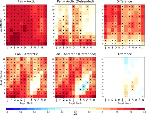
Prediction skill is presented as ACC plotted on a grid with axes target month and lead time (e.g. Fig. 2). For instance, the skill of a March lead-2 forecast would refer to the ACC for the target month of March, with the forecast initialized in January (two months prior to March). The skill of forecasts initialized for a particular initialization month can be read diagonally, such that a forecast initialized in January would consist of predictions for January lead-0, February lead-1, March lead-2, up to and including December lead-11. Predictive skill that is considered significant at a 95% level according to the procedure described in Section c is marked by a dot. If a forecast of significant skill also exceeds that of an anomaly persistence forecast, it is marked with a triangle. Filled triangles denote improvements over anomaly persistence that are statistically significant at the 95% confidence level (as determined from a bootstrap analysis). If the dynamical model forecast skill exceeds persistence but this difference is not statistically significant, the triangle is hollow. Crosses denote negative correlations that are significant at a 95% level.

Fig. 2 Anomaly correlation between the forecasted and observed pan-Arctic and Antarctic SIE for the years 1980–2010 as a function of lead time and target month, showing the relative effects of detrending. Rightmost column shows the difference between forecast skill and trend-independent forecast skill. Dots represent significance at the 95% level and triangles represent significance at the 95% level as well as skill exceeding an anomaly persistence forecast based on Had2CIS observational data. Filled triangles denote improvements over anomaly persistence that are statistically significant at the 95% confidence level (as determined from a bootstrap analysis). If the dynamical model forecast skill exceeds persistence but this difference is not statistically significant, the triangle is hollow. Note that target months in the Pan-Arctic skill plots are shifted by 6 months in order to align ice growth and melt seasons.

a Pan-Antarctic analysis

To contextualize the prediction skill of pan-Antarctic SIE, we first contrast this skill with pan-Arctic prediction skill as discussed in Martin et al. (2022). Prediction skill for CanSIPSv2 is illustrated in Fig. 2 for predictions of pan-Arctic SIE (upper row) and pan-Antarctic SIE (bottom row), where the horizontal axes (target month) for Arctic SIE predictions have been shifted by 6 months to align seasonal cycles.

In the absence of detrending, CanSIPSv2 shows significant skill in the Arctic across all target months and lead times, with the exception of May lead-4 and May lead-5. This skill frequently exceeds that of a persistence forecast throughout the year, excluding the melt season. In the southern hemisphere, forecasts are found to be skilful for target months ranging from January to August (mid austral summer to mid winter) with skill generally exceeding that of a persistence forecast. In contrast to model skill in the Arctic which remains generally significant throughout the year, the target months of September and December in the Antarctic show little skill for lead times of one month or greater (Fig. 2). Overall, forecast skill in the Arctic exceeds that of the Antarctic. This result is consistent with the presence of stronger trends in the Arctic, with previous results suggesting more model skill is to be derived from accurate predictions of such trends. The trends in the Antarctic are known to be much weaker (Parkinson, 2019), with the implication that less skill can be derived from accurate predictions of these weaker trends. This is also consistent with the greater reduction in Arctic forecast skill due to detrending compared to that in the Antarctic (rightmost column of Fig. 2). Interestingly, in spite of CanSIPSv2 showing decreased skill after detrending, such is not the case with CanCM4i. Instead, CanCM4i shows roughly equal skill before and after applying the detrending procedure – almost all skill loss in CanSIPSv2 due to detrending is on account of GEM-NEMO (Fig. A1 in the appendix.)

Detrending the SIE time series results in a substantial loss of forecast skill for CanSIPSv2 in the Arctic. This reduced skill is especially apparent for spring target months, where CanSIPSv2 shows little ability to predict SIE beyond lead times of 2 months. Significant forecast skill is observed for target months in boreal fall and winter, with the exception of November which shows significant low-to-moderate skill for lead times of 0 and 3 months. CanSIPSv2 also shows reduced skill with detrending in the Antarctic, though the reduction is not as substantial as is observed for the Arctic. Once again, this result is to be expected from the weaker trends in Antarctic sea ice relative to sea ice in the Arctic. No significant skill is shown in the target months of July to October beyond lead times of one month, suggesting that CanSIPSv2 is not adequately capturing the conditions associated with maximum SIE. The target months of January to April corresponding to a minimum in SIE also show significantly reduced skill with detrending for lead times greater than 4 months, though forecast skill in the target month of May remains significant across all lead times. Despite the smaller reduction of skill via detrending, CanSIPSv2 again shows lower forecast skill for sea ice in the Antarctic compared to the Arctic. However, this result is sensitive to the hindcast period considered. Fig. A2 (appendix) shows that when the hindcast period is extended to 2019 (instead of 2010), detrended skill in the Antarctic generally exceeds that of the Arctic. From this point onward, unless specified otherwise, we will present the forecast skill of detrended predictions for the hindcast period of 1980–2010.

b Regional variation in forecast skill

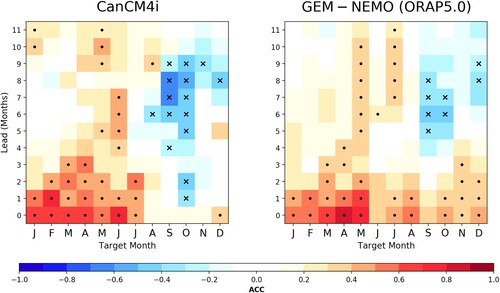
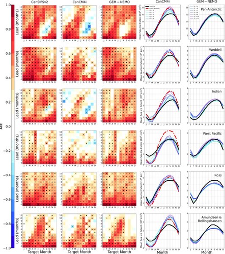
On a pan-Antarctic scale, of the two constituent models in CanSIPSv2, GEM-NEMO generally shows higher predictive skill, particularly for target months corresponding to maximum ice extent and the subsequent retreat (Fig. 3). These are also months in which CanCM4i shows substantial drifts toward the model's free-running climatology. Such pronounced drifts are not observed for GEM-NEMO. While such a systematic bias does not directly affect the ACC (which considers sea ice anomalies relative to mean SIE as per definition,) these initialization shocks can lead indirectly to reduced predictive skill (Mulholland et al., 2015).

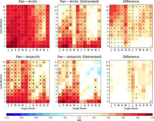
Fig. 3 Skill plots (for detrended predictions) and bias plots for each model and region. Each column corresponds to the model as labelled at the top, and each row corresponds to the region labelled in the right-most bias plot. Dots represent significance at the 95% level and triangles represent significance at the 95% level as well as skill exceeding an anomaly persistence forecast based on Had2CIS observational data. Filled triangles denote improvements over anomaly persistence that are statistically significant at the 95% confidence level (as determined from a bootstrap analysis). If the dynamical model forecast skill exceeds persistence but this difference is not statistically significant, the triangle is hollow. Crosses denote negative ACC that is significant at the 95% level. The coloured lines in the bias plots describe mean SIE, averaged over the years 1980–2010 for each calendar month as a function of the lead time (LT) indicated in the legend. The thicker black line describes Had2CIS observed SIE, also averaged over the years 1980–2010 for each calendar month. The dashed red line shows the mean SIE in a (freely running) historical CanCM4i run, averaged over said time period.

Substantial variation in forecast skill for different regions is also observed for CanCM4i and GEM-NEMO, (and by extension the combined system CanSIPSv2) as is illustrated in Fig. 3. The Weddell sector is the region of highest skill for CanSIPSv2. Outside of the October to December target months, CanSIPSv2 demonstrates significant skill for predictions made up to 8 months in advance, with skilful predictions produced up to a year in advance for the target months of January to July. Most of this long lead time skill appears to originate in GEM-NEMO. By contrast, CanCM4i shows little ability to consistently produce skilful forecasts beyond lead times of 5–7 months, depending on the season. For the October to December target months, CanCM4i shows relatively little predictive skill for lead times of 2 months or more. Similarly, GEM-NEMO shows no forecast skill for lead times of 4 months or more across these same target months. This fact suggests that both of the models are not adequately capturing sea ice retreat in this sector when initialized several months in advance. This is not unexpected, as a loss of predictability during ice retreat season in various regions of the Antarctic (such as the Weddell sector) has been well documented by previous studies (M. M. Holland et al., 2013; Libera et al., 2022; Marchi et al., 2018).

In contrast to the Weddell sector, the Indian sector is a region of generally lower skill for CanCM4i and GEM-NEMO. CanCM4i shows scarcely any skill beyond lead times of one month in target months January and February. Throughout other target months, little skill is found for lead times greater than three months. GEM-NEMO again shows generally higher skill than CanCM4i in this sector, with an ability to produce skilful predictions up to at least four months in advance across eight target months. As with the Weddell sector, both models show reduced skill at longer lead times during target months in the melt season, with CanCM4i and GEM-NEMO showing little skill beyond lead times of three or more for target months November and December. CanCM4i forecasts initialized in November show modest skill re-emergence, with vanishing skill for lead times of two to six months (i.e. January lead 2 to May lead 6 predictions) followed by an increase in skill for lead times up to and including 10 months. Similar, but weaker skill re-emergence is found for forecasts initialized in December, but forecasts initialized in October show no skill re-emergence. GEM-NEMO does not appear to demonstrate such skill re-emergence.

The West Pacific sector is also a region of generally low predictive skill. GEM-NEMO shows significant skill for target months in the melt season even at long lead times, particularly for target months November and December. GEM-NEMO demonstrates high skill for forecasts for the target month of May, yet almost no skill for forecasts for the subsequent target month of June (i,e., early austral winter.) GEM-NEMO also exhibits a diagonal skill feature indicative of a predictability barrier analogous to that observed for some regions in the Arctic (e.g. Martin et al., 2022): West Pacific SIE forecasts initialized in December are skilful out to much later lead times than for forecasts initialized in November, showing little skill for predictions made more than 1 month in advance. CanCM4i, however, does not show any features indicative of a predictability barrier in this sector, and shows decreased skill for target months throughout most of the year. It is also worth noting that CanCM4i exhibits an appreciable initialization shock for the months of January to April, wherein on average, the model drifts away from observations for increasing lead time and approaches the model's free-running climatology. As a possible consequence of the large initialization shock in CanCM4i, forecasts initialized in the months of January to April show significant skill at much longer lead times (outside of the target month of June) in GEM-NEMO than in CanCM4i.

In the Ross sector, CanCM4i and GEM-NEMO both show high skill for lead times up to seven months in target months ranging from September to December. The smallest prediction skill is observed in the target months of February to April, with predictions showing little skill beyond lead times of 4 months in GEM-NEMO. CanSIPSv2 forecasts are generally skilful up to lead times of 6–7 months for target months ranging from May to January, and up to lead times of 3–4 months otherwise. Interestingly, Marchi et al. (2018) find that ice-edge predictability in the Weddell and Ross sectors is greater than throughout the rest of the Southern Ocean. This result is consistent with CanSIPSv2 showing greater skill in these two sectors.

The Amundsen & Bellingshausen sector displays moderate predictive skill for the models considered. CanSIPSv2 demonstrates significant skill up to 10 months in advance for the target months of June, July, and August. For target months throughout the rest of the year, skill is generally significant up to two to five months in advance. CanSIPSv2 forecasts initialized for months in austral spring (specifically, August to October) show skill re-emergence, as skill is suddenly lost in the target month of February (leads 4–6) and then regained in the the target month of June (leads 8–10.) By contrast, forecasts initialized in December retain their skill up to eight months. CanCM4i and GEM-NEMO both show skill profiles that are similar to each other and to that of CanSIPSv2: Skill at longest lead times for target months during austral winter and decreased skill for other target months. GEM-NEMO generally shows skill at longer lead times (9–11 months) than CanCM4i (7–10 months) during winter target months, though CanCM4i shows skill at longer lead times for target months during austral spring and early austral summer than GEM-NEMO. GEM-NEMO also shows evidence of skill re-emergence, as is observed in the skill profile of CanSIPSv2.

c Possible causes of the skill difference between CanCM4i and GEM-NEMO

Fig. 3 indicates that GEM-NEMO is of generally higher predictive skill than CanCM4i on the pan-Antarctic scale. This difference is particularly noticeable for the target months of September to December, for lead times of up to three months. In order to investigate the differences between the two models, we consider the contribution of their respective SIT initializations to forecast skill, their drift from the observed climatological SIE for increasing lead times, as well as possible connections between ensemble spread and prediction skill.

The studies by Day et al. (2014), M. M. Holland et al. (2019), and Marchi et al. (2020) show that the initialization of SIT has a substantial influence on sea ice predictability in idealized model settings. Moreover, Blockley and Peterson (2018) show that real forecasts can be improved by using SIT observations in the assimilation system used to create the initial SIT conditions. Morioka et al. (2021) demonstrate similar improvements to real forecasts by initializing to a SIT analysis. CanCM4i initializes SIT through nudging toward a model climatology, with the disadvantage of this procedure being in its inability to capture short-term variability in sea ice and deviations from climatology. Initial SIT in GEM-NEMO is interpolated from the ORAP5 reanalysis, which provides reconstructed observations better suited to capturing short-term changes in SIC and SSTs, and hence should correspond to more realistic SIT conditions. To investigate the effectiveness of their SIT initialization, we consider the contribution of their respective sea ice volume (SIV) initializations to their hindcast skill, as well as their drift from the observed climatological SIE for increasing lead times. Note that SIV is inherently related to SIT, as it is defined as the pointwise product of sea ice area (SIA) and sea ice thickness (SIT).

We begin by investigating predictive skill of initial SIV conditions (derived from initial SIT data) as a statistical predictor of SIE. Such an analysis can provide insight into the effectiveness of their sea ice initialization. While it might be expected that the predictive skill of initial SIV is negligible in CanCM4i, in which initial sea ice conditions are obtained by relaxing towards a climatological mean, this is not the case. This is a consequence of the dependence of initial SIV on SIA, which is subject to interannual variability. It follows that this variability is reflected in the SIV conditions, possibly contributing to the skill of the model in predictions of SIE.

The skill of this statistical predictor is shown in Fig. 4 as a function of target month and lead time. Interestingly, despite their differences in initial SIV conditions, our statistical predictor shows somewhat similar skill in both models. However, Fig. 4 also shows that initial SIV in GEM-NEMO is a more skilful predictor of SIE for leads of 0 and 1 month in the target month of October, 0–3 months in the target month of November, and 0–2 months in the target month of December. By contrast, initial SIV in CanCM4i only shows significant skill as a predictor for the target month of December at lead 0. This feature likely corresponds with the greater predictive skill of GEM-NEMO at low leads during these same target months, compared to the relatively little skill of CanCM4i (Fig. 3, top row).

Fig. 4 Pan Antarctic sea ice extent forecast skill (detrended) of a statistical model that is based on the initial (Pan Antarctic mean) sea ice thickness. Dots represent significant positive ACC at the 95% level through bootstrapping, whereas crosses represent significant negative ACC at the 95% level.

If the initialized state of the model is sufficiently far from its ‘attractor’, forecast simulations can be dominated initially by adjustment to the attractor (model drift) with an associated loss of predictive skill. We investigate model drift through considering climatological means of hindcasts for different lead times and target months, as shown in the two rightmost columns of Fig. 3. The thick black line denotes Had2CIS climatological mean SIE for each month of the year. The coloured lines show climatological SIE for the respective model with a different line for each particular lead time. These plots suggest the presence of substantial inherent model biases in CanCM4i, manifesting as a strong drift away from its initialized states (close to the Had2CIS observations). This is particularly noticeable for the months around August to October, where the large seasonal amplitude results in a substantial overestimation of mean maximum sea ice cover. In contrast, GEM-NEMO shows relatively little drift from its initialized states. The model drift present in CanCM4i appears to correspond to the model approaching its freely running state (dashed red line in Fig. 3) for some regions, particularly for late austral winter and early austral spring months, when SIE is near its maximum. Furthermore, the drift rate of CanCM4i away from observations is especially high for early lead times. This large drift in CanCM4i from its initialized state may be an important factor in its relatively low predictive skill: The magnitude of the drift in a particular region and target month corresponds broadly with higher or lower skill. For instance, the Indian, West Pacific, and Amundsen & Bellingshausen sectors experience relatively large drift and display generally lower predictive skill compared to the Weddell and Ross sectors. We note that no freely-running simulation of GEM-NEMO is available, which precludes a systematic comparison of its climatology with observations. However, the smaller drift in GEM-NEMO from its initialized state suggests smaller inherent model biases than in CanCM4i. If these model biases in CanCM4i contribute at least partially to its skill, it is reasonable that the smaller biases in GEM-NEMO might result in better predictive skill overall compared to CanCM4i.

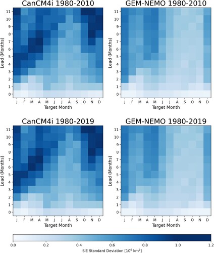
We additionally investigate the correspondence between ACC and ensemble spread by plotting the time-averaged standard deviations in ensemble predictions as a function of target month, and lead time (Fig. 5). As expected, ensemble standard deviations are lower in magnitude at short lead times (0–1 month) but generally increase in magnitude at longer lead times as the ensembles diverge from their initial states. CanCM4i ensemble predictions are subject to generally greater spread than GEM-NEMO at long lead times, especially for summer target months (November to January, leads 8 to 11 months). Moreover, CanCM4i ensemble predictions initialized in December appear to show less spread than those initialized a month prior. This ‘diagonal feature’ in Fig. 5 is also present in GEM-NEMO, though less pronounced. GEM-NEMO ensemble predictions for target months July to November show less spread than predictions for the remaining target months, regardless of lead time. There does not appear to be any significant dependence of ensemble spread on time period (discussed further in the next subsection), and there is no evident relationship between ensemble spread and predictive skill of the ensemble mean.

Fig. 5 Standard deviations of CanCM4i and GEM-NEMO ensemble predictions as a function of target month and lead time. Standard deviation is time-averaged over the period 1980–2010 (top row) and 1980–2019 (bottom row).

d Dependence on Time Period

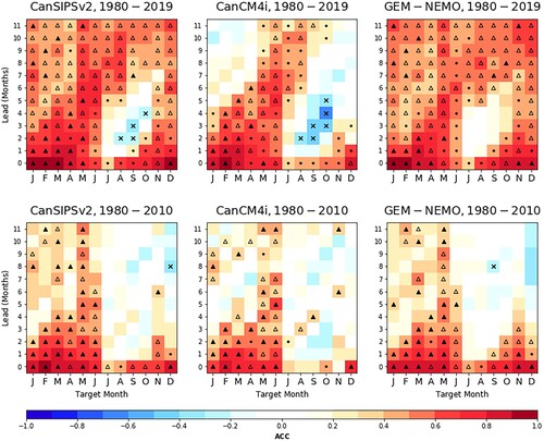
As described in Section b, the observational datasets used to initialize SIC in CanCM4i and GEM-NEMO were changed for hindcasts starting in 2013 and 2011, respectively. This change implies a potential dependence of skill on the time period considered. Furthermore, the hindcast period of 30 years is not particularly long and statistical measures of skill are expected to show some sampling variability. Predictive skills of CanCM4i, GEM-NEMO, and CanSIPSv2 for two time periods, 1980–2010 and 1980–2019, are shown in Fig. 6. Each model shows generally higher skill for the time period 1980–2019 relative to the shorter time period. This increase is especially apparent for the target months of July to December, and is larger for GEM-NEMO than for CanCM4i.

Fig. 6 Skill plots (detrended) for CanSIPSv2, CanCM4i, and GEM-NEMO, comparing Pan-Antarctic SIE prediction skill for two different time periods, 1980–2019 and 1980–2010. Markers are as in Fig. 3.

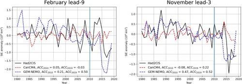
Fig. 7 shows two time series of observed and hindcast SIE anomalies, for February lead-9 and November lead-3. These target months and lead times show both higher skill for the full time period relative to forecast skill for 1980–2010 and a larger skill difference between CanCM4i and GEM-NEMO for the full time period. These time series indicate that the increase in skill for GEM-NEMO is due to the model capturing the large negative SIE anomalies occurring in recent years whereas CanCM4i does not accurately reproduce these large anomalies and hence does not see a substantial increase of forecast skill, resulting in the larger skill difference between models. The increase of skill in GEM-NEMO as a result of capturing these anomalies also substantially increases the skill of the forecast system, explaining the greater skill in CanSIPSv2 when using the time period 1980–2019 in contrast to 1980–2010. The ability of GEM-NEMO to represent this large event may result from the improved initialization in recent years, or may be a result of more accurate representations of the relevant physical processes in this model than in CanCM4i. We are unable to distinguish between these possibilities with the information available to us. Also note that there are no substantial differences in ensemble spread between the two time periods (Fig. 5), despite the substantial difference in predictive skill of the ensemble mean. This fact provides further evidence of a lack of connection for SIE between ensemble spread and predictive skill.

Fig. 7 SIE time series for Had2CIS observations (black), CanCM4i (red), and GEM-NEMO (blue). The left plot shows time series for February lead-9, and the right plot shows time series for November lead-3. A vertical blue line marks the year 2010. ${\mathrm{ACC}}_{2010}$ refers to the time period 1980–2010, and ${\mathrm{ACC}}_{2019}$ refers to the time period 1980–2019. Note that for GEM-NEMO ${\mathrm{ACC}}_{2019}>{\mathrm{ACC}}_{2010}$ the skill difference between CanCM4i and GEM-NEMO is generally greater for the full time period.

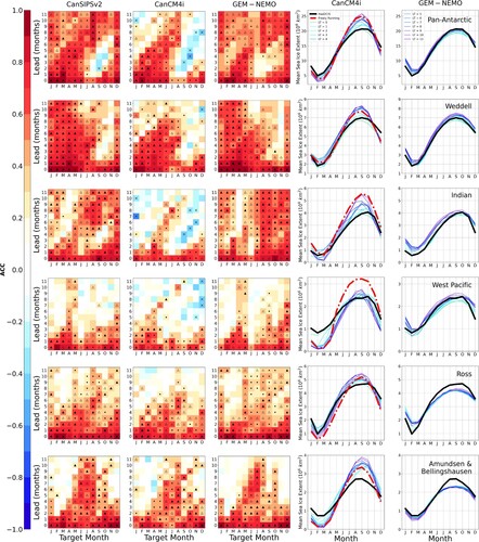
Predictive skill in some individual regions also shows dependence on time period (Fig. 8.) This dependence is most evident in the Weddell, Indian, and Ross sectors, though the West Pacific and Amundsen & Bellingshausen sectors do not show such a substantial dependence. In particular, GEM-NEMO shows substantially higher skill in the Weddell region for long leads in target months of August to December and enhanced skill for long leads across all target months in the Indian and Ross sectors for the longer 1980–2019 period compared to the 1980–2010 period. In contrast, CanCM4i does not show these increases in predictive skill for these three sectors.

Fig. 8 As Fig. 3, except based on hindcasts from 1980 to 2019.

e Comparison with GFDL Models

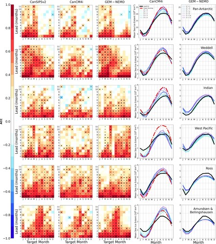
Bushuk et al. (2021) performed a similar assessment of seasonal prediction skill using a collection of forecast systems from the Geophysical Fluid Dynamics Laboratory (GFDL). This collection included the Forecast-oriented Low Ocean Resolution (FLOR) system as well as the Seamless System for Prediction and Earth System Research (SPEAR) with the latter available at two differing horizontal land-atmosphere resolutions of ${1.0}^{\circ }$ (SPEAR_LO) and ${0.5}^{\circ }$ (SPEAR_MED). As their study considers hindcasts over the time period of 1992–2018, our comparisons will be made with CanSIPSv2 forecast skill over the same period of time, which are shown in Fig. 9. Note the forecast skill over the 1992–2018 period is very similar to that over the 1980–2019 period (Fig. 8), except for the Ross Sea where skill over the 1992–2018 period is generally lower. It is also worth noting that the 1992–2018 time period considered in this study and that of Bushuk et al. (2021) approximately coincides with the period for which ocean satellite altimeter observations are available. The improved likeliness of accurate ocean initial conditions acts to indirectly constrain sea ice, and may result in improved skill in the GFDL systems for hindcasts initialized during this time interval. Initialization improvements become even greater with eventual implementation of Argo temperature and salinity profiles (Roemmich et al., 2004).

Fig. 9 As Fig. 3, except based on hindcasts from 1992 to 2018 to facilitate a comparison to Bushuk et al. (2021).

As with our findings, Bushuk et al. (2021) find that the forecast skill of the GFDL dynamical prediction systems generally exceeds that of an anomaly persistence forecast on a Pan-Antarctic scale. The SPEAR models show minimal skill in the target months of October, November, and December, corresponding to early-to-mid melt season in the southern hemisphere. By contrast, the FLOR model exhibits its maximum skill in the target month of December, followed by almost no significant skill in the subsequent target months of January, February, and March in which sea ice is near a minimum. For target months throughout the rest of the year (April to September), the SPEAR models show significant skill for lead times up to at least 7 months, whereas the FLOR model shows substantially lower skill (though generally still statistically significant). Similar to the SPEAR models, CanCM4i also shows little skill beyond lead times of 1 month in target months ranging from October to December. However, GEM-NEMO shows significant skill across most lead times in October and November, and across all lead times in the target month of December, perhaps suggesting that GEM-NEMO is better able to capture interannual variations in annual minimum SIE relative to SPEAR and CanCM4i. For target months throughout the rest of the year, CanCM4i is of generally lower skill than SPEAR, whereas GEM-NEMO is generally of equal or higher skill, with the exception of the target months of July to September at lead times of 1–5 months. Together, CanSIPSv2 shows generally greater skill than FLOR and SPEAR outside of the target months of July to September at lead times of 1–5 months.

The Weddell sector is a region of relatively high skill for both the SPEAR models and CanSIPSv2, with SPEAR_MED showing generally greater skill than SPEAR_LO. For predictions in the Indian sector, GEM-NEMO shows a similar skill pattern to the GFDL models, with generally significant skill exceeding persistence for most target months and lead times. In contrast, CanCM4i demonstrates low predictive skill in this region, with most of its skill concentrated in winter target months. SPEAR and FLOR show generally low skill in the West Pacific region as does CanSIPSv2. Bushuk et al. (2021) note the poor winter skill of SPEAR relative to the rest of the year, a feature that seems to be present in GEM-NEMO, and to a lesser extent CanCM4i. The forecast skill in the Ross Sea is substantially higher in CanSIPSv2 than in the GFDL models. Bushuk et al. (2021) suggest that the relatively low skill in this region may be a consequence of the high northward sea ice drift in the western Ross sea. If such is the case, then both CanCM4i and GEM-NEMO appear to effectively capture this drift. The GFDL models show the greatest skill in the target month of August up to 11 months lead time as is the case with CanCM4i. GEM-NEMO also shows significant skill for up to 11 months lead time, though the skill for the target month of August does not stand out relative to other target months. Predictive skill in the Amundsen & Bellingshausen sector is generally similar for both the GFDL models and CanSIPSv2: the models demonstrate significant skill for increasingly longer lead times until the target months of August and September, where the models are capable of accurately predicting SIE given lead times up to 10 or 11 months. This is followed by generally lower skill in subsequent target months ranging from October to December. SPEAR_LO and SPEAR_MED exhibit consistently significant skill for lead times up to 6 months. By contrast, GEM-NEMO shows significant skill only up to a lead time of 7 months in the target month of October and up to a lead time of 3 months in the target months of November and December. Target months throughout the rest of the year generally show similar results between SPEAR and GEM-NEMO.

We note that there may still be skill to be gained with respect to the GFDL seasonal prediction systems relative to that reported in Bushuk et al. (2021): Zhang et al. (2022) demonstrate that for sea ice prediction in the northern hemisphere on seasonal and sub-seasonal timescales, the skill of SPEAR shows notable improvement through assimilating SIC data (whose procedure is detailed by Zhang et al., 2021). It is possible that with this SIC data assimilation procedure, the GFDL systems may exhibit overall skill similar to or exceeding that of CanCM4i and GEM-NEMO for a number of initialization months.

4 Summary and conclusions

This study has evaluated the skill of the CanSIPSv2 dynamical forecasting system for seasonal forecasts of Antarctic sea ice. The skill of the two constituent models of CanSIPSv2 – CanCM4i and GEM-NEMO – were investigated in order to ascertain their individual contributions to overall forecast skill. This study considered both a Pan-Antarctic scale as well as individual regions of the Antarctic, so as to identify regions that contribute strongly to forecast skill. Finally, comparison was made with results from a previous detailed analysis of dynamical predictions of Antarctic SIE with GFDL models by Bushuk et al. (2021).

We found that accurate predictions of detrended pan-Antarctic SIE are only possible up to 1–3 months lead time for target months in austral winter and spring and up to 2–11 months lead time for target months in austral summer and fall, particularly for forecasts initialized in austral summer, based on 1980–2010 hindcasts. Target months and lead times that show significant skill generally exceed the skill of anomaly persistence forecasts, suggesting that model skill is not simply derived from persistence of sea ice. CanSIPSv2 showed no significant skill in its prediction of SIE for target months July to October at lead times of one month and greater. CanCM4i also showed similarly little significant skill for these target months and lead times. GEM-NEMO, however, showed significant forecast skill for lead times up to 2 months in the target months of October to December. CanCM4i and GEM-NEMO both also showed little significant skill for most of these target months and lead times. GEM-NEMO, however, showed significant forecast skill for lead times up to 2 months in the target months of October to December, suggesting that GEM-NEMO better captures summer sea ice conditions relative to CanCM4i, which may be related to a low SIE bias in CanCM4i, particularly in the Indian sector. Long-term trends in the Antarctic were observed to contribute to skill although not as much as has been found for Arctic sea ice predictions. Overall, based on 1980–2010 hindcasts, forecast skill in CanSIPSv2 was generally lower for predictions on a pan-Antarctic domain relative to a pan-Arctic domain, suggesting that forecasts of SIE on seasonal time scales in the Antarctic are less skilful than equivalent forecasts in the Arctic.

Predictive skill in GEM-NEMO generally exceeded that of CanCM4i. To investigate this difference in skill, we looked at the initialization of sea ice thickness (SIT) in both models as well as their temporal drift from initial states. The former investigation used sea ice volume (SIV, closely related to SIT) as a statistical predictor of SIE, whereby it was found that SIV acted as a better predictor of sea ice in GEM-NEMO for target months from August to December, for lead times of 0 to 3 months. This was consistent with the greater skill shown by GEM-NEMO on a Pan-Antarctic scale during these same target months and lead times. However, we also found a large drift from initial state (‘initialization shock’) in CanCM4i. GEM-NEMO also exhibited drift, though not to same extent as CanCM4i. Such drift appears to be especially prevalent in the Indian and West Pacific sectors, both of which are regions where the skill of GEM-NEMO generally exceeds the skill of CanCM4i. We hypothesize that the differences in skill between the two constituent models can largely be attributed to different SIT initializations for target months in the melt season, but also substantial drift in CanCM4i throughout various times of the calendar year.

The forecast skill of CanSIPSv2 showed a strong dependence on time period. When the hindcast period was extended to include the years 1980–2019, GEM-NEMO showed an appreciable increase in forecast skill. Over this time period, GEM-NEMO and CanSIPSv2 showed significant forecast skill for the majority of target months and lead times. CanCM4i also experienced an increase in forecast skill to a lesser extent showing significant skill at longer lead times in the target months of January to June and showing slightly increased skill for lead-0 forecasts in the target months of July to November. Two possible reasons for these increases in forecast skill were identified. First, both models (CanCM4i and GEM-NEMO) are subject to a change in initial SIC data sets in the years 2013 and 2011, respectively. Second, a comparison of predicted SIE time series with observed SIE time series showed that GEM-NEMO demonstrates an ability to capture the strong negative SIE anomalies present in recent years. Given the strength of these anomalies, accurate predictions of SIE over this recent time period resulted in a substantial increase in forecast skill. By contrast, CanCM4i showed little ability to capture these strong negative anomalies and hence did not experience such an increase in skill. The two potential causes of increased predictive skill are related, as the ability of GEM-NEMO to capture the large negative SIE anomaly may result from improved initialization. CanCM4i initializes SIT through nudging to a climatology. The disadvantage of such a procedure is in its inability to capture short-term variability in sea ice and deviations from climatology. By contrast, initial SIT in GEM-NEMO is interpolated from the ORAP5 reanalysis until 2010, which provides reconstructed observations better suited to capturing short-term changes in SIC and SSTs, and hence should correspond to more realistic SIT conditions.

We contrasted our results with those of Bushuk et al. (2021), who performed a similar analysis with the FLOR and SPEAR models from GFDL. Overall, the skill of CanSIPSv2 was found to generally exceed that of FLOR and SPEAR outside of target months ranging from July to September, for lead times from 1–5 months.

Given the limited amount of attention Antarctic sea ice has received in regard to dynamical forecasts, more studies of sea ice predictability with different models would be largely beneficial for comparing regional predictability. As noted by Massonnet et al. (2023), group forecasts that combine the predictions of many such models can serve to average out errors specific to any individual model. Further subdividing the regions may also have merit – particularly in identifying small regions of inherently lower or higher predictability, or with respect to latitude as well as longitude. For instance, Kacimi and Kwok (2020) divide the Weddell sector into a western and eastern part, the former being home to the cyclonic Weddell gyre, a substantial influence on sea ice dynamics in the region. This same study is also important in that it provides an opportunity for the development of SIT data products from CryoSat-2 and IceSat-2 satellite freeboard, snow depth, and ice thickness retrievals. Given the known importance of proper SIT initialization for skilful forecasts in the Arctic (e.g. Bonan et al., 2019; Bushuk et al., 2020; M. M. Holland et al., 2019), such a product could greatly improve the prediction skill of dynamical sea ice models. Another approach to improving SIT initialization is through statistical models such as that developed for the Arctic by Dirkson et al. (2017). Unfortunately, their model cannot be directly applied to SIT in the Antarctic. However, the study and development of a similar statistical model in the context of the Southern Ocean could greatly improve the accuracy of initial SIT conditions, leading to improvements in forecasts of SIE. There also is merit in investigating the relationship between initial ocean water mass and sea ice forecast skill: Uotila et al. (2019) remark that the ORAP5 reanalysis shows relatively low water transport through the Drake Passage (in the Amundsen & Bellingshausen sector) relative to an assessment by Donohue et al. (2016). Given that GEM-NEMO SIT and ocean conditions are initialized from ORAP5 until 2010, this may manifest itself as low skill for the target month of December for the time period 1980–2010 (Fig. 6). By contrast, GEM-NEMO shows substantial improvement in the target month of December for the longer time periods which include the years for which the model is initialized via CCMEP GIOPS. It may be worth investigating the extent to which this improvement is due to improvements in capturing water transport through the Drake Passage.

Disclosure statement

The authors declare that the research was conducted in the absence of any potential conflicts of interest.

Additional information

Funding

This research was made possible by the funding provided by Environment and Climate Change Canada (ECCC). Adam Monahan acknowledges the support of the Natural Sciences and Engineering Research Council of Canada (NSERC) (funding reference RGPIN-2019-204986).

Appendix

Fig. A1 CanCM4i and GEM-NEMO anomaly correlations between forecasted and observed pan-Antarctic SIE for the years 1980-2010 as a function of lead time and target month, showing the relative effects of detrending on each model. Rightmost column shows the difference between forecast skill and trend-independent forecast skill. Significance markers (dots, triangles, and crosses) are as defined in Fig. 2.

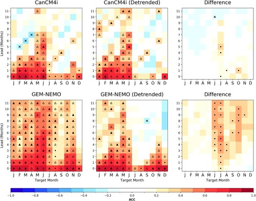
Fig. A2 As Fig. 2, except based on the hindcasts from 1980 to 2019.

References

- Behringer, D. W., Ji, M., & Leetmaa, A. (1998). An improved coupled model for ENSO prediction and implications for ocean initialization. Part I: The ocean data assimilation system. Monthly Weather Review, 126(4), 1013–1021. https://doi.org/10.1175/1520-0493(1998)126<1013:AICMFE>2.0.CO;2
- Blockley, E. W., & Peterson, K. A. (2018). Improving Met Office seasonal predictions of Arctic sea ice using assimilation of CryoSat-2 thickness. The Cryosphere, 12(11), 3419–3438. https://doi.org/10.5194/tc-12-3419-2018
- Bonan, D. B., Bushuk, M., & Winton, M. (2019). A spring barrier for regional predictions of summer Arctic sea ice. Geophysical Research Letters, 46(11), 5937–5947. https://doi.org/10.1029/2019GL082947
- Buehner, M., McTaggart-Cowan, R., Beaulne, A., Charette, C., Garand, L., Heilliette, S., Lapalme, E., Laroche, S., Macpherson, S. R., Morneau, J., & Zadra, A. (2015). Implementation of deterministic weather forecasting systems based on ensemble-variational data assimilation at environment Canada. Part I: The global system. Monthly Weather Review, 143(7), 2532–2559. https://doi.org/10.1175/MWR-D-14-00354.1
- Bushuk, M., Msadek, R., Winton, M., Vecchi, G., Yang, X., Rosati, A., & Gudgel, R. (2018). Regional Arctic sea–ice prediction: Potential versus operational seasonal forecast skill. Climate Dynamics, 52(5–6), 2721–2743. https://doi.org/10.1007/s00382-018-4288-y
- Bushuk, M., Winton, M., Bonan, D. B., Blanchard-Wrigglesworth, E., & Delworth, T. L. (2020). A mechanism for the Arctic sea ice spring predictability Barrier. Geophysical Research Letters, 47(13). https://doi.org/10.1029/2020GL088335
- Bushuk, M., Winton, M., Haumann, F. A., Delworth, T., Lu, F., Zhang, Y., Jia, L., Zhang, L., Cooke, W., Harrison, M., Hurlin, B., Johnson, N. C., Kapnick, S. B., McHugh, C., Murakami, H., Rosati, A., Tseng, K.-C., A. T. Wittenberg, Yang, X., & Zeng, F. (2021). Seasonal prediction and predictability of regional Antarctic sea ice. Journal of Climate, 34(15), 6207–6233. https://doi.org/10.1175/JCLI-D-20-0965.1
- Cavanagh, R. D., Melbourne-Thomas, J., Grant, S. M., Barnes, D. K. A., Hughes, K. A., Halfter, S., Meredith, M. P., Murphy, E. J., Trebilco, R., & Hill, S. (2021). Future risk for Southern Ocean ecosystem services under climate change. Frontiers in Marine Science, 7. https://doi.org/10.3389/fmars.2020.615214
- Chen, D., & Yuan, X. (2004). A Markov model for seasonal forecast of Antarctic sea ice. Journal of Climate, 17(16), 3156–3168. https://doi.org/10.1175/1520-0442(2004)017<3156:AMMFSF>2.0.CO;2
- Day, J. J., Hawkins, E., & Tietsche, S. (2014). Will Arctic sea ice thickness initialization improve seasonal forecast skill? Geophysical Research Letters, 41(21), 7566–7575. https://doi.org/10.1002/2014GL061694
- Dirkson, A., Denis, B., Sigmond, M., & Merryfield, W. J. (2021). Development and calibration of seasonal probabilistic forecasts of ice-free dates and freeze-up dates. Weather and Forecasting, 36(1), 301–324. https://doi.org/10.1175/WAF-D-20-0066.1
- Dirkson, A., Merryfield, W. J., & Monahan, A. (2017). Impacts of sea ice thickness initialization on seasonal Arctic sea ice predictions. Journal of Climate, 30(3), 1001–1017. https://doi.org/10.1175/JCLI-D-16-0437.1
- Donohue, K. A., Tracey, K. L., Watts, D. R., Chidichimo, M. P., & Chereskin, T. K. (2016). Mean Antarctic circumpolar current transport measured in Drake Passage. Geophysical Research Letters, 43(22), 11760–11767. https://doi.org/10.1002/2016GL070319
- Flato, G. M., & Hibler, W. (1992). Modeling pack ice as a cavitating fluid. Journal of Physical Oceanography, 22(6), 626–651. https://doi.org/10.1175/1520-0485(1992)022<0626:MPIAAC>2.0.CO;2
- Graham, R. M., Itkin, P., Meyer, A., Sundfjord, A., Spreen, G., Smedsrud, L. H., G. E. Liston, Cheng, B., Cohen, L., Divine, D., Fer, I., Fransson, A., Gerland, S., Haapala, J., Hudson, S. R., Johansson, A. M., King, J., Merkouriadi, I., Peterson, A. K., …Granskog, M. A. (2019). Winter storms accelerate the demise of sea ice in the Atlantic sector of the Arctic Ocean. Scientific Reports, 9(1), 9222. https://doi.org/10.1038/s41598-019-45574-5
- Grant, S. M., Hill, S. L., Trathan, P. N., & Murphy, E. J. (2013). Ecosystem services of the Southern Ocean: Trade-offs in decision-making. Antarctic Science, 25(5), 603–617. https://doi.org/10.1017/S0954102013000308
- Holland, M. M., Blanchard-Wrigglesworth, E., Kay, J., & Vavrus, S. (2013). Initial-value predictability of Antarctic sea ice in the Community Climate System Model 3. Geophysical Research Letters, 40(10), 2121–2124. https://doi.org/10.1002/grl.50410
- Holland, M. M., Landrum, L., Bailey, D., & Vavrus, S. (2019). Changing seasonal predictability of Arctic summer sea ice area in a warming climate. Journal of Climate, 32(16), 4963–4979. https://doi.org/10.1175/JCLI-D-19-0034.1
- Holland, M. M., Landrum, L., Raphael, M., & Stammerjohn, S. (2017). Springtime winds drive Ross Sea ice variability and change in the following autumn. Nature Communications, 8(1), 731–738. https://doi.org/10.1038/s41467-017-00820-0
- Holland, P. R., & Kwok, R. (2012). Wind-driven trends in Antarctic sea-ice drift. Nature Geoscience, 5(12), 872–875. https://doi.org/10.1038/ngeo1627
- Hosking, J. S., Orr, A., Marshall, G. J., Turner, J., & Phillips, T. (2013). The influence of the Amundsen-Bellingshausen Seas low on the climate of West Antarctica and its representation in coupled climate model simulations. Journal of Climate, 26(17), 6633–6648. https://doi.org/10.1175/JCLI-D-12-00813.1
- Hunke, E., & Lipscomb, W. (2010). CICE: The Los Alamos sea ice model documentation and software user's manual version 4.1 LA-CC-06-012 (Technical Report). LA-CC-06-012.
- Kacimi, S., & Kwok, R. (2020). The Antarctic sea ice cover from ICESat-2 and CryoSat-2: Freeboard, snow depth, and ice thickness. The Cryosphere, 14(12), 4453–4474. https://doi.org/10.5194/tc-14-4453-2020
- Kohout, A. L., Williams, M. J. M., Dean, S. M., & Meylan, M. H. (2014). Storm-induced sea-ice breakup and the implications for ice extent. Nature (London), 509(7502), 604–607. https://doi.org/10.1038/nature13262
- Libera, S., Hobbs, W., Klocker, A., Meyer, A., & Matear, R. (2022). Ocean-sea ice processes and their role in multi-month predictability of Antarctic sea ice. Geophysical Research Letters, 49(8), e2021GL097047. https://doi.org/10.1029/2021GL097047
- Lin, H., Gagnon, N., Beauregard, S., Muncaster, R., Markovic, M., Denis, B., & Charron, M. (2016). GEPS-based monthly prediction at the Canadian Meteorological Centre. Monthly Weather Review, 144(12), 4867–4883. https://doi.org/10.1175/MWR-D-16-0138.1
- Lin, H., Merryfield, W. J., Muncaster, R., Smith, G. C., Markovic, M., Dupont, F., Roy, F., Lemieux, J.-F., Dirkson, A., Kharin, V. V., Lee, W.-S., Charron, M., & Erfani, A. (2020). The Canadian seasonal to interannual prediction system version 2 (CanSIPSv2). Weather and Forecasting, 35(4), 1317–1343. https://doi.org/10.1175/WAF-D-19-0259.1
- Maksym, T. (2019). Arctic and Antarctic sea ice change: Contrasts, commonalities, and causes. Annual Review of Marine Science, 11(1), 187–213. https://doi.org/10.1146/annurev-marine-010816-060610
- Marchi, S., Fichefet, T., & Goosse, H. (2020). Respective influences of perturbed atmospheric and ocean-sea ice initial conditions on the skill of seasonal Antarctic sea ice predictions: A study with NEMO3.6-LIM3. Ocean Modelling (Oxford), 148, 101591. https://doi.org/10.1016/j.ocemod.2020.101591
- Marchi, S., Fichefet, T., Goosse, H., Zunz, V., Tietsche, S., Day, J. J., & Hawkins, E. (2018). Reemergence of Antarctic sea ice predictability and its link to deep ocean mixing in global climate models. Climate Dynamics, 52(5-6), 2775–2797. https://doi.org/10.1007/s00382-018-4292-2
- Martin, J. Z., Sigmond, M., & Monahan, A. (2022). Improved seasonal forecast skill of Arctic sea ice in CanSIPS version 2. Weather and Forecasting.
- Martinson, D. G. (2012). Antarctic circumpolar current's role in the Antarctic ice system: An overview. Palaeogeography, Palaeoclimatology, Palaeoecology, 335-336, 71–74. https://doi.org/10.1016/j.palaeo.2011.04.007
- Massonnet, F., Barreira, S., Barthélemy, A., Bilbao, R., Blanchard-Wrigglesworth, E., Blockley, E., Bromwich, D. H., Bushuk, M., Dong, X., Goessling, H. F., Hobbs, W., Iovino, D., Lee, W.-S., Li, C., Meier, W. N., Merryfield, W. J., Moreno-Chamarro, E., Morioka, Y., Li, X., …Yuan, X. (2023). SIPN South: Six years of coordinated seasonal Antarctic sea ice predictions. Frontiers in Marine Science, 10. https://doi.org/10.3389/fmars.2023.1148899
- Massonnet, F., Reid, P., Lieser, J. L., Bitz, C. M., Fyfe, J., & Hobbs, W. (2018). Assessment of February 2018 sea-ice forecasts for the Southern Ocean (Technical Report). University of Tasmania. https://doi.org/10.4226/77/5b343caab0498
- Massonnet, F., Reid, P., Lieser, J. L., Bitz, C. M., Fyfe, J., & Hobbs, W. (2019). Assessment of summer 2018–2019 sea-ice forecasts for the Southern Ocean (Technical Report). University of Tasmania. https://doi.org/10.25959/100.00029984
- Meredith, M., Sommerkorn, M., Cassotta, S., Derksen, C., Ekaykin, A., Hollowed, A.Kofinas, G., Mackintosh, A., Melbourne-Thomas, J., Muelbert, M. M. C., Ottersen, G., Pritchard, H., & Schuur, E. A. G. (2019). Polar regions. Chapter 3, IPCC special report on the ocean and cryosphere in a changing climate. https://doi.org/10.1017/9781009157964.005
- Merryfield, W. J., Lee, W. S., Boer, G. J., Kharin, V. V., Scinocca, J. F., Flato, G. M., Ajayamohan, R. S., Fyfe, J. C., Tang, Y., & Polavarapu, S. (2013). The Canadian seasonal to interannual prediction system. Part I: Models and initialization. Monthly Weather Review, 141(8), 2910–2945. https://doi.org/10.1175/MWR-D-12-00216.1
- Morioka, Y., Iovino, D., Cipollone, A., Masina, S., & Behera, S. K. (2021). Summertime sea-ice prediction in the Weddell Sea improved by sea-ice thickness initialization. Scientific Reports, 11(1), 11475–11475. https://doi.org/10.1038/s41598-021-91042-4
- Mulholland, D. P., Laloyaux, P., Haines, K., & M. A. Balmaseda (2015). Origin and impact of initialization shocks in coupled atmosphere-ocean forecasts. Monthly Weather Review, 143(11), 4631–4644. https://doi.org/10.1175/MWR-D-15-0076.1
- Parkinson, C. L. (2019). A 40-y record reveals gradual Antarctic sea ice increases followed by decreases at rates far exceeding the rates seen in the Arctic. Proceedings of the National Academy of Sciences – PNAS, 116(29), 14414–14423. https://doi.org/10.1073/pnas.1906556116
- Pehlke, H., Brey, T., Konijnenberg, R., & Teschke, K. (2022). A tool to evaluate accessibility due to sea-ice cover: A case study of the Weddell Sea, Antarctica. Antarctic Science, 34(1), 97–104. https://doi.org/10.1017/S0954102021000523
- Perovich, D. K., & Polashenski, C. (2012). Albedo evolution of seasonal Arctic sea ice. Geophysical Research Letters, 39(8). https://doi.org/10.1029/2012GL051432
- Pertierra, L., Santos-Martin, F., Hughes, K. A., Avila, C., Caceres, J. O., De Filippo, D., Gonzalez, S., Grant, S. M., Lynch, H., Marina-Montes, C., Quesada, A., Tejedo, P., Tin, T., & Benayas, J. (2021). Ecosystem services in Antarctica: Global assessment of the current state, future challenges and managing opportunities. Ecosystem Services, 49, 101299. https://doi.org/10.1016/j.ecoser.2021.101299
- Reiss, C. S., Cossio, A., Santora, J. A., Dietrich, K. S., Murray, A., Mitchell, B. G., Walsh, J., Weiss, E. L., Gimpel, C., Jones, C. D., & Watters, G. M. (2017). Overwinter habitat selection by Antarctic krill under varying sea-ice conditions: Implications for top predators and fishery management. Marine Ecology. Progress Series (Halstenbek), 568, 1–16. https://doi.org/10.3354/meps12099
- Reynolds, R. W., Rayner, N. A., Smith, T. M., Stokes, D. C., & Wang, W. (2002). An improved in situ and satellite SST analysis for climate. Journal of Climate, 15(13), 1609–1625. https://doi.org/10.1175/1520-0442(2002)015<1609:AIISAS>2.0.CO;2
- Roemmich, D., Riser, S., Davis, R., & Desaubies, Y. (2004). Autonomous profiling floats: Workhorse for broad-scale ocean observations. Marine Technology Society Journal, 38(2), 21–29. https://doi.org/10.4031/002533204787522802
- Sigmond, M., Fyfe, J. C., Flato, G. M., Kharin, V. V., & Merryfield, W. J. (2013). Seasonal forecast skill of Arctic sea ice area in a dynamical forecast system. Geophysical Research Letters, 40(3), 529–534. https://doi.org/10.1002/grl.50129
- Smith, G. C., Roy, F., Reszka, M., Surcel Colan, D., He, Z., Deacu, D., Belanger, J.-M., Skachko, S., Liu, Y., Dupont, F., Lemieux, J.-F., Beaudoin, C., Tranchant, B., Drévillon, M., Garric, G., Testut, C.-E., Lellouche, J.-M., Pellerin, P., Ritchie, H., …Lajoie, M. (2016). Sea ice forecast verification in the Canadian global ice ocean prediction system. Quarterly Journal of the Royal Meteorological Society, 142(695), 659–671. https://doi.org/10.1002/qj.2555
- Smith, T. M., & Reynolds, R. W. (2004). Improved extended reconstruction of SST (1854–1997). Journal of Climate, 17(12), 2466–2477. https://doi.org/10.1175/1520-0442(2004)017<2466:IEROS>2.0.CO;2
- Smith Jr, W. O., & Comiso, J. C. (2008). Influence of sea ice on primary production in the Southern Ocean: A satellite perspective. Journal of Geophysical Research, 113(C5), C05S93-n/a. https://doi.org/10.1029/2007JC004251
- Steele, M., & Boyd, T. (1998). Retreat of the cold halocline layer in the Arctic Ocean. Journal of Geophysical Research: Oceans, 103(C5), 10419–10435. https://doi.org/10.1029/98JC00580
- Steele, M., Morley, R., & Ermold, W. (2001). PHC: A global ocean hydrography with a high-quality Arctic Ocean. Journal of Climate, 14(9), 2079–2087. https://doi.org/10.1175/1520-0442(2001)014<2079:PAGOHW>2.0.CO;2
- Steiner, N. S., Bowman, J., Campbell, K., Chierici, M., Eronen-Rasimus, E., Falardeau, M., Flores, H., Fransson, A., Herr, H., Insley, S. J., Kauko, H. M., Lannuzel, D., Loseto, L., Lynnes, A., Majewski, A., Meiners, K. M., Miller, L. A., L. N. Michel, Moreau, S., …Wongpan, P. (2021, October). Climate change impacts on sea-ice ecosystems and associated ecosystem services. Elementa: Science of the Anthropocene, 9(1), 00007. https://doi.org/10.1525/elementa.2021.00007
- Titchner, H. A., & Rayner, N. A. (2014). The Met Office Hadley Centre sea ice and sea surface temperature data set, version 2: 1. Sea ice concentrations. Journal of Geophysical Research: Atmospheres, 119(6), 2864–2889. https://doi.org/10.1002/2013JD020316
- Tivy, A., Howell, S. E. L., Alt, B., McCourt, S., Chagnon, R., Crocker, G., Carrieres, T., & Yackel, J. J. (2011). Trends and variability in summer sea ice cover in the Canadian Arctic based on the Canadian Ice Service Digital Archive, 1960–2008 and 1968–2008. Journal of Geophysical Research, 116(C3). https://doi.org/10.1029/2009JC005855
- Uotila, P., Goosse, H., Haines, K., Chevallier, M., Barthélemy, A., Bricaud, C., Carton, J., Fuckar, N., Garric, G., Iovino, D., Kauker, F., Korhonen, M., Lien, V. S., Marnela, M., Massonnet, F., Mignac, D., Peterson, K. A., Sadikni, R., Shi, L., …Zhang, Z. (2019). An assessment of ten ocean reanalyses in the polar regions. Climate Dynamics, 52(3-4), 1613–1650. https://doi.org/10.1007/s00382-018-4242-z
- Uotila, P., Vihma, T., Pezza, A. B., Simmonds, I., Keay, K., & Lynch, A. H. (2011). Relationships between Antarctic cyclones and surface conditions as derived from high-resolution numerical weather prediction data. Journal of Geophysical Research, 116(D7). https://doi.org/10.1029/2010JD015358
- Valkonen, E., Cassano, J., & Cassano, E. (2021). Arctic cyclones and their interactions with the declining sea ice: A recent climatology. Journal of Geophysical Research: Atmospheres, 126(12). https://doi.org/10.1029/2020JD034366
- Zampieri, L., Goessling, H. F., & Jung, T. (2019). Predictability of Antarctic sea ice edge on subseasonal time scales. Geophysical Research Letters, 46(16), 9719–9727. https://doi.org/10.1029/2019GL084096
- Zhang, Y. F., Bushuk, M., Winton, M., Hurlin, B., Delworth, T., Harrison, M., Jia, L., Lu, F., Rosati, A., & Yang, X. (2022). Subseasonal-to-seasonal Arctic sea ice forecast skill improvement from sea ice concentration assimilation. Journal of Climate, 35(13), 4233–4252. https://doi.org/10.1175/JCLI-D-21-0548.1
- Zhang, Y. F., Bushuk, M., Winton, M., Hurlin, B., Yang, X., Delworth, T., & Jia, L. (2021). Assimilation of satellite-retrieved sea ice concentration and prospects for September predictions of Arctic sea ice. Journal of Climate, 34(6), 2107–2126. https://doi.org/10.1175/JCLI-D-20-0469.1
- Zuo, H., Balmaseda, M. A., & Mogensen, K. (2017). The new eddy-permitting ORAP5 ocean reanalysis: Description, evaluation and uncertainties in climate signals. Climate Dynamics, 49(3), 791–811. https://doi.org/10.1007/s00382-015-2675-1