Metabarcoding for plant pathologists

Abstract

Metabarcoding is a method that uses high-throughput sequencing to characterize microbial communities. This approach involves PCR-based amplification of a single locus from environmental DNA of communities of organisms, sequencing the resulting amplicons, and comparing those sequences to reference databases to infer the taxonomic identities of organisms present. By comparing the identity and number of associated sequences between samples, the data produced by metabarcoding can be used to reveal differences among sample types and identify biological variables that correlate with differences. However, metabarcoding is affected by a myriad of technical factors including sampling technique, DNA extraction methods, as well as choice of primers, locus for PCR amplification, and data analysis procedures. The resulting outputs will be both complex and semi-quantitative. The methods used can affect reliability of results including false positives and negatives, especially if the goal is to confidently survey the presence of plant pathogens. This article reviews the status of metabarcoding as it pertains to plant pathology and provides guidance on experimental design and analyses of bacterial, fungal, and oomycete datasets.

Résumé

Le métacodage à barres est une méthode qui utilize le séquençage à haut débit pour caractériser les communautés microbiennes. Cette approche est basée sur l’amplification par PCR d’un locus unique issu de l’ADN environnemental de communautés d’organismes, sur le séquençage des amplicons qui en résultent et la comparaison de ces séquences avec des banques de données pour inférer les identités taxinomiques des organismes présents. En comparant le degré d’identité et le nombre de séquences associées entre les échantillons, les données produites par le métacodage à barres peuvent être utilisées pour souligner des différences entre les types d’échantillons et définir les variables biologiques qui corrélèrent ces différences. Toutefois, le métacodage à barres est influencé par une myriade de facteurs techniques, y compris la méthode d’échantillonnage, celles d’extraction de l’ADN ainsi que le choix des amorces, le locus choisi pour l’amplification par PCR et les procédures d’analyse des données. Les extrants qui en résultent seront à la fois complexes et semi-quantitatifs. Les méthodes utilisées peuvent influencer la fiabilité des résultats, y compris de faux positifs et de faux négatifs, en particulier si le but est d’étudier en toute confiance la présence d’agents phytopathogènes. Cet article examine la pertinence du métacodage à barres à l’égard de la phytopathologie et fournit des indications quant à la conception expérimentale et aux analyses des jeux de données relatifs aux bactéries, aux champignons et aux oomycètes.

Keywords:

• best practices
• community
• high-throughput sequencing
• metabarcoding
• microbiome
• plant pathology

Mots clés:

• Meilleures pratiques
• communauté
• séquençage à haut débit
• métacodage à barres
• microbiome
• phytopathologie

Introduction

Pathogens and other pests continue to emerge at accelerated rates in agricultural, forest and natural ecosystems (Fisher et al. 2012). This trend is likely driven by the combined effects of climate change, increased human travel, and trade worldwide. To effectively diagnose and mitigate pathogen emergence, plant pathologists must develop a new generation of tools that can lead to rapid and effective responses. Often, molecular techniques such as PCR and Sanger sequencing allow detection and characterization of plant pathogens with greater taxonomic resolution and speed than morphological characterization (Sanzani et al. 2014). However, detection using molecular techniques typically applies only to well-characterized pathogens because of reliance on isolation, baiting and/or culturing methods. Field-based detection strategies such as lateral flow devices and their associated assays have also been developed for rapid detection of plant pathogens (De Boer and López 2012), but these approaches rely on the use of specific probes and primers and can only be used to target known and specific pathogens. In contrast, newer high-throughput metabarcoding and metagenomics methods detect and survey species and emerging plant pathogens directly from environmental samples (Piombo et al. 2021).

Metabarcoding is a high-throughput sequencing approach that identifies multiple taxonomic lineages from DNA extracted directly from plants, soil, water, and other sample types (Taberlet et al. 2012). Unlike conventional molecular diagnostics in which a region unique to a specific pathogen is used for identification, metabarcoding uses a region (i.e. ‘barcode’) that can identify groups within taxa, often to the genus and sometimes to the species level. Primers are designed that anneal to conserved regions flanking a highly variable barcode, such as portions of the 16S rRNA gene for bacteria (Janda and Abbott 2007), the ITS region for fungi or oomycetes (White et al. 1990; Sapkota and Nicolaisen 2015; Riit et al. 2016), or the mitochondrial rps10 gene for oomycetes (Foster et al. 2022). Amplified fragments are sequenced using a high-throughput platform, such as Illumina (http://www.illumina.com), and the resulting sequences are aligned and compared to a database of curated sequences to infer taxonomic identities of community members, thus uncovering known and unknown taxa or variants relative to reference databases.

A related method known as ‘shotgun’ metagenomics involves sequencing the DNA of all organisms within a sample and assembling the reads together into partial or full genome sequences, which can then be annotated. Predictions of genes and their functions can subsequently be made (Piombo et al. 2021). In shotgun metagenomics, unlike metabarcoding, a random subset of all DNA in the sample is sequenced regardless of locus or organism. While a metagenomics approach is especially suited to groups of organisms for which no common marker genes are shared, such as viruses (Edwards and Rohwer 2005), this method comes at the expense of lower sample throughput relative to metabarcoding (Quince et al. 2017). Though both approaches provide plant pathologists a snapshot of the communities of organisms present within sampled environments, in this review we will focus on metabarcoding as it is currently the most dominant method used by plant pathologists who are examining bacterial, fungal, and oomycete communities.

Metabarcoding has the potential to be a powerful tool for plant pathology research. Possible applications include identifying phytopathogens (Sapp et al. 2016), determining the effect of a treatment on the diversity of pathogens (Sylla et al. 2013), or testing specificity and efficacy of new biocontrol agents (Sow et al. 2019). This review provides a basic introduction on how to conduct, analyze, and interpret data from metabarcoding experiments. Topics addressed include sampling strategies, considerations related to DNA extraction and PCR amplification, the selection of barcodes, primers, and controls, as well as methods for data analysis.

Sampling strategies

Careful consideration of sampling strategy is necessary for making accurate inferences on community structure. Given the complexities of sampling, it is advisable to test procedures on a small number of samples before embarking on a full-scale experiment. Before collection, several decisions must be made to ensure that samples are representative of the target community (Dickie et al. 2018). This can be quite difficult because biomass of a sample is often small and microbial composition can be spatially and temporally variable (Beckers et al. 2017; Sapkota et al. 2017). To account for the latter, standardizing the age/condition of plants or tissues sampled is important because communities present are affected by host factors such as age, lifecycle stage, genotype, and health (Wagner et al. 2016). The sampling technique used can influence the community composition. It is likely that commonly used sampling techniques and intensities are insufficient to capture all the natural variability of plant microbial communities (Bullington et al. 2021). Therefore, sampling strategies should be designed to capture as much variation relevant to the experimental question as possible.

Sampling from water, soil, plant roots, and other plant tissues each pose their own challenges for collecting in a consistent and representative way. Soil and root samples are heterogenous. For example, different layers of the soil have differences in properties such as nitrogen availability, organic matter concentration, salinity, temperature, pH, and texture, which give rise to spatial variations in the diversity and abundance of microbial taxa (Fierer 2017; Bastida et al. 2021). When collecting soil samples, there should be a defined protocol describing whether organic layers like leaf litter are included and which soil horizons are incorporated into the sample (Dickie et al. 2018; Fiore-Donno et al. 2022).

Similarly, when sampling roots, their architecture and amount of associated soil should be considered. The soil attached to roots (rhizosphere) has a different community than that in bulk soil or the root endosphere (within the roots) (Fiore-Donno et al. 2022). Bulk soil is minimally influenced by roots whereas the rhizosphere is heavily influenced by roots through plant exudates. Hence, the goals of the study dictate the types of root-associated compartments to be sampled (McNear 2013). It can be exceptionally challenging to remove all the soil from roots, particularly when there are mats of thin roots in a heterogenous soil. If only the microbes residing in the roots themselves are of interest, it might be necessary to use a defined protocol to wash the roots and remove any surface DNA. This can be done by washing with distilled water, sonicating, or treating with bleach. These methods vary in the efficacy of removing surface contaminants (Richter-Heitmann et al. 2016). Given that it is sometimes impossible to separate root-associated compartments, methods and criteria used to delineate compartments need to be described in detail (Munoz‐Ucros et al. 2021). Additionally, because they confer different functions to plants, the age of the root sampled can have a significant effect on the associated microbial communities. Young fine roots absorb and exude nutrients while older roots transport nutrients and provide support (Pervaiz et al. 2020).

Sampling the aboveground parts of plants also requires consideration, as host features such as age, size, and whether they are woody can also influence community composition. For example, like the age of roots sampled, the age of the tissue sampled can influence the associated microbes (Arrigoni et al. 2018). Older leaves may harbour more pathogens and saprobes than younger leaves. Leaves under the canopy are exposed to less UV radiation and precipitation and, thus, may vary in the communities of microbes present relative to communities present in leaves that form the canopy. It is therefore advisable to consider how intra-individual variation should be accounted for, especially for large plants such as trees, in which the microbial communities can differ throughout the canopy (Laforest-Lapointe et al. 2016).

Regardless of whether soil or plant samples are collected from forests, nurseries, farm fields, or greenhouses, a clear rationale for the size of the plot, which plants and plant parts to sample, and locations of subsamples within plots or plants is important for a reproducible and robust study. For example, it may be possible to sample the entirety of small plants, but for large plants, only a fraction of the biomass can be sampled. The locations of samples can be identified using random or grid-based methods when practical, or more complex methods like a balanced acceptance sampling approach (Robertson et al. 2013).

While it might seem intuitive that increasing the size and number of samples will capture more variation within a community, it may not always be practical as it could lead to significant increases to cost and labour. One way to decide how many samples to take to ensure sufficient replication is to do an a priori power analysis (Dickie et al. 2018). One method for demonstrating robustness of sampling is to construct species accumulation curves that reveal the number of species recovered as samples are added (Bullington et al. 2021). The point at which the curve plateaus indicates that some target sampling depth has been reached, and the addition of new samples will not lead to an appreciable increase in the number of species recovered.

Throughout sampling, tools and equipment should be kept free of DNA to avoid cross-contamination. It should be noted that the use of alcohol alone may sterilize against living organisms, but it does not effectively remove DNA from surfaces (Dickie et al. 2018). To remove DNA from small tools or equipment, a solution of at least 3% sodium hypochlorite applied for 15 minutes is recommended (Kemp and Smith 2005). For general cleaning of surfaces used during sample processing, a 10% v/v dilution of commercial bleach has been shown to be effective (Prince and Andrus 1992), provided equipment and surfaces tolerate exposure to bleach. Changing or disinfecting gloves between samples reduces cross contamination although this may be impractical for studies involving many samples in remote field sites. In addition, microbes can be present on items such as shoes and car tires, so disinfecting them is recommended between sampling sites to avoid cross contamination among sites.

Pooling samples

Pooling, by mixing samples, extracted DNA, or PCR products, can be done at different stages of a metabarcoding experiment. Considerations on pooling depend on the total budget available, the spatial heterogeneity of communities being studied, and the hypothesis being tested (Dickie et al. 2018). The stage at which samples are pooled will have implications on the cost of the experiment; for example, pooling samples prior to DNA extraction can be advantageous as it reduces some of the labour needed to process samples, extract DNA, and perform PCR steps.

How well-homogenized samples are will also dictate when it might be appropriate to pool subsamples. For example, mixing water samples prior to DNA extraction would be effective, but mixing heterogenous samples, like rocky soil samples, may not be. In this case, mixing DNA extracts or PCR products may be more effective. If pooling samples prior to DNA extraction is desired, then some types of samples, such as fine-grained soil or water, should be combined prior to freezing samples since it can be difficult to obtain a representative subsample from frozen material without grinding the entire bulked sample into a powder. Importantly, the stage at which samples are homogenized will have an impact on downstream analyses. For example, homogenizing leaf discs from 10 leaves can yield different results when compared to pooling a subsample of homogenate derived from 10 whole leaves (Bullington et al. 2021).

The choice to pool samples depends on the research objectives. If the goal is to capture the total diversity of a given environment or host species irrespective of which subsamples taxa come from, then pooling may be an effective way to reduce cost. However, if estimating the diversity of individual samples or conducting statistical tests on groups of samples is important, pooling is not recommended.

DNA or PCR products should be combined in an equimolar manner to avoid artifactually masking rare species. In addition, given that samples of higher quality are likely to sequence better than those of lower quality, potentially biasing results, consistency in both quality and concentration of DNA will improve overall sequencing success across each sample.

A substantial part of the cost and labour associated with sequencing is due to an ‘indexing’ step where unique, short, and known sequences are added to each amplified PCR product to distinguish samples. After a sequencing run, the unique indexes are used to demultiplex a sample’s sequences from the larger pool of reads. Costs scale with the number of samples sequenced so pooling subsamples, and indexing them with the same tag, rather than indexing samples separately, could lower costs. However, an important tradeoff is that each subsample’s contribution to the pooled sample is unknown. An alternative is a one-step approach, specific to the Illumina platform, that involves designing unique indexes that are part of the primers that are used to amplify a barcode region (Bohmann et al. 2022). However, this has a larger upfront cost because it requires hundreds of long primers, each with distinct indexes. The one-step method is cost-effective if the same barcode will be used repeatedly for many experiments. Conversely, the two-step method requires hundreds of shorter oligonucleotides and is more flexible because the indexes can be prepended to a diversity of barcode primers.

Sample storage and DNA extractions

How samples are stored, frozen, dried, and when DNA is extracted, all depend on the research questions being asked and the type of sample material being collected. If possible, DNA should be extracted immediately after sampling or samples should be stored at − 80°C upon collection (U’Ren et al. 2014). Extended periods of time before freezing or extraction can lead to changes in quality of samples and the composition of the community. Saprotrophs and opportunistic pathogens may increase in a plant tissue sample if stored for an extended time. Samples like thin leaves or roots may alternatively be dried using silica gel beads or lyophilization. Correctly dried and packaged samples can be stored at room temperature for years. If samples are especially coarse, drying or lyophilizing samples may aid in the homogenization of heterogenous samples (Tedersoo et al. 2022). Depending on the samples collected, it will be important to check that freezing or other means of storage do not drastically alter the microbial community composition before any large-scale collection and storage of samples.

As experimental procedures are finalized, different DNA extraction methods should be tested on a small subset of samples to optimize DNA quality and quantity recovered. Measurements of DNA stability, quality, quantity, and purity should be used to select the best extraction methods (Tedersoo et al. 2022). It is also important to note that extraction methods can lead to biases for some taxa over others, which will have implications on inferred species richness and composition (Dopheide et al. 2019). Similarly, samples and the methods used to extract DNA can potentially affect the retention of compounds that inhibit PCR. Some examples of inhibitors common to soil and plant tissues are humic and fulminic acids (Schrader et al. 2012). Their presence can be tested by spiking DNA that is easy to amplify into a DNA extract from a more complex environmental sample and conducting PCR. If inhibitors interfere with PCR, they can be removed from samples prior to PCR steps by gel extraction, column-based methods, and ultrafiltration, among others (Schrader et al. 2012).

The high sensitivity of metabarcoding makes it particularly susceptible to cross-contamination and safeguards must be included to account for this. Sampling materials should be weighed and prepared in a laminar flow cabinet if possible. Tools and surfaces should be sanitized, ideally with bleach, in between handling materials from each sample. Gloves should also be changed between handling different samples and DNA extractions and PCR preparation steps should be done on separate benches to avoid cross contamination (Tedersoo et al. 2022).

PCR amplification

Optimizing PCR amplification steps is crucial because these steps can introduce large sources of bias in metabarcoding experiments, thereby influencing results (McLaren et al. 2019). Some common sources of biases include the polymerase used, the preference of certain polymerases for sequences with specific GC percentages (Nichols et al. 2018), the degree of identity between template and primer sequences (Tedersoo and Lindahl 2016), and even variation in the size of amplified regions. Other PCR-induced biases include formation of chimeras, which can arise when an incompletely amplified fragment primes a different template. The resulting read may represent sequences from multiple organisms and will lead to incorrect taxonomic identifications and could artificially inflate the apparent diversity of communities (Qiu et al. 2001). The frequency at which chimeras form can be reduced by using fewer PCR cycles and avoiding unusually short extension times (Qiu et al. 2001). Contamination of template DNA from equipment, reagents, the handler, or other samples is also a source of error. Contaminating DNA has a much greater impact when samples have lower microbial biomass (Eisenhofer et al. 2019). To account for potential contamination of template DNA, the inclusion of non-template controls is a necessary practice (Salter et al. 2014).

Given that both DNA extraction methods and PCR amplification are a source of bias, there is value in incorporating technical replicates of DNA extraction and PCR that can be analyzed to account for stochastic and experimental variation (Nilsson et al. 2019). Knowing the amount of variation intrinsic to methods helps to identify biological variation. However, the effects on the results are difficult to anticipate and control for without some a priori knowledge of the composition of communities being investigated.

Protocols for PCR vary according to the region used for barcoding. The Earth Microbiome Project has helpful guides for amplifying the V4 region of the 16S rRNA in bacteria (Caporaso et al. 2011; Apprill et al. 2015; Parada et al. 2016). There are also protocols for amplifying the 18S rRNA and ITS region in fungi. Nilsson et al. (2019) provides an excellent review covering protocols for fungal metabarcoding projects. PCR protocols for metabarcoding of oomycetes using the rps10 gene can be found in Foster et al. (2022).

Barcode and primer selection

The choice of barcode locus and primers used will determine which taxa can be detected and how well they can be distinguished (Tedersoo and Lindahl 2016; Bukin et al. 2019). Barcode loci have conserved regions flanking variable regions. The conserved regions are necessary for primer amplification while the variable regions provide taxonomic information on the target groups. For each group of organisms (e.g. fungi, bacteria, or oomycetes), a few barcodes and primer pairs have been adopted as de facto standards and therefore are associated with rich sets of tools and databases.

Certain barcodes and primers have been shown to be biased towards some sub-groups. For example, in fungi, the primers ITS1-F, ITS1, and ITS5 favour basidiomycetes, whereas ITS2, ITS3, and ITS4 favour ascomycetes (Bellemain et al. 2010). In addition, the primer ITS1F can result in biases due to mismatches with many arbuscular mycorrhizae and putative animal pathogens (Tedersoo and Lindahl 2016; Tedersoo et al. 2022).

Some commonly used primers have the potential to amplify other non-target organisms. This is especially important for metabarcoding plant-associated bacterial communities because some primers will amplify nuclear, mitochondrial, or chloroplast loci of plants. Given differences in biomass between host and microbial communities, use of these primer sets will inevitably result in most sequences being from the host rather than microbial communities. Host sequences can be filtered out during data processing steps, but there may, nevertheless, be insufficient depth of sequencing to robustly analyze communities and much sequence space might be wasted on plant DNA.

When studying lower abundance organisms, such as oomycetes, it is ideal to use barcodes with group-specific primers to avoid sequence reads from more abundant non-target organisms such as fungi or bacteria. Several studies have relied on the ITS1 region to characterize oomycete communities (Sapkota and Nicolaisen 2015; Riit et al. 2016), but because the ITS1 region is also found in fungi, a large proportion of the reads may be derived from non-target organisms.

We provide a list of commonly used genetic markers and primers that have been used to target certain groups, including plant pathogens and environmental microorganisms (Table 1). For fungi, the most widely used region is the internal transcribed spacer region (ITS), and the most commonly amplified regions are ITS1 and ITS2 (Table 1). The full ITS region varies in size across different fungal lineages, but the region is typically between 500 bp and 700 bp (Nilsson et al. 2019). Until recently, the most common technique was to use the primers ITS1F and ITS2 to amplify ITS1 (Nilsson et al. 2019). Not only does ITS1 exhibit biases towards some subgroups as described above, but it also possesses large introns in several species of fungi. These introns, by increasing amplicon sizes, introduce PCR biases that could lower their detectability. Thus, other ITS regions such as ITS2 or the full ITS region are being considered as alternatives (Nilsson et al. 2019).

Table 1. Barcodes commonly used to characterize communities of plant pathogens and curated databases that are used for taxonomic identification of ASVs and OTUs.

Community	Genetic markers and information on primer sets	Reference database	Notes
Bacteria	16S (V1-V9 regions) Abellan-Schneyder et al. (2021)	SILVA SSU REF NR Quast et al. (2013)
Bacteria	16S V4 region Caporaso et al. (2011); Abellan-Schneyder et al. (2021)	SILVA SSU REF NR Quast et al. (2013)
Bacteria	Full 16S region Callahan et al. (2019)	SILVA SSU REF NR Quast et al. (2013)
Fungi	ITS1 Nilsson et al. (2019)	UNITE Kõljalg et al. (2013)
Fungi	ITS2 Nilsson et al. (2019)	UNITE Kõljalg et al. (2013)
Fungi	Full ITS region Nilsson et al. (2019)	UNITE Kõljalg et al. (2013)
Fungi	Small subunit (SSU) 18S Nilsson et al. (2019)	SILVA SSU Ref NR Quast et al. (2013): MaarjAM Öpik et al. (2010)	Aquatic fungi; Arbuscular mycorrhizal fungi
Fungi	Large subunit (LSU) 28S Nilsson et al. (2019)	SILVA LSU REF NR Quast et al. (2013); RDP Maidak et al. (1996)	Aquatic fungi; Arbuscular mycorrhizal fungi
Oomycota	ITS1 Sapkota and Nicolaisen (2015); Riit et al. (2016)	Custom
Oomycota	Rps10 Foster et al. (2022)	OomyceteDB Foster et al. (2022)

For some groups of fungi, other barcodes may be more effective than ITS, since the ITS region may not provide species-level resolution for genera like Fusarium. Alternative regions have been proposed as better substitutes, including EF1α (Boutigny et al. 2019). While resolution may be greater, the use of barcodes other than ITS will necessitate finding and/or curating a high-quality reference database and may place additional constraints on which pipeline tools can be used.

Characterizing aquatic fungal communities using a metabarcoding approach is especially challenging given that they are a mix of early-diverging fungal lineages potentially restricted to an aquatic habitat and include more recent lineages that returned from land. No single short barcode region is appropriate for both groups because it would either be too conserved or too variable for some lineages (Nilsson et al. 2019). For these reasons often the 18S small subunit (SSU) or 28S large subunit (LSU) rRNA have been used for these groups in addition to ITS.

The mitochondrial rps10 gene was recently developed for characterizing the diversity of oomycetes. Initial results suggested it has greater specificity and taxonomic resolution than ITS1, the most commonly used locus for identifying oomycetes (Foster et al. 2022) (Table 1). The rps10 locus was selected as an alternative barcode because the taxonomic resolution of ITS1 is insufficient to distinguish many species of oomycetes and required a complex nested amplification process that is more prone to contamination and error. However, the rps10 database is not as rich as that of ITS1. Community efforts are required to expand its database to capitalize on its improved specificity and breadth in identifying oomycetes.

For bacteria, the 16S rDNA locus has the most associated resources in terms of the comprehensiveness of databases and the pipelines available for analysis. The entire locus is approximately 1,550 bp long and has nine variable regions (V1-V9) that can be amplified individually or in combination as barcodes. Strengths and limitations of the regions V1-V2, V1-V3, V3-V4, V4, V4-V5, V6-V8, and V7-V9 are outlined in Abellan-Schneyder et al. (2021). Importantly, the different ‘V’ regions provide different levels of taxonomic resolution. For example, although V4 is a popular choice, it provides limited resolution at the species level.

The availability of comprehensive and curated reference databases also influences the choice of barcode region and downstream diversity/identification results. Well-curated databases for certain target groups (see Table 1) have higher accuracy and greater potential in revealing identities of taxonomic lineages. While there are large, generic databases that comprise the International Nucleotide Sequence Database (INSD) including GenBank, the European Molecular Biology Laboratory (EMBL), and the DNA Data Bank of Japan (DDBJ), these are inconsistently curated and were reported to contain outdated and/or erroneous taxonomic classifications (Nilsson et al. 2006). These databases are useful for checking potential matches, but the expert-curated databases listed in Table 1 are preferred for conducting accurate taxonomic assignments. Nevertheless, there is utility in cross-checking less curated databases like GenBank, particularly if a sequence has no close match in a highly curated database.

Sequencing platforms

There are several sequencing platforms suited for metabarcoding. They vary significantly in the length of reads, error rates, depth of sequencing, and cost per sample, all of which need to be considered prior to selecting one for targeted microorganisms (Latz et al. 2022). The longer the barcodes, the greater the potential for discriminating taxonomic lineages, but metabarcoding has typically been done using short read sequencing technology due to greater read depth and lower error rates. The most popular second-generation technology, the Illumina sequencing-by-synthesis platform, yields high read accuracy at low costs and extraordinarily high-throughput, but the length of reads range from 150 bp to 300 bp. However, Illumina has the capacity for paired-end sequencing from both ends of longer fragments of DNA. Read pairs can thus be merged by aligning overlapping bases (in the middle) to generate sequences of up to about 550 bp. Other short-read second-generation sequencers include the Roche 454 (454 Life Sciences Company), the Ion Torrent platform (Thermo Fisher Scientific) and the newer DNA nanoball sequencing DNBSEQ platform (MGI Tech). When reads from 16S bacterial community profiling produced with the Ion Torrent platform were compared to those from the Illumina platform, results were generally congruent. There were instances, however, when reads from the former were truncated and error rates were larger compared to the Illumina platform, and in some cases, results differed (Salipante et al. 2014). Results seem comparable when researchers did parallel analyses with reads produced with the DNBSeq platform and the Illumina platform (Anslan et al. 2021). While short-read approaches have a number of advantages in terms of accuracy of reads and cost and the ability to use well-tested primers, the resulting amplicons must remain under around 550 bp. There is lower potential for sequence variation relative to longer reads simply because there are fewer sites that could vary, thus sacrificing information valuable for high-resolution taxonomic classifications.

Third-generation long-read sequencing platforms from Pacific Biosciences or Oxford Nanopore can generate exceptionally long reads ranging from 10 kb to 100 kb which allows for sequencing of the entire ITS region in fungi or larger regions of the 16S rRNA gene in prokaryotes, but the error, costs, and/or depth do not always compare favourably to short-read sequencing technologies (Tedersoo et al. 2022). However, these sequencers will likely be used more in the future for metabarcoding as accuracy improves, sequencing costs per base decrease, and more multiplexing and barcode kits become available.

Controls

To help evaluate the reliability of experimental procedures and the quality of sequenced reads, both positive and negative controls are needed. Both PCR and next-generation sequencing are highly sensitive methods, so even miniscule levels of contamination have the potential to influence interpretation of results. As described previously, sources of contamination include the working environment, commonly used reagents (Salter et al. 2014), plastics/consumables, and carryover from other samples. Additionally, when multiple samples are multiplexed and sequenced together, a small subset of the unique indexes used to differentiate samples can be misassigned. This ‘index switching’ or ‘index hopping’ can result in what appears to be cross-contamination (Costello et al. 2018).

To account for potential contamination and index switching, one or more negative controls with no input sample should be included at or before the DNA extraction stage and processed throughout all steps. Additional controls can be included at the PCR and sequencing stages to help pinpoint when contamination occurred. Negative controls will likely have background noise/reads, but typically at much lower levels than in experimental samples. The abundance of contaminating reads can be used to set baseline thresholds during data analysis. For example, a statistical classification procedure implemented in the R package decontam removes reads that are also found in negative controls or are frequently present at low concentrations across samples (Davis et al. 2018). This is done by identifying sequences that are more abundant in samples with low DNA concentrations as well as sequences that are more prevalent in negative controls.

Inclusion of positive controls helps to verify that methods are working as intended as well as estimate PCR and sequencing error rates and gain insights on amplification biases. Positive controls can also be used to estimate the accuracy of downstream analyses such as taxonomic assignment. Ideal positive controls are well characterized samples that have been previously sequenced, or a mock community derived from a pre-determined ratio of defined organisms. Ideally, a mock community should be composed of more than 10 species that vary in attributes such as DNA extraction difficulty, GC content, and amplicon length, factors that can bias PCR and sequencing outcomes. However, care must be taken when interpreting results if a mock community is used. Cross contamination and index switching may cause a very low level of sequences from the mock community to appear in experimental samples (Tedersoo et al. 2022). To be able to spot instances of these confounding effects, mock communities should consist of strains absent from the samples being studied and not include any organisms that would cause alarm if found, such as unexpected pathogens. A good mock community for terrestrial environments could be derived from gut or aquatic microorganisms. Alternatively, a synthetic mock community can be created from synthesized oligonucleotides where the oligonucleotides have unique artificial sequences not previously observed (Palmer et al. 2018; Tedersoo et al. 2022). One example is SynMock, which is comprised of non-biological ITS-like sequences (Palmer et al. 2018).

Computational methods and statistical analysis of metabarcoding data

There are a variety of computational tools available for processing and analyzing metabarcoding data; an overview of these steps is described in the following sections. Many of the tools are intended to be chained together using scripting (e.g. Bash) or computing languages (e.g. R, Python). Others are preconfigured pipelines that do the entire data analysis with minimal user input.

The preconfigured pipelines are designed for basic and general analysis of metabarcoding data with little to no customization/flexibility compared to tailored scripts and some of these tools may have a graphical user interface (GUI) (Box 1) or offer a web-based platform. The advantage of these tools is that they are generally easier to use because they do not require scripting. However, tools with GUIs are disadvantageous because they can be a ‘black box’. They may not be transparent in revealing assumptions and processes, compromising reproducibility and communication of findings. In addition, even if a tool outputs log files, debugging or spotting errors in analyses is potentially more challenging.

Box 1. Analysis tools that are executed with a graphical user interface (GUI). Some tools also can be executed on the command-line.

APSCALE (Buchner et al. 2022) has both command-line and GUI versions. The tool can be used in the analysis of a variety of barcode regions in both prokaryotes and eukaryotes. It incorporates widely used databases for taxonomic assignment as well as the option to create custom BLAST databases. APSCALE takes short reads as inputs and clusters reads into Operational Taxonomic Units (OTUs) or infer ASVs.
DAnIEL (Describing, Analyzing and Integrating fungal Ecology to effectively study the systems of Life) (Loos et al. 2021) is for users specifically interested in using a web-server tool to analyze fungal ITS short-read amplicon data from raw reads through the generation of figures. Reads can be clustered into OTUs or infer ASVs.
FROGS (Find Rapidly, OTUs with Galaxy Solution) (Escudié et al. 2018) also offers a GUI and is integrated for use with the web-based bioinformatics analysis platform, Galaxy (Galaxy Community 2022). The input are short reads. FROGS supports the use of several different marker genes in prokaryotes and eukaryotes. Reads are clustered into OTUs.
gDAT (Vasar et al. 2021) allows users to analyze both short and long reads using a graphical user interface. The default parameters are for analysis of the 18S rRNA gene amplicons from mycorrhizal fungi, though the tool can be further generalized. Reads are clustered into OTUs.
mothur is another comprehensive pipeline tool for analysis of 16S and 18S amplicons (Schloss 2020). It is an OTU-based pipeline executed either on the command line or with a GUI. Unlike QIIME2 (Bolyen et al. 2019), it is not a conglomeration of other packages, but is composed of a set of tools specific to mothur. For this reason, the user has more control over each aspect of the analysis and more ability to adjust parameter values. It also uses different OTU clustering and taxonomic classification algorithms than QIIME2 (https://mothur.org/blog/2016/mothur-and-qiime/). Inputs can include either long or short reads.
PipeCraft (Anslan et al. 2017) incorporates many tools with a simple GUI to give users a way to access popular analysis tools (https://pipecraft2-manual.readthedocs.io/en/stable/). There is flexibility with which barcode regions can be used. Long and short reads can be analyzed and reads can be clustered into OTUs or infer ASVs.
QIIME2 (Bolyen et al. 2019) is a popular microbiome bioinformatics platform that ties together several different packages and programs. It can be run on the command-line, a GUI like Galaxy (Jalili et al. 2020), or via Python. QIIME2 is well-documented and has many tutorials and help videos. Resources are available for short-read 16S, 18S, and ITS amplicons. Reads can be clustered into OTUs or infer ASVs.

The preferred tools require writing and executing scripts on the command line (Boxes 2, 3). They can be run on high-performance computing clusters, which allow analyzes of large, complex data that would otherwise be too time-consuming to run on a personal computer. Command-line tools typically offer the ability to adjust and fine-tune more parameters, but familiarity with the Linux operating system and programming languages such as Bash, Python, or R are required. The benefit to these tools is that the exact commands that were used can be stored in a script, allowing analyzes to be rerun and shared in an efficient and reproducible manner.

Box 2. Analysis tools that are executed on the command-line.

AMPtk (Palmer et al. 2018) handles short read sequence data. It is a command-line tool preconfigured for fungal ITS, fungal 28S, arthropod mtCO1, and bacterial 16S sequences, with the option to build a custom database. There is the option to select multiple clustering and denoising algorithms to cluster OTUs or infer ASVs.
Cascabel (Abdala Asbun et al. 2020) offers a pipeline for analysis of the 16S, 18S, ITS, and COI regions. The tool can handle short read sequence data and, with modifications, long read data. It uses Snakemake to execute the pipeline (Mölder et al. 2021). The developers focused on ensuring that the analyses are reproducible. There are options for non-overlapping read pairs and the tool incorporates both OTU clustering and ASV denoising algorithms.
LotuS2 (Özkurt et al. 2022) is for use with both short and long reads, and analysis of 16S,18S, 23S, 28S rRNA, and ITS amplicons. The command-line tool incorporates both OTU clustering and denoising algorithms for ASV inference.
nf-core/ampliseq (Di Tommaso et al. 2017; Straub et al. 2020) is a command-line pipeline tool using Nextflow for either long or short reads. It wraps QIIME2 and DADA2 (which incorporates a denoising algorithm for inference of ASVs) together. The developers promise easy installation and more reproducible results. The default is for analysis of bacterial 16S data, but the tool can also be used for analysis of ITS and 18S genetic markers.
PEMA (Zafeiropoulos et al. 2020) is a container-based command-line tool that offers a streamlined way to analyze 16S, ITS, 18S, and COI amplicons generated from short read sequencing data. There is support for both OTU clustering and to infer ASVs.
PIPITS (Gweon et al. 2015) is a command-line tool specifically written for an automated analysis of fungal ITS sequences. Inputs are short read sequence data. Users can cluster OTUs.
FUNGuild (Nguyen et al. 2016) A database and associated software containing observed lifestyle information of fungal species and genera that can be used to infer the lifestyle of organisms detected by metabarcoding.

Box 3. Analysis tools that can be executed in R.

DADA2 is a robust R package (Callahan et al. 2016). DADA2 has a core denoising algorithm that returns ASVs, as opposed to other clustering algorithms that construct OTUs (Callahan et al. 2017). DADA2 is now incorporated into many other published pipeline tools as well. There are tutorials that guide users through all steps, from processing raw sequencing data to filtering, dereplication, sample inference, chimera identification, and merging of paired-end reads. Using DADA2 functions, along with additional R packages for analyses such as diversity estimation and differential abundance, can simplify workflows (see the sub-section ‘Diversity estimation and visualization tools’ under for more information).

rAnomaly is a package comprised of wrapper functions for DADA2 and other widely used R packages (Theil and Rifa 2021). Wrapper functions exist for simplified diversity analyses using R packages DESeq2 (Love et al. 2014), metagenomeSeq (Paulson et al. 2013), vegan (Oksanen 2010), and metacoder (Foster et al. 2017) (see the sections ‘Differential taxon abundance techniques’ and ‘Diversity estimation and visualization tools’ for more information). The package can be used in the analysis of fungal ITS1 and ITS2 amplicons and the V1 to V9 regions of bacterial 16S amplicons generated from short read sequence data. There are limits to which barcodes can be selected and the user will have less flexibility in adjusting the parameters of some functions within packages like DADA2.

When the same set of tools will be used repeatedly, there are potential advantages to using pipelines that were developed with workflow managers such as Snakemake (Mölder et al. 2021) or Nextflow (Di Tommaso et al. 2017). Some examples include DAnIEL (Loos et al. 2021) or Cascabel (Abdala Asbun et al. 2020), both built using Snakemake, as well as ampliseq, built using Nextflow (Boxes 1, 2). Pipelines developed with these workflow managers allow for more reproducible results. But using Snakemake or Nextflow to build custom pipelines requires more advanced coding skills to customize analyses.

The following sections describe each critical step in a metabarcoding analysis, from sequencing quality filtering through diversity estimation and visualization tools. Examples of applicable tools are also provided.

Sequence quality filtering

Filtering out and controlling for sequencing error are essential for producing valid results for metabarcoding. A typical high-throughput sequencing project yields millions of short read sequences and associated sequencing quality scores, which are a measure of uncertainty of base calls. It is good practice to remove sequences that are of poor quality to reduce the impact that errors will have on downstream analyses. Trimming helps to limit errors that impact read merging. The exact type and degree of quality filtering will vary by dataset and will likely require optimization. For instance, the DADA2 function filterAndTrim filters out entire reads if they have one or more ambiguous bases, or if their per-base quality scores exceed a threshold of allowed number of expected errors. Often, accuracy decreases at the end of reads, and nucleotides can also be removed from the ends, or based on certain read length thresholds. As an alternative to the filterAndTrim function, Trimmomatic (Bolger et al. 2014) can also be used to trim reads.

Primer sequence trimming

The primer sequences must be removed from the amplicons generated because they are conserved in all reads and may affect the sequence alignments and classification statistics such as percentage identity. PCR protocols designed for metabarcoding often rely on degenerated primers to offer more flexibility in amplifying a great diversity of organisms. This means that the region of the amplicon where the primers bind will always contain the primer’s sequence, not the original template’s sequence. If the primers are not removed, spurious mismatches between the amplicon and reference sequences may occur in the primer-binding region, biasing key taxonomic classification statistics such as percentage identity. However, removal is not as straightforward as removing a fixed number of nucleotides equal to the length of the primer from the end of each read sequence. The reason is that it is possible for one or both read pairs to span both primers and even beyond into the index and adapter sequences that flank the primer sequences, causing the reverse complement of the distal primer (or a fragment of it) to be present at an unknown location in the sequence (Jiang et al. 2014). Therefore, it is best to use specialized software like trimmomatic (Bolger et al. 2014) or cutadapt (Martin 2011), which identify user-defined sequences to guide removal of primers regardless of location or orientation.

Read merging

If paired-end sequencing is used, then the pairs are combined into a single sequence based on sequence overlap, a process known as read merging. Read merging can be done before or after clustering sequences into Amplicon Sequence Variants (ASVs) or Operational Taxonomic Units (OTUs) (see next section). Read merging programs rely on finding an overlap in sequence between paired reads and generating a consensus sequence for the overlapped region. A minimum overlap of 25 bp is recommended but, because sequencing errors can prevent read merging and shorten effective read length, longer overlaps are preferred. It is important to ensure that all members of the target taxon have a barcode short enough to result in sufficient overlap of read pairs. For example, 250 bp paired-end sequencing would allow read merging of amplicons up to 475 bp, assuming an overlap of 25 bp is required and the sequence quality is good throughout the length of the reads. Otherwise, a lack of sufficient overlap will cause the reads for some taxa to not be merged, typically resulting in them being discarded. This biases the results against organisms with longer barcodes. Examples of software to merge reads include PEAR (Zhang et al. 2014) and the DADA2 function mergePairs (Callahan et al. 2016).

Sequence clustering (OTU/ASV)

Metabarcoding datasets can have millions of sequences, of which a large frequency per sample will be from highly abundant taxa, as well as many minor variants that reflect sequencing error or true biological variation. Reads are typically clustered on the basis of sequence similarities following a pre-determined threshold to reduce datasets so downstream analyses are less computationally demanding and to correct for sequencing error. Two main clustering approaches are used: Operational Taxonomic Units (OTUs) and Amplified Sequence Variants (ASVs).

Creating OTUs is the traditional way of clustering sequences into groups and can potentially approximate genus or species levels, assuming the taxonomic resolution of the locus and associated databases are sufficient (Blaxter et al. 2005). Generally, sequences are clustered based on a similarity threshold and the most abundant sequences associated with each cluster are selected as representatives. Clustering similar sequences also helps to minimize the effect of sequencing errors that are typically rare and random and will most often cluster with the correct sequence. Tools for OTU clustering include mothur (Schloss et al. 2009), QIIME2 (Bolyen et al. 2019), CD-Hit (Fu et al. 2012) and USEARCH/VSEARCH (Edgar 2010; Rognes et al. 2016), among others. The similarity threshold used is critical for analyses, yet it is common to use thresholds that are reported in the literature rather than estimate threshold that best approximate genus- or species-level differences. The danger is that even when the same similarity threshold is used, different algorithms may yield differently sized clusters. The locus used, group of organisms targeted, sequencing error rate, and complexity of the community all impact OTU clustering and approximating taxonomic differences (Chen et al. 2013).

Inferring ASVs is a more recently developed technique designed to account for sequencing errors. A statistical model of DNA sequencing errors is calibrated using the sequence data itself and relatively rare sequences are grouped with similar common sequences if the model indicates that the rare sequences are predicted to be the result of sequencing error. The goal of inferring ASVs is not to represent species-level diversity, but rather the composition of barcode variants prior to amplification. Therefore, ASVs have the potential to resolve differences in sequence below the species level, depending on the taxonomic resolution of the locus and databases used. This distinction is important to consider when interpreting diversity statistics derived from ASVs. The R package DADA2 is used to infer ASVs. For users who opt to use a larger toolkit like QIIME2, DADA2 wrapper functions or plugins are also available.

The choice of OTU clustering and ASV inference partially depends on the system being studied and the goals of the study. If estimating the number of species in a community with many unknown organisms is important, OTUs may seem useful since clustering thresholds are often described as corresponding to a taxonomic level, such as 97% corresponding to species. However, no single threshold is appropriate for all systems, and it is difficult to predict what an appropriate threshold would be, since it depends on the types of organisms present in the sample and the error rate of the sequencing used. If a sequencing platform is used that has a high error rate, OTU clustering may be appropriate, since clustering reads by some threshold can obscure large errors depending on the clustering threshold used. However, if maximizing taxonomic resolution is important, ASVs might be a better option. Amplicon sequence variants do have the advantage of being comparable across studies since they ideally represent the original barcode sequences present in the sample, whereas OTUs are emergent properties of a specific dataset. Both are commonly used, but the ASV approach is becoming increasingly dominant (Callahan et al. 2016; Edgar and Valencia 2018).

Chimera filtering

Chimeras can be generated during PCR when an incompletely amplified fragment acts as a primer for a different template. The resulting read may represent sequences from two or more different organisms. Failing to remove chimeras could result in incorrect taxonomic identifications and artificially inflate the apparent diversity of communities (Qiu et al. 2001).Chimeric sequences can be identified and removed using a variety of programs, such as DADA2’s removeBimeraDenovo (Callahan et al. 2016) or the unoise3 and cluster_otus commands from USEARCH (Edgar 2016). Unoise3 is used to infer ASVs and cluster_otus is used to cluster OTUs, but both also do chimera filtering. These programs work by aligning parts of each sequence to more abundant sequences and they look for instances where two parts of the same sequences align well to different sequences.

Taxonomic classification

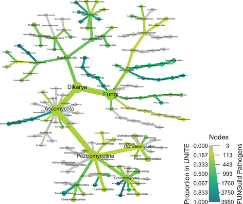
One of the major goals of metabarcoding is to identify the diversity of taxonomic groups in a sample. Taxonomic classification should always be interpreted with caution. There are two major factors that influence classification. First, taxonomic classifications are only as good as the completeness and accuracy of the reference database used for comparing ASVs/OTUs. For example, many of the pathogenic fungi within the FUNGuild database (Nguyen et al. 2016) do not have sequences in UNITE database that are used for taxonomic classification (Fig. 1). Second, many microorganisms have not been cultured or sequenced, and their sequences may not be properly curated or identified in reference databases. Less specialized databases, such as GenBank, can be used, but these are not curated specifically for metabarcoding and may have taxonomic errors or outdated information (Nilsson et al. 2006). Therefore, choice of database is key (Table 1). Hence, if new loci are used for metabarcoding, it may be necessary to assemble and build a high-quality database or risk making unsubstantiated inferences on the taxonomic identities within communities.

Fig. 1 A heat tree generated using the metacoder and taxa (Foster et al. 2018) packages in R that illustrates the proportion of pathogenic species in FUNGuild that have sequences in UNITE for each taxon, based on the MycoBank taxonomic classification. FUNGuild is a database of fungal species with information on their lifestyle (Nguyen et al. 2016). The names of pathogenic species were searched for in the UNITE database, the primary database used for identification of fungi from ITS sequences. Note that most species do not have sequences available in UNITE and many taxa do not have any sequence representing them.

The two methods typically used for querying databases are BLAST (Altschul et al. 1990) and the Naive Bayes Classifier (Wang et al. 2007). When using BLAST, each representative ASV/OTU sequence is searched against a reference database and the taxonomic assignment of alignments are typically used to identify each of the ASVs/OTUs. The percentage of alignment can be quite low due to poor reference database coverage. In addition, BLAST parameters and results should be carefully chosen and interpreted, respectively. It is good practice to set searches and filter results based on percent identity to the query sequence, query coverage, or e-value. Filtering can be used to ignore classifications inferred based on less related hits. There also may be multiple matches of similar quality but with different taxonomic classifications, which is typical for many taxa and loci if the locus used does not confer species-level resolution. This can be somewhat controlled for by considering only top hits to taxonomic ranks that do not disagree with other hits. Without careful parametrization, quality filtering, design, manual/visual interpretation, and validation when needed, it can be difficult to interpret BLAST-based classifications with confidence (Blaxter et al. 2005).

The Naive Bayes Classifier uses a k-mer-based resampling approach to independently assign taxonomic rank for each ASV or OTU (Wang et al. 2007). An example of a tool that uses a Naive Bayes Classifier algorithm is the DADA2 function assignTaxonomy (Callahan et al. 2016). Each assignment is given a score that measures the proportion of bootstrapped resamplings that support the best matching taxonomic assignment. This method avoids many of the complications described for the BLAST-based approach. However, when the Naive Bayes Classifier is used to assign ranks based on a locus with low taxonomic resolution, it is typical to get low confidence classifications at lower taxonomic levels. While this is an accurate result that reflects the limitations of the locus, it may be an unwelcome surprise. For this reason, the Naive Bayes Classifier is not often used with some loci, such as ITS1 for fungal metabarcoding. However taxonomic assignments are made, it is important to use some combination of bootstrap scores, percent identity, alignment coverage, and knowledge about the taxonomic resolution of the locus to estimate the likelihood that assignments are correct. This is especially true when the goal of the analysis is to detect potentially destructive pathogens that might require costly control measures.

Differential taxon abundance techniques

Metabarcoding experiments are often designed to compare the abundance of taxa among samples and associate differences with potential environmental factors. For example, a researcher studying the effects of a fungicide might seek to test if there are any taxa whose abundance decreases relative to a control treatment. Standard statistical tests such as a simple t-test or the Wilcoxon rank-sum test are not appropriate tests when examining the differential abundance of different taxa among samples because the proportional nature of read abundance data violates their assumptions (Lin and Peddada 2020). In metabarcoding, there will be a maximum number of reads sequenced with a given platform in a sequencing run. Therefore, the proportion of reads representing any particular taxon in a sample depends not only on its abundance, but also the abundance of others (McLaren et al. 2019). For example, even if the bacterial load of one species is the same in two samples but one sample has low diversity and the other has high diversity, reads of this conceptual bacterial species may represent 80% and 10%, respectively, of the sequenced DNA reads. Given that this problem is analogous to that of using RNA-Seq datasets to infer differential gene expression, the same methods used for analysis of RNA-Seq reads can be used to infer differential taxon abundance in metabarcoding datasets. Commonly used software packages include DESeq2 (Love et al. 2014), edgeR (Robinson et al. 2010), and ANCOM (Lin and Peddada 2020), which also automatically apply multiple comparison corrections.

Diversity estimation and visualization tools

Researchers using metabarcoding are often interested in testing for differences in community diversity. In this context, ‘community’ refers to a collection of ASVs/OTUs/taxa (referred to as ‘types’ in this section) derived from a single sample. The diversity of a single community or sample is known as alpha diversity and the difference between two communities is known as beta diversity (Jost et al. 2006; Daly et al. 2018). A statistic used to measure diversity is generally referred to as a diversity index. The most common indices only consider the number of types and their abundance, but they vary in how much weight they give to low-abundance types relative to high-abundance types. Assuming the number of types (ASVs/OTUs/taxa) is the same between two communities, a diversity index that incorporates relative abundance will indicate that the community with more equally abundant types (more even) is more diverse. Some indices, such as UniFrac, also consider sequence similarity of types when quantifying diversity (Lozupone and Knight 2005; Lozupone et al. 2011). Programs calculating these indices take as input a phylogenetic tree of all sequences (or infer such a tree from other input) as well as the abundance of each sequence. Communities with more differences between sequences are considered more diverse, assuming the number and abundance of types is the same. The best choice of diversity measure will depend on which aspects of diversity (e.g. number of types, relative abundance of types, similarity of sequences, etc.) are most relevant to the experimental question. For a broad overview of diversity metrices, refer to Table 2. The following paragraphs describe commonly used indices for quantifying alpha and beta diversity, specifying which aspects of diversity each measure.

Table 2. A summary of alpha and beta diversity indices.

	Index	Comparison	Visualization
Alpha diversity
Diversity/abundance	Shannon	ANOVA, Kruskal-Wallis
	Simpson
	Inversed Simpson
Evenness	Shannon
	Pielou
Beta diversity
Dissimilarity: species number & relative abundance	Bray-Curtis	PCA, NDMS, PERMANOVA	Ordination plots, heat trees, scatterplots
Distance: relatedness & phylogenetic distances	UniFrac

There are numerous approaches for estimating alpha diversity and each measures a different aspect of the communities (Chao et al. 2014). The most basic measure is richness which is simply the number of types in a sample. The Shannon entropy index (Shannon 1948) and the inverse Simpson index (Simpson 1949) are both commonly used measures that consider the relative abundance of types, but the Simpson index gives more weight to common taxa than the Shannon entropy index does. Another group of indices measures how even the abundance of types are in each sample regardless of number of types. Pielou’s evenness is an example of this kind of index (Pielou 1966). Some indices also consider phylogenetic relatedness, such as ‘phylogenetic entropy’ (Allen et al. 2009) and ‘taxonomic diversity’ (Warwick and Clarke 1995). Many of these measures can be calculated with the R package vegan (Oksanen 2010). Once the alpha diversity indices of choice are calculated, they can be compared visually by generating boxplots or tested with ANOVA or Kruskal – Wallis statistical tests.

There are also several approaches for calculating beta diversity. Common indices include the Bray – Curtis dissimilarity and a group of related measures called UniFrac (Lozupone and Knight 2005; Lozupone et al. 2011). Bray-Curtis dissimilarity takes into account both the number of species and their relative abundance. Unifrac is notable for incorporating phylogenetic distances between taxa as well. There are also statistics such as the Aitchison distance (Aitchison et al. 2000) that are designed to work with the type of compositional data produced by metabarcoding. Beta diversity values, representing a comparison between two communities, often result in a distance matrix containing values for every pairwise combination of samples. The pairwise nature of beta diversity measures makes them harder to visualize and interpret compared to alpha diversity measures. To overcome this, dimensionality reduction techniques such as non-metric multidimensional scaling (NMDS) or principal component analysis (PCA) are used. These techniques attempt to represent the information contained within the distance matrix of OTU/ASVs as a lower dimension space associated with each sample. These values can then be visualized in a two-dimensional or three-dimensional scatter plot, with data coloured by sample type. Samples with similar communities are then expected to cluster near each other. If experimental group/treatment membership correlates with the similarity of communities, then there will be distinct clusters of samples for each group/treatment. This relationship can be tested statistically for significance using PERMANOVA in the vegan R package (Dixon 2003).

Another method of visualizing taxon abundance and differences among communities is plotting heat trees (Foster et al. 2017). Heat trees are network-like plots derived from taxonomic classifications that use colour and size to display information associated with taxa. The R package metacoder can be used to create heat trees by first creating a taxonomic tree for all OTUs or ASVs observed across all samples based on their classification (Foster et al. 2017). Pairwise community comparisons or other taxon-specific statistics can then be plotted on the tree. Heat trees can show differential abundance using a diverging colour scale as is commonly done in heatmaps. This approach shows information in a taxonomic context, allowing for comparisons across all taxonomic levels unlike traditional stacked bar charts that show abundance at only one taxonomic level.

Towards more accessible and reproducible data

Data associated with a metabarcoding experiment, including raw sequence reads, metadata, OTU/ASV matrices, and taxonomic tables should be deposited into publicly available databases upon completion of a manuscript. To allow for reproducibility, all aspects of the analysis should be described in the materials and methods and scripts shared in appropriate repositories such as Github. In addition, report-generating language extensions, such as R Markdown (Xie et al. 2018, 2020; R Markdown: dynamic documents for R; 2023) or Jupyter Notebooks (Kluyver et al. 2016), can be used to combine the results with the code used to generate them (Kluyver et al. 2016; Xie et al. 2018). The reports rendered in R Markdown or Jupyter can easily be shared as accessible and reproducible workflows in repositories such as GitHub.

Conclusions

Metabarcoding is a powerful tool for plant pathology. It has application in detecting difficult to culture pathogens, surveying ecosystems and asymptomatic plants for pathogens, and revealing the identities of pathogens when traditional methods are inadequate. Still, it remains important to appreciate the limitations of metabarcoding and interpret results accordingly because incorrect taxonomic classifications could mask detection of an important pathogen or lead to an incorrect diagnosis. It is essential to understand sources of error and bias as well as how the locus used impacts the ability to assign taxonomic ranks and identities. While metabarcoding is a helpful pre-screening tool, it is still important to combine the approach with more robust validation methods. It is possible that in the future, the ease of assembly enabled by long reads and decreasing sequencing costs will make PCR-free shotgun metagenomics preferable to metabarcoding. However, shotgun metagenomics requires many more reads and more computational power to characterize communities to the same depth as metabarcoding. This problem is exacerbated when the goal is to target a small fraction of the total DNA in a sample, such as studying endophyte communities in a plant sample or a rare group of organisms in a soil sample dominated by bacteria and fungi. Therefore, it is likely that metabarcoding will remain an important tool for the foreseeable future.

The future is bright for metabarcoding. Its effectiveness is likely to increase as methods using longer read lengths are developed and reference databases expand. Sequencing technologies that produce long reads, such as PacBio and Nanopore, allow for the use of barcodes with more taxonomic resolution (Tedersoo et al. 2021). These methods are being developed and tested now. In addition, continual improvements to analytical packages and advances in statistical tests are making analysis of metabarcoding data easier and more robust. Finally, reference databases are being continuously expanded, increasing the comprehensiveness of organisms that can be identified. The contribution of high-quality sequences from known organisms to reference databases will be crucial for the success of new and existing metabarcoding methods.

Acknowledgments

We thank the Canadian Phytopathological Society for inviting us to present our work at their 2022 annual meeting.

Disclosure statement

No potential conflict of interest was reported by the author(s).

Additional information

Funding

This work was supported by the National Institutes of Food and Agriculture, US Department of Agriculture award 2021-67021-34343 to NJG and JHC, the USDA-ARS CRIS Project 2072-22000-039-00D to NJG; the 2020 CDFA Specialty Block Grant Program Project 45 to NJG and JHC; and the USDA-ARS Floriculture Nursery Initiative research programs to NJG.

References

- Abdala Asbun A, Besseling MA, Balzano S, van Bleijswijk JDL, Witte HJ, Villanueva L, Engelmann JC. 2020. Cascabel: a scalable and versatile amplicon sequence data analysis pipeline delivering reproducible and documented results. Front Genet. 11:489357. doi: 10.3389/fgene.2020.489357.
- Abellan-Schneyder I, Matchado MS, Reitmeier S, Sommer A, Sewald Z, Baumbach J, List M, Neuhaus K. 2021. Primer, pipelines, parameters: issues in 16S rRNA gene sequencing. mSphere. 6(1):e01202–20. doi: 10.1128/mSphere.01202-20.
- Aitchison J, Barceló-Vidal C, Martín-Fernández JA, Pawlowsky-Glahn V. 2000. Logratio analysis and compositional distance. Math Geol. 32(3):271–5. doi: 10.1023/A:1007529726302.
- Allen B, Kon M, Bar-Yam Y. 2009. A new phylogenetic diversity measure generalizing the Shannon index and its application to phyllostomid bats. Am Nat. 174(2):236–243. doi: 10.1086/600101.
- Altschul SF, Gish W, Miller W, Myers EW, Lipman DJ. 1990. Basic local alignment search tool. J Mol Biol. 215(3):403–410. doi: 10.1016/S0022-2836(05)80360-2.
- Anslan S, Bahram M, Hiiesalu I, Tedersoo L. 2017. PipeCraft: flexible open-source toolkit for bioinformatics analysis of custom high-throughput amplicon sequencing data. Mol Ecol Resour. 17(6):e234–e240. doi: 10.1111/1755-0998.12692.
- Anslan S, Mikryukov V, Armolaitis K, Ankuda J, Lazdina D, Makovskis K, Vesterdal L, Schmidt IK, Tedersoo L. 2021. Highly comparable metabarcoding results from MGI-Tech and Illumina sequencing platforms. PeerJ. 9:e12254. doi: 10.7717/peerj.12254.
- Apprill A, McNally S, Parsons R, Weber L. 2015. Minor revision to V4 region SSU rRNA 806R gene primer greatly increases detection of SAR11 bacterioplankton. Aquat Microb Ecol. 75(2):129–137. doi: 10.3354/ame01753.
- Arrigoni E, Antonielli L, Pindo M, Pertot I, Perazzolli M. 2018. Tissue age and plant genotype affect the microbiota of apple and pear bark. Microbial Res. 211:57–68. doi: 10.1016/j.micres.2018.04.00204.002.
- Bastida F, Eldridge DJ, García C, Kenny Png G, Bardgett RD, Delgado-Baquerizo M. 2021. Soil microbial diversity–biomass relationships are driven by soil carbon content across global biomes. IMSE J. 15(7):2081–91. doi: 10.1038/s41396-021-00906-0.
- Beckers B, Op De Beeck M, Weyens N, Boerjan W, Vangronsveld J. 2017. Structural variability and niche differentiation in the rhizosphere and endosphere bacterial microbiome of field-grown poplar trees. Microbiome. 5:1–7. doi: 10.1186/s40168-017-0241-2.
- Bellemain E, Carlsen T, Brochmann C, Coissac E, Taberlet P, Kauserud H. 2010. ITS as an environmental DNA barcode for fungi: an in silico approach reveals potential PCR biases. BMC Microbiol. 10(1):189. doi: 10.1186/1471-2180-10-189.
- Blaxter M, Mann J, Chapman T, Thomas F, Whitton C, Floyd R, Abebe E. 2005. Defining operational taxonomic units using DNA barcode data. Philos T R Soc B. 360(1462):1935–1943. doi: 10.1098/rstb.2005.1725.
- Bohmann K, Elbrecht V, Carøe C, Bista I, Leese F, Bunce M, Yu DW, Seymour M, Dumbrell AJ, Creer S. 2022. Strategies for sample labelling and library preparation in DNA metabarcoding studies. Mol Ecol Resour. 22(4):1231–1246. doi: 10.1111/1755-0998.13512.
- Bolger AM, Lohse M, Usadel B. 2014. Trimmomatic: a flexible trimmer for Illumina sequence data. Bioinformatics. 30(15):2114–2120. doi: 10.1093/bioinformatics/btu170.
- Bolyen E, Rideout JR, Dillon MR, Bokulich NA, Abnet CC, Al-Ghalith GA, Alexander H, Alm EJ, Arumugam M, Asnicar F, et al. 2019. Reproducible, interactive, scalable and extensible microbiome data science using QIIME 2. Nat Biotechnol. 37(8):852–857. doi: 10.1038/s41587-019-0209-9.
- Boutigny A-L, Gautier A, Basler R, Dauthieux F, Leite S, Valade R, Aguayo J, Ioos R, Laval V, Melcher U. 2019. Metabarcoding targeting the EF1 alpha region to assess Fusarium diversity on cereals. PLoS ONE. 14(1):e0207988. doi: 10.1371/journal.pone.0207988.
- Buchner D, Macher T-H, Leese F, Alkan C. 2022. APSCALE: advanced pipeline for simple yet comprehensive analyses of DNA metabarcoding data. Bioinformatics. 38(20):4817–4819. doi: 10.1093/bioinformatics/btac588.
- Bukin YS, Galachyants YP, Morozov I, Bukin S, Zakharenko A, Zemskaya T. 2019. The effect of 16S rRNA region choice on bacterial community metabarcoding results. Sci Data. 6(1):190007. doi: 10.1038/sdata.2019.7.
- Bullington LS, Lekberg Y, Larkin BG. 2021. Insufficient sampling constrains our characterization of plant micro biomes. Sci Rep. 11(1):3645. doi: 10.1038/s41598-021-83153-9.
- Callahan BJ, McMurdie PJ, Holmes SP. 2017. Exact sequence variants should replace operational taxonomic units in marker-gene data analysis. ISME J. 11(12):2639–2643. doi: 10.1038/ismej.2017.119.
- Callahan BJ, McMurdie PJ, Rosen MJ, Han AW, Johnson AJA, Holmes SP. 2016. DADA2: high-resolution sample inference from Illumina amplicon data. Nat Methods. 13(7):581. doi: 10.1038/nmeth.3869.
- Callahan BJ, Wong J, Heiner C, Oh S, Theriot CM, Gulati AS, McGill SK, Dougherty MK. 2019. High-throughput amplicon sequencing of the full-length 16S rRNA gene with single-nucleotide resolution. Nucleic Acids Res. 47(18):e103. doi: 10.1093/nar/gkz569.
- Caporaso JG, Lauber CL, Walters WA, Berg-Lyons D, Lozupone CA, Turnbaugh PJ, Fierer N, Knight R. 2011. Global patterns of 16S rRNA diversity at a depth of millions of sequences per sample. P Natl Acad Sci. 108(supplement_1):4516–4522. doi: 10.1073/pnas.1000080107.
- Chao A, Gotelli NJ, Hsieh T, Sander EL, Ma K, Colwell RK, Ellison AM. 2014. Rarefaction and extrapolation with Hill numbers: a framework for sampling and estimation in species diversity studies. Ecol Monogr. 84(1):45–67. doi: 10.1890/13-0133.1.
- Chen W, Zhang CK, Cheng Y, Zhang S, Zhao H, Casiraghi M. 2013. A comparison of methods for clustering 16S rRNA sequences into OTUs. PLoS ONE. 8(8):e70837. doi: 10.1371/journal.pone.0070837.
- Costello M, Fleharty M, Abreu J, Farjoun Y, Ferriera S, Holmes L, Granger B, Green L, Howd T, Mason T, et al. 2018. Characterization and remediation of sample index swaps by non-redundant dual indexing on massively parallel sequencing platforms. Bmc Genom. 19(1):332. doi:10.1186/s12864-018-4703.
- Daly AJ, Baetens JM, De Baets B. 2018. Ecological diversity: measuring the unmeasurable. Mathematics. 6(7):119. doi: 10.3390/math6070119.
- Davis NM, Proctor DM, Holmes SP, Relman DA, Callahan BJ. 2018. Simple statistical identification and removal of contaminant sequences in marker-gene and metagenomics data. Microbiome. 6(1):226. doi: 10.1186/s40168-018-0605-2.
- De Boer SH, López MM. 2012. New grower-friendly methods for plant pathogen monitoring. Annu Rev Phytopathol. 50(1):197–218. doi: 10.1146/annurev-phyto-081211-172942.
- Dickie IA, Boyer S, Buckley HL, Duncan RP, Gardner PP, Hogg ID, Holdaway RJ, Lear G, Makiola A, Morales SE, et al. 2018. Towards robust and repeatable sampling methods in eDNA-based studies. Mol Ecol Resour. 18(5):940–952. doi:10.1111/1755-0998.12907.
- Di Tommaso P, Chatzou M, Floden EW, Barja PP, Palumbo E, Notredame C. 2017. Nextflow enables reproducible computational workflows. Nat Biotechnol. 35(4):316–319. doi: 10.1038/nbt.3820.
- Dixon P. 2003. VEGAN, a package of R functions for community ecology. J Veg Sci. 14(6):927–930. doi: 10.1111/j.1654-1103.2003.tb02228.x.
- Dopheide A, Xie D, Buckley TR, Drummond AJ, Newcomb RD, Bunce M. 2019. Impacts of DNA extraction and PCR on DNA metabarcoding estimates of soil biodiversity. Methods Ecol Evol. 10(1):120–133. doi: 10.1111/2041-210X.13086.
- Edgar RC. 2010. Search and clustering orders of magnitude faster than BLAST. Bioinformatics. 26(19):2460–2461. doi: 10.1093/bioinformatics/btq461.
- Edgar RC. 2016. UNOISE2: improved error-correction for Illumina 16S and ITS amplicon sequencing. BioRxiv: 081257.
- Edgar RC, Valencia A. 2018. Updating the 97% identity threshold for 16S ribosomal RNA OTUs. Bioinformatics. 34(14):2371–2375. doi: 10.1093/bioinformatics/bty113.
- Edwards RA, Rohwer F. 2005. Viral metagenomics. Nat Rev Microbiol. 3(6):504–510. doi: 10.1038/nrmicro1163.
- Eisenhofer R, Minich JJ, Marotz C, Cooper A, Knight R, Weyrich LS. 2019. Contamination in low microbial biomass microbiome studies: issues and recommendations. Trends Microbiol. 27(2):105–117. doi: 10.1016/j.tim.2018.11.003.
- Escudié F, Auer L, Bernard M, Mariadassou M, Cauquil L, Vidal K, Maman S, Hernandez-Raquet G, Combes S, Pascal G, et al. 2018. FROGS: find, rapidly, OTUs with Galaxy solution. Bioinformatics. 34(8):1287–1294. doi: 10.1093/bioinformatics/btx791.
- Fierer N. 2017. Embracing the unknown: disentangling the complexities of the soil microbiome. Nat Rev Microbiol. 15(10):579–590. doi: 10.1038/nrmicro.2017.87.
- Fiore-Donno AM, Human ZR, Štursová M, Mundra S, Morgado L, Kauserud H, Baldrian P, Bonkowski M. 2022. Soil compartments (bulk soil, litter, root and rhizosphere) as main drivers of soil protistan communities distribution in forests with different nitrogen deposition. Soil Biol Biochem. 168:108628. doi: 10.1016/j.soilbio.2022.108628.
- Fisher MC, Henk DA, Briggs CJ, Brownstein JS, Madoff LC, McCraw SL, Gurr SJ. 2012. Emerging fungal threats to animal, plant and ecosystem health. Nature. 484(7393):186–194. doi: 10.1038/nature10947.
- Foster ZSL, Albornoz FE, Fieland VJ, Larsen MM, Jones FA, Tyler BM, Nguyen HDT, Burgess TI, Riddell C, Voglmayr H, et al. 2022. A new oomycete metabarcoding method using the rps10 gene. Phytobiomes J. 6(3):214–226. doi:10.1094/PBIOMES-02-22-0009-R.
- Foster ZSL, Chamberlain S, Grünwald NJ. 2018. Taxa: an R package implementing data standards and methods for manipulation of taxonomic data. F1000Res. 7:272. doi: 10.12688/f1000research.14013.2 2.
- Foster ZS, Sharpton TJ, Grünwald NJ, Poisot T. 2017. Metacoder: an R package for visualization and manipulation of community taxonomic diversity data. PLoS Comput Biol. 13(2):e1005404. doi: 10.1371/journal.pcbi.1005404.
- Fu L, Niu B, Zhu Z, Wu S, Li W. 2012. CD-HIT: accelerated for clustering the next-generation sequencing data. Bioinformatics. 28(23):3150–3152. doi: 10.1093/bioinformatics/bts565.
- Gweon HS, Oliver A, Taylor J, Booth T, Gibbs M, Read DS, Griffiths RI, Schonrogge K, Bunce M. 2015. PIPITS: an automated pipeline for analyses of fungal internal transcribed spacer sequences from the Illumina sequencing platform. Methods Ecol Evol. 6(8):973–980. doi: 10.1111/2041-210X.12399.
- Jalili V, Afgan E, Gu Q, Clements D, Blankenberg D, Goecks J, Taylor J, Nekrutenko A. 2020. The Galaxy platform for accessible, reproducible and collaborative biomedical analyses: 2020 update. Nucleic Acids Res. 48(W1):W395–W402. doi: 10.1093/nar/gkaa434.
- Janda JM, Abbott SL. 2007. 16S rRNA gene sequencing for bacterial identification in the diagnostic laboratory: pluses, perils, and pitfalls. J Clin Microbiol. 45(9):2761–2764. doi: 10.1128/JCM.01228-07.
- Jiang H, Lei R, Ding SW, Zhu S. 2014. Skewer: a fast and accurate adapter trimmer for next-generation sequencing paired-end reads. BMC Bioinform. 15:1–2. doi: 10.1186/1471-2105-15-182.
- Jost L. 2006. Entropy and diversity. Oikos. 113(2):363–375. doi: 10.1111/j.2006.0030-1299.14714.x.
- Kemp BM, Smith DG. 2005. Use of bleach to eliminate contaminating DNA from the surface of bones and teeth. Forensic Sci Int. 154(1):53–61. doi: 10.1016/j.forsciint.2004.11.017.
- Kluyver T, Ragan-Kelley B, Pérez F, Granger B, Bussonnier M, Frederic J, Kelley K, Hamrick J, Grout J, Corlay S, et al. 2016. Jupyter notebooks – a publishing format for reproducible computational workflows. In: Loizides F Scmidt B, editors. Positioning and power in academic publishing: players, agents and agendas. IOS Press; pp. 87–90. https://eprints.soton.ac.uk/403913/.
- Kõljalg U, Nilsson RH, Abarenkov K, Tedersoo L, Taylor AFS, Bahram M, Bates ST, Bruns TD, Bengtsson-Palme J, Callaghan TM, et al. 2013. Towards a unified paradigm for sequence-based identification of fungi. Mol Ecol. 22(21):5271–5277. doi:10.1111/mec.12481.
- Laforest-Lapointe I, Messier C, Kembel SW. 2016. Tree phyllosphere bacterial communities: exploring the magnitude of intra-and inter-individual variation among host species. PeerJ. 24:e2367. doi: 10.7717/peerj.2367.
- Latz MA, Grujcic V, Brugel S, Lycken J, John U, Karlson B, Andersson A, Andersson AF. 2022. Short‐and long‐read metabarcoding of the eukaryotic rRNA operon: evaluation of primers and comparison to shotgun metagenomics sequencing. Mol Ecol Resour. 22(6):2304–18. doi: 10.1111/1755-0998.13623.
- Lin H, Peddada SD. 2020. Analysis of compositions of microbiomes with bias correction. Nat Commun. 11:3514. doi: 10.1038/s41467-020-17041-7.
- Loos D, Zhang L, Beemelmanns C, Kurzai O, Panagiotou G. 2021. DAnIEL: a user-friendly web server for fungal ITS amplicon sequencing data. Front Microbiol. 12. doi: 10.3389/fmicb.2021.720513.
- Love MI, Huber W, Anders S. 2014. Moderated estimation of fold change and dispersion for RNA-seq data with DESeq2. Genome Biol. 15(12):550. doi: 10.1186/s13059-014-0550-8.
- Lozupone C, Knight R. 2005. UniFrac: a new phylogenetic method for comparing microbial communities. Appl Environ Microbiol. 71(12):8228–8235. doi: 10.1128/AEM.71.12.8228-8235.2005.
- Lozupone C, Lladser ME, Knights D, Stombaugh J, Knight R. 2011. UniFrac: an effective distance metric for microbial community comparison. ISME J. 5(2):169–172. doi: 10.1038/ismej.2010.133.
- Maidak BL, Olsen GJ, Larsen N, Overbeek R, McCaughey MJ, Woese CR. 1996. The ribosomal database project (RDP). Nucleic Acids Res. 24(1):82–85. doi: 10.1093/nar/24.1.82.
- Martin M. 2011. Cutadapt removes adapter sequences from high-throughput sequencing reads. EMBnet J. 17(1):10–12. doi: 10.14806/ej.17.1.200.
- McLaren MR, Willis AD, Callahan BJ. 2019. Consistent and correctable bias in metagenomic sequencing experiments. Elife. 8:e46923. doi: 10.7554/eLife.46923.
- McNear DH Jr. 2013. The rhizosphere-roots, soil and everything in between. Nature Ed Knowl. 4(3):1.
- Mölder F, Jablonski KP, Letcher B, Hall MB, Tomkins-Tinch CH, Sochat V, Forster J, Lee S, Twardziok SO, Kanitz A, et al. 2021. Sustainable data analysis with Snakemake. F1000Res. 10:33. doi: 10.12688/f1000research.29032.2.
- Munoz‐Ucros J, Zwetsloot MJ, Cuellar‐Gempeler C, Bauerle TL, Wandrag E. 2021. Spatiotemporal patterns of rhizosphere microbiome assembly: from ecological theory to agricultural application. J Appl Ecol. 58(5):894–904. doi: 10.1111/1365-2664.13850.
- Nguyen NH, Song Z, Bates ST, Branco S, Tedersoo L, Menke J, Schilling JS, Kennedy PG. 2016. Funguild: an open annotation tool for parsing fungal community datasets by ecological guild. Fungal Ecol. 20:241–248. doi: 10.1016/j.funeco.2015.06.006.
- Nichols RV, Vollmers C, Newsom LA, Wang Y, Heintzman PD, Leighton M, Green RE, Shapiro B. 2018. Minimizing polymerase biases in metabarcoding. Mol Ecol Resour. 18(5):927–939. doi: 10.1111/1755-0998.12895.
- Nilsson RH, Anslan S, Bahram M, Wurzbacher C, Baldrian P, Tedersoo L. 2019. Mycobiome diversity: high-throughput sequencing and identification of fungi. Nat Rev Microbiol. 17(2):95–109. doi: 10.1038/s41579-018-0116-y.
- Nilsson RH, Ryberg M, Kristiansson E, Abarenkov K, Larsson K-H, Kõljalg U, Fairhead C. 2006. Taxonomic reliability of DNA sequences in public sequence databases: a fungal perspective. PLoS ONE. 1(1):e59. doi: 10.1371/journal.pone.0000059.
- Oksanen J 2010. Vegan: community ecology package. http://CRAN.R-project.org/package=vegan.
- Öpik M, Vanatoa A, Vanatoa E, Moora M, Davison J, Kalwij JM, Reier Ü, Zobel M. 2010. The online database MaarjAM reveals global and ecosystemic distribution patterns in arbuscular mycorrhizal fungi (Glomeromycota). New Phytol. 188(1):223–241. doi: 10.1111/j.1469-8137.2010.03334.x.
- Özkurt E, Fritscher J, Soranzo N, DYK N, Davey RP, Bahram M, Hildebrand F. 2022. LotuS2: an ultrafast and highly accurate tool for amplicon sequencing analysis. Microbiome. 10(1):176. doi: 10.1186/s40168-022-01365-1.
- Palmer JM, Jusino MA, Banik MT, Lindner DL. 2018. Non-biological synthetic spike-in controls and the AMPtk software pipeline improve mycobiome data. PeerJ. 6:e4925. doi: 10.7717/peerj.4925.
- Parada AE, Needham DM, Fuhrman JA. 2016. Every base matters: assessing small subunit rRNA primers for marine microbiomes with mock communities, time series and global field samples. Environ Microbiol. 18(5):1403–1414. doi: 10.1111/1462-2920.13023.
- Paulson JN, Stine OC, Bravo HC, Pop M. 2013. Differential abundance analysis for microbial marker-gene surveys. Nat Methods. 10(12):1200–1202. doi: 10.1038/nmeth.2658.
- Pervaiz ZH, Contreras J, Hupp BM, Lindenberger JH, Chen D, Zhang Q, Wang C, Twigg P, Saleem M. 2020. Root microbiome changes with root branching order and root chemistry in peach rhizosphere soil. Rhizosphere. 16:100249. doi: 10.1016/j.rhisph.2020.100249.
- Pielou EC. 1966. The measurement of diversity in different types of biological collections. J Theor Biol. 13:131–144. doi: 10.1016/0022-5193(66)90013-0.
- Piombo E, Abdelfattah A, Droby S, Wisniewski M, Spadaro D, Schena L. 2021. Metagenomics approaches for the detection and surveillance of emerging and recurrent plant pathogens. Microorganisms. 9(1):188. doi: 10.3390/microorganisms9010188.
- Prince AM, Andrus L. 1992. PCR: how to kill unwanted DNA. Biotechniques. 12(3):358–360.
- Qiu X, Wu L, Huang H, McDonel PE, Palumbo AV, Tiedje JM, Zhou J. 2001. Evaluation of PCR-generated chimeras, mutations, and heteroduplexes with 16S rRNA gene-based cloning. Appl Environ Microb. 67(2):880–887. doi: 10.1128/AEM.67.2.880-887.2001.
- Quast C, Pruesse E, Yilmaz P, Gerken J, Schweer T, Yarza P, Peplies J, Glöckner FO. 2013. The SILVA ribosomal RNA gene database project: improved data processing and web-based tools. Nucleic Acids Res. 41(Database issue):D590–D596. doi: 10.1093/nar/gks1219.
- Quince C, Walker AW, Simpson JT, Loman NJ, Segata N. 2017. Shotgun metagenomics, from sampling to analysis. Nat Biotechnol. 35(9):833–844. doi: 10.1038/nbt.3935.
- Richter-Heitmann T, Eickhorst T, Knauth S, Friedrich MW, Schmidt H. 2016. Evaluation of strategies to separate root-associated microbial communities: a crucial choice in rhizobiome research. Front Microbiol. 7. doi: 10.3389/fmicb.2016.00773.
- Riit T, Tedersoo L, Drenkhan R, Runno-Paurson E, Kokko H, Anslan S. 2016. Oomycete-specific ITS primers for identification and metabarcoding. MycoKeys. 14:17–30. doi: 10.3897/mycokeys.14.9244.
- R Markdown: dynamic documents for R. 2023. https://github.com/rstudio/rmarkdown.
- Robertson BL, Brown JA, McDonald T, Jaksons P. 2013. BAS: balanced acceptance sampling of natural resources. Biometrics. 69(3):776–784. doi: 10.1111/biom.12059.
- Robinson MD, McCarthy DJ, Smyth GK. 2010. edgeR: a Bioconductor package for differential expression analysis of digital gene expression data. Bioinformatics. 26(1):139–140. doi: 10.1093/bioinformatics/btp616.
- Rognes T, Flouri T, Nichols B, Quince C, Mahé F. 2016. VSEARCH: a versatile open source tool for metagenomics. PeerJ. 4:e2584. doi: 10.7717/peerj.2584.
- Salipante SJ, Kawashima T, Rosenthal C, Hoogestraat DR, Cummings LA, Sengupta DJ, Harkins TT, Cookson BT, Hoffman NG, Löffler FE. 2014. Performance comparison of Illumina and Ion Torrent next-generation sequencing platforms for 16S rRNA-based bacterial community profiling. Appl Environ Microbiol. 80(24):7583–7591. doi: 10.1128/AEM.02206-14.
- Salter SJ, Cox MJ, Turek EM, Calus ST, Cookson WO, Moffatt MF, Turner P, Parkhill J, Loman NJ, Walker AW. 2014. Reagent and laboratory contamination can critically impact sequence-based microbiome analyses. BMC Biol. 12(1):87. doi: 10.1186/s12915-014-0087-z.
- Sanzani SM, Destri Nicosia MG L, Faedda R, Cacciola SO, Schena L. 2014. Use of quantitative PCR detection methods to study biocontrol agents and phytopathogenic fungi and oomycetes in environmental samples. J Phytopathol. 162(1):1–13. doi: 10.1111/jph.12147.
- Sapkota R, Jørgensen LN, Nicolaisen M. 2017. Spatiotemporal variation and networks in the mycobiome of the wheat canopy. Front Plant Sci. 2(8):1357. doi: 10.3389/fpls.2017.01357.
- Sapkota R, Nicolaisen M. 2015. An improved high throughput sequencing method for studying oomycete communities. J Microbiol Meth. 110:33–39. doi: 10.1016/j.mimet.2015.01.013.
- Sapp M, Lewis E, Moss S, Barrett B, Kirk S, Elphinstone JG, Denman S. 2016. Metabarcoding of bacteria associated with the acute oak decline syndrome in England. Forests. 7(5):95. doi: 10.3390/f7050095.
- Schloss PD. 2020. Reintroducing mothur: 10 years later. McBain AJ, editor. Appl Environ Microbiol. 86(2):e02343–19. doi:10.1128/AEM.02343-19.
- Schloss PD, Westcott SL, Ryabin T, Hall JR, Hartmann M, Hollister EB, Lesniewski RA, Oakley BB, Parks DH, Robinson CJ, et al. 2009. Introducing mothur: open-source, platform-independent, community-supported software for describing and comparing microbial communities. Appl Environ Microbiol. 75(23):7537–7541. doi: 10.1128/AEM.01541-09.
- Schrader C, Schielke A, Ellerbroek L, Johne R. 2012. PCR inhibitors–occurrence, properties and removal. J Appl Microbiol. 113(5):1014–1026. doi: 10.1111/j.1365-2672.2012.05384.x.
- Shannon CE. 1948. A mathematical theory of communication. Bell Syst Tech J. 27(3):379–423. doi: 10.1002/j.1538-7305.1948.tb01338.x.
- Simpson EH. 1949. Measurement of diversity. Naturen. 163(4148):688–688. doi: 10.1038/163688a0.
- Sow A, Brévault T, Benoit L, Chapuis M-P, Galan M, Coeur D’acier A, Delvare G, Sembène M, Haran J. 2019. Deciphering host-parasitoid interactions and parasitism rates of crop pests using DNA metabarcoding. Sci Rep. 9(1):1–12. doi: 10.1038/s41598-019-40243-z.
- Straub D, Blackwell N, Langarica-Fuentes A, Peltzer A, Nahnsen S, Kleindienst S. 2020. Interpretations of environmental microbial community studies are biased by the selected 16S rRNA (gene) amplicon sequencing pipeline. Front Microbiol. 11:550420. doi: 10.3389/fmicb.2020.550420.
- Sylla J, Alsanius BW, Krüger E, Reineke A, Strohmeier S, Wohanka W. 2013. Leaf microbiota of strawberries as affected by biological control agents. Phytopathology. 103(10):1001–1011. doi: 10.1094/PHYTO-01-13-0014-R.
- Taberlet P, Coissac E, Pompanon F, Brochmann C, Willerslev E. 2012. Towards next-generation biodiversity assessment using DNA metabarcoding. Mol Ecol. 21(8):2045–2050. doi: 10.1111/j.1365-294X.2012.05470.x.
- Tedersoo L, Albertsen M, Anslan S, Callahan B, Druzhinina IS. 2021. Perspectives and benefits of high-throughput long-read sequencing in microbial ecology. Appl Environ Microbiol. 87(17):e00626–21. doi: 10.1128/AEM.00626-21.
- Tedersoo L, Bahram M, Zinger L, Nilsson RH, Kennedy PG, Yang T, Anslan S, Mikryukov V. 2022. Best practices in metabarcoding of fungi: from experimental design to results. Mol Ecol. 31(10):2769–2795. doi: 10.1111/mec.16460.
- Tedersoo L, Lindahl B. 2016. Fungal identification biases in microbiome projects. Env Microbiol Rep. 8(5):774–779. doi: 10.1111/1758-2229.12438.
- Theil S, Rifa E. 2021. rANOMALY: AmplicoN wOrkflow for microbial community anaLysis. F1000Res. 10(7): doi: 10.12688/f1000research27268.1.
- U’Ren JM, Riddle JM, Monacell JT, Carbone I, Miadlikowska J, Arnold AE. 2014. Tissue storage and primer selection influence pyrosequencing-based inferences of diversity and community composition of endolichenic and endophytic fungi. Mol Ecol Resour. 14(5):1032–1048. doi: 10.1111/1755-0998.12252.
- Vasar M, Davison J, Neuenkamp L, Sepp S-K, Young JPW, Moora M, Öpik M. 2021. User-friendly bioinformatics pipeline gDAT (graphical downstream analysis tool) for analysing rDNA sequences. Mol Ecol Resour. 21(4):1380–1392. doi: 10.1111/1755-0998.13340.
- Wagner MR, Lundberg DS, Del Rio TG, Tringe SG, Dangl JL, Mitchell-Olds T. 2016. Host genotype and age shape the leaf and root microbiomes of a wild perennial plant. Nat Commun. 7(1):12151. doi: 10.1038/ncomms12151.
- Wang Q, Garrity GM, Tiedje JM, Cole JR. 2007. Naive Bayesian classifier for rapid assignment of rRNA sequences into the new bacterial taxonomy. Appl Environ Microbiol. 73(16):5261–5267. doi: 10.1128/AEM.00062-07.
- Warwick RM, Clarke KR. 1995. New ‘biodiversity’ measures reveal a decrease in taxonomic distinctness with increasing stress. Mar Ecol Prog Ser. 129:301–305. doi: 10.3354/meps129301.
- White T, Bruns T, Lee S, Taylor J, Innis M, Gelfand D, Sninsky J. 1990. Amplification and direct sequencing of fungal ribosomal RNA genes for phylogenetics. In: Innis MA, Gelfand DH, Sninsky JJ, White TJ, editors. PCR protocols: a guide to methods and applications. Vol. 31. London (UK): Academic Press; pp. 315–322.
- Xie Y, Allaire JJ, Grolemund G. 2018. R Markdown: the definitive guide. Boca Raton (FL): Chapman and Hall/CRC. https://bookdown.org/yihui/rmarkdown.
- Xie Y, Dervieux C, Riederer E. 2020. R Markdown cookbook. Boca Raton (FL): Chapman and Hall/CRC. https://bookdown.org/yihui/rmarkdown-cookbook.
- Zafeiropoulos H, Viet HQ, Vasileiadou K, Potirakis A, Arvanitidis C, Topalis P, Pavloudi C, Pafilis E. 2020. PEMA: a flexible pipeline for environmental DNA metabarcoding analysis of the 16S/18S ribosomal RNA, ITS, and COI marker genes. GigaScience. 9(3):giaa022. doi: 10.1093/gigascience/giaa022.
- Zhang J, Kobert K, Flouri T, Stamatakis A. 2014. PEAR: a fast and accurate Illumina paired-end reAd mergeR. Bioinformatics. 30(5):614–620. doi: 10.1093/bioinformatics/btt593.