Instrument Validity Tests With Causal Forests

Abstract

Assumptions that are sufficient to identify local average treatment effects (LATEs) generate necessary conditions that allow instrument validity to be refuted. The degree to which instrument validity is violated, however, probably varies across subpopulations. In this article, we use causal forests to search and test for such local violations of the LATE assumptions in a data-driven way. Unlike previous instrument validity tests, our procedure is able to detect local violations. We evaluate the performance of our procedure in simulations and apply it in two different settings: parental preferences for mixed-sex composition of children and the Vietnam draft lottery.

KEYWORDS:

• Causal forest
• Instrument validity
• Local average treatment effect
• Specification tests
• Treatment effects

1 Introduction

Producing credible estimates of causal effects in empirical research often entails a heavy reliance on instrumental variables (IVs). IVs, however, have to meet strong assumptions to be valid. Discussions about threats to these identifying assumptions and approaches to checking their robustness constitute a crucial part of many empirical articles. Recently, Kitagawa (2015), Huber and Mellace (2015), and Mourifié and Wan (2017) developed tests that allow the validity of IVs to be refuted based on necessary conditions in the data. These conditions are generated by the joint assumptions sufficient to identify local average treatment effects (LATEs), namely the exclusion restriction, randomization/unconfoundedness, and monotonicity (Imbens and Angrist 1994; Angrist, Imbens, and Rubin 1996). The unifying idea across these three tests is that, given a treatment status, the estimated density of compliers must be nonnegative at any point in the distribution of the outcome variable; compliers comprise the unobserved subpopulation of individuals whose treatment status is causally affected by the instrument.

The concept underlying our article is that the degree to which the LATE assumptions are violated may vary across subpopulations that can be defined by observed characteristics. For example, a direct effect of the instrument on the outcome variable may be large in a relatively small subpopulation but, in the entire population, watered down to the point at which it can no longer be detected by existing tests. By reformulating the necessary conditions into a form similar to that employed to learn the sign of treatment effects, we are able to leverage recent progress in using machine learning to estimate heterogeneous treatment effects. This heterogeneity is conceptually restricted to nonnegative values if the LATE assumptions hold, but may take on negative values otherwise.

In recent years, a growing body of research has used machine learning to estimate heterogeneous treatment effects (Tian et al. 2014; Wager and Athey 2018; Athey, Tibshirani, and Wager 2019; Künzel et al. 2019; Nie and Wager 2019, among others). Our test proceeds in three steps. In the spirit of subgroup testing, we use shallow regression trees (Breiman et al. 1984) to split the sample along covariate values. Some of these splits form subgroups, which are promising for finding violations of the LATE assumptions. We apply a simple selection procedure to identify these. Then, we use the double machine learning framework from Chernozhukov et al. (2018) combined with causal forests developed by Wager and Athey (2018) and Athey, Tibshirani, and Wager (2019) to estimate the magnitude of the violations in these promising subgroups. Lastly, we test for local violations of the LATE assumptions using Bonferroni-corrected critical values. Finding violations in at least one subgroup casts doubt on the instrument, because we cannot rule out further undetected violations. Our proposed test procedure can be easily implemented with existing software packages. Additionally, we provide the R package LATEtest.

We consider a setup with a binary (endogenous) treatment and a binary IV. There are several examples in this framework: for instance, the Vietnam draft lottery (Angrist 1990), the preference for mixed-sex children (Angrist and Evans 1998), or the Oregon health insurance experiment (Finkelstein et al. 2012). When we apply our data-driven procedure to detect local violations of IV validity, we have to assume that the instrument is randomized (or at least unconfounded conditional on covariates). Randomization (or unconfoundedness) itself is therefore not testable with our procedure. However, randomization (or unconfoundedness) is often fulfilled by design in applied work (for instance, in the Vietnam draft lottery or in the Oregon health insurance experiment), while the most controversial assumption is the exclusion restriction and to some extent also monotonicity. We thus have applications in mind in which the researcher is interested in testing the exclusion restriction and/or monotonicity.

The existing test procedures are, ceteris paribus, more powerful when the overall share of compliers in the entire population is low, that is, the instrument is weak on average. However, applied researchers often rely on strong instruments to avoid issues associated with weak IVs (Bound, Jaeger, and Baker 1995), and because a larger share of compliers may deliver a causal effect with greater external validity. Our test procedure is more powerful when the share of compliers is low within a subpopulation. That is, our test can have more power asymptotically than existing tests even if the instrument turns out to be strong on average. The proposed approach also has advantages over simply using existing IV validity tests within arbitrarily defined covariate subgroups. It automatically chooses the covariates and covariate values to partition on, with honest splitting safeguarding the researcher from an overfitting bias. Researchers can, therefore, credibly demonstrate that they have extensively searched for violations of key identifying assumptions.

This article contributes to the recent and fast growing literature on adapting machine learning tools to the needs of applied economists who wish to estimate causal effects and detect and characterize the heterogeneity of these. One strand of the literature uses tree and forest algorithms to estimate the heterogeneity of treatment effects (Asher et al. 2016; Athey and Imbens 2016; Wager and Athey 2018; Athey, Tibshirani, and Wager 2019). Belloni et al. (2012), Belloni, Chernozhukov, and Hansen (2014b), and Chernozhukov, Hansen, and Spindler (2015) presented methods based on the least absolute shrinkage and selection operator (Lasso, Tibshirani 1996) for inference in high-dimensional settings where there may be many possible instrument or control variables relative to the number of observations. See also Belloni, Chernozhukov, and Hansen (2014a) for an overview. Knaus, Lechner, and Strittmatter (2020) used Lasso-type estimators to detect treatment effect heterogeneity in job search programs. In the presence of instruments that violate the exclusion restriction, Kang et al. (2016) and Windmeijer et al. (2019) used the Lasso to select valid IVs in linear models. Wager et al. (2016), Bloniarz et al. (2016), and Athey, Imbens, and Wager (2018) improved the efficiency of average treatment effect estimates in randomized experiments with Lasso-based balancing.

The rest of this article proceeds as follows. In the next section, we briefly revisit the testable implications of IV validity. Section 3 describes our procedure to detect, select and test local violations of IV validity. In Sections 4 and 5, we provide results from a simulation study and apply the test to real data. Section 6 concludes.

2 (Local) Violations of LATE

Let the observed outcome Y have support $\mathcal{Y}$ and the endogenous treatment have status $D\in \{0,1\}$, where D = 1 indicates treatment, and the binary instrument $Z\in \{0,1\}$. The potential outcomes and treatments are denoted with Y^dz and D^z, where $d,z\in \{0,1\}$. Following Imbens and Angrist (1994) and Abadie (2003), three assumptions are sufficient to identify LATEs in this setup.

Assumption A1.

(Exclusion restriction): $Y^{d1}=Y^{d0}=Y^d$ for $d\in \{0,1\}$ wp1.

Assumption A2.a.

(Randomization):$$(Y^{11},Y^{10},Y^{01},Y^{00},D^1,D^0)\perp Z.$$

Assumption A2.

b. (Unconfoundedness):$$(Y^{11},Y^{10},Y^{01},Y^{00},D^1,D^0)\perp Z|X.$$

Assumption A3.

(Monotonicity): $D^1\ge D^0$ or $D^1\le D^0$ wp1.

Assumption A1 rules out a direct effect of the instrument on the potential outcomes. Assumption A2.a assumes that Z is jointly independent of the potential outcomes and treatments. In many applications, Assumption A2.a will hold only when conditioning on a set of predetermined covariates X. In this case, Assumption A2.b replaces Assumption A2.a. Assumption A3 rules out the existence of defiers. Without loss of generality, we assume $D^1\ge D^0$ in the remainder of this article, that is, the instrument is to create an incentive to take up the treatment, and we assume that this is known a priori to the researcher. Our arguments would hold symmetrically for negative monotonicity (i.e., $D^1\le D^0$).

Let ${\mathcal{B}}_{\mathcal{Y}}$ be a collection of Borel sets generated from $\mathcal{Y}$. Imbens and Rubin (1997) showed that, under Assumptions A1–A3, it must hold for every $J\in {\mathcal{B}}_{\mathcal{Y}}$ that$$\begin{array}{c}P(Y\in J,D=1|Z=1)-P(Y\in J,D=1|Z=0)\\ \hspace{1em}=P(Y^1\in J,C),\\ P(Y\in J,D=0|Z=0)-P(Y\in J,D=0|Z=1)\\ \hspace{1em}=P(Y^0\in J,C).\end{array}$$

Since the share of compliers (C) has to be nonnegative at every point in the distribution of Y, the following inequalities must hold(2.1) $$P(Y\in J,D=1|Z=1)-P(Y\in J,D=1|Z=0)\ge 0,$$(2.1) (2.2) $$P(Y\in J,D=0|Z=0)-P(Y\in J,D=0|Z=1)\ge 0.$$(2.2)

Balke and Pearl (1997) and Heckman and Vytlacil (2005) also discussed these testable implications. Kitagawa (2015) used a variance-weighted Kolmogorov–Smirnov-type statistic to test (2.1) and (2.2). Mourifié and Wan (2017) rewrite (2.1) and (2.2) as conditional moment inequalities (conditional on Y = y) and then apply the intersection bounds approach of Chernozhukov, Lee, and Rosen (2013). Huber and Mellace (2015) relaxed Assumptions A1 and A2 to hold only in expectation because this is sufficient to identify average effects. Kitagawa (2015, Proposition 1.1) and Mourifié and Wan (2017, Theorem 1) established that (2.1) and (2.2) are sharp, in the sense that they are the strongest testable implications of Assumptions A1–A3 given the available data. Laffers and Mellace (2017) proved that the inequalities proposed by Huber and Mellace (2015) are the strongest testable implications when Assumptions A1 and A2 hold only in expectation.

The inequalities (2.1) and (2.2) must hold at any point x in the covariate space $\mathcal{X}$ as well(2.3) $$\begin{array}{c}P(Y\in J,D=1|Z=1,X=x)\\ \hspace{1em}-P(Y\in J,D=1|Z=0,X=x)\ge 0,\end{array}$$(2.3) (2.4) $$\begin{array}{c}P(Y\in J,D=0|Z=0,X=x)\\ \hspace{1em}-P(Y\in J,D=0|Z=1,X=x)\ge 0.\end{array}$$(2.4)

Conditioning on X can be helpful in several ways. For illustration, if we only impose randomization/unconfoundedness, we can derive from (2.3)$$\begin{array}{c}P(Y\in J,D=1|Z=1,X=x)-P(Y\in J,D=1|Z=0,X=x)\\ \hspace{1em}=P(Y^{11}\in J|C,X=x)P(C|X=x)\\ \mathrm{\hspace{1em}}\mathrm{\hspace{1em}}-P(Y^{10}\in J|F,X=x)P(F|X=x)\\ \mathrm{\hspace{1em}}\mathrm{\hspace{1em}}+P(Y^{11}\in J|A,X=x)P(A|X=x)\\ \mathrm{\hspace{1em}}\mathrm{\hspace{1em}}-P(Y^{10}\in J|A,X=x)P(A|X=x)\ge 0,\end{array}$$where A, C, and F denote always-takers, compliers, and defiers, respectively. First, the proportion of compliers within some covariate cell, $P(C|X=x)$, might be lower than in the full sample. Second, the fraction of defiers might be overrepresented or exist only in certain covariate cells. In both cases, local violations of Assumption A3 can be detected more easily when we condition on those cells. Third, the direct effect of the instrument might be stronger for some subpopulations, making it easier to find local violations of Assumption A1 when we condition on X.

Kitagawa (2015), Huber and Mellace (2015), and Mourifié and Wan (2017) also applied their tests within covariate cells. However, how to form these cells so that they make finding violations of the LATE assumptions more likely is an open question, in particular when covariates are continuous. Arbitrarily defining subgroups is inefficient. A further problem is the potentially large dimensionality of X, which makes implementation of the above tests for all x infeasible. Therefore, we propose a data-driven way to find and test local violations of IV validity.

3 A Local IV Validity Test

Let $(Y_i,D_i,Z_i,X_i)$ be iid observations for $i=1,\dots ,n$. Define for any $J\in {\mathcal{B}}_{\mathcal{Y}}$ the pseudo variables$$Q_{J,d,i}:=\{\begin{array}{c}{Q}_{J,1,i}=-1\{Y_i\in J\}{D}_i\hfill \\ Q_{J,0,i}=1\{Y_i\in J\}(1-D_i)\hfill \end{array}$$for $d\in \{0,1\}$. The necessary conditions stated in Equations (2.3)(2.3) $$\begin{array}{c}P(Y\in J,D=1|Z=1,X=x)\\ \hspace{1em}-P(Y\in J,D=1|Z=0,X=x)\ge 0,\end{array}$$(2.3) and (2.4)(2.4) $$\begin{array}{c}P(Y\in J,D=0|Z=0,X=x)\\ \hspace{1em}-P(Y\in J,D=0|Z=1,X=x)\ge 0.\end{array}$$(2.4) can be interpreted as learning the sign of the treatment effect of Z on $Q_{J,d}$ conditional on covariates. Note that the assignment of the instrument is now the “treatment.” We first use a causal forest (CF) to estimate conditional average treatment effects (CATEs). Second, we grow shallow trees to search for subgroups in the covariate space, in which we observe heterogeneity in the CATEs. These shallow trees summarize the heterogeneity signals in the CATE, and allow for easy implementation and visualization of our local IV test. Third, we discuss a procedure to select the promising subgroups, in which we may exhibit potential violations. Finally, we test whether the group average treatment effects in these promising subgroups are incompatible with the LATE assumptions. In the following, we describe our test procedure in more detail. Additionally, Appendix A in the supplementary materials gives further information regarding the implementation of our test in R and collects the main steps of our procedure in pseudo code.

3.1 Estimating Heterogeneous Treatment Effects

Let(3.1) $${\tau }_{J,d}(x)=\mathbb{E}\left[Q_{J,d,i}\right|Z_i=1,X_i=x]-\mathbb{E}[Q_{J,d,i}|Z_i=0,X_i=x]$$(3.1) be the CATE of Z on $Q_{J,d}$ at X = x. Under Assumptions A1–A3, ${\tau }_{J,d}(x)\le 0$ must hold for every combination of J, d, and x. Due to our definition of $Q_{J,d}$, positive signs of ${\tau }_{J,d}(x)$ now point to violations of the LATE assumptions. For all possible combinations of J and d, we regress out the marginal effects that X has on $Q_{J,d}$ and Z using random forests (Breiman 2001) to account for the potential confounding, and use the residuals to estimate ${\tau }_{J,d}(x)$ with causal forests. Wager and Athey (2018) and Athey, Tibshirani, and Wager (2019) derived pointwise asymptotic normality of the causal forest estimator ${\widehat{\tau }}_{J,d}(x)$ under certain regularity assumptions. The assumptions to establish causality are

Assumption

CF1. $(Q_{J,d}^1,Q_{J,d}^0)\perp Z|X$.

Assumption

CF2. For some $ϵ>0$ it holds$$ϵ<\mathrm{P}(Z=1|X=x)<1-ϵ.$$

Note that Assumption CF1 is implicitly part of Assumption A2 as the pseudo outcomes are functions of Y^dz and D^z. Therefore, randomization or unconfoundedness—depending on the application we have in mind—is not testable with our procedure. Neither (A1) nor (A3) are, however, necessary to estimate a CF and can thus be tested with our procedure. Assumption CF2 assumes overlap, meaning that the instrument must not be deterministic in X. An empirical example in which this assumption may be violated is the twin birth instrument (Rosenzweig and Wolpin 1980; Angrist and Evans 1998; Farbmacher, Guber, and Vikström 2018). Twinning strongly depends on maternal age (X) and is a very rare (if not even impossible) event if the expectant mother is very young.

To assess the magnitude of the potential violations of the LATE assumptions, we use the augmented inverse probability weighted scores from Robins, Rotnitzky, and Zhao (1994)(3.2) $$\begin{array}{c}{\widehat{\Gamma }}_{J,d,i}:={\widehat{\tau }}_{J,d}^{(-i)}(X_i)+\frac{Z_i-{\widehat{e}}^{(-i)}(X_i)}{{\widehat{e}}^{(-i)}(X_i)(1-{\widehat{e}}^{(-i)}(X_i))}\hfill \\ \hspace{1em}\times \left(Q_{J,d,i}-{\widehat{\mu }}_{J,d}^{(-i)}(X_i)-(Z_i-{\widehat{e}}^{(-i)}(X_i)){\widehat{\tau }}_{J,d}^{(-i)}(X_i)\right),\hfill \end{array}$$(3.2) where ${\widehat{\tau }}_{J,d}^{(-i)}(X_i),{\widehat{e}}^{(-i)}(X_i)$, and ${\widehat{\mu }}_{J,d}^{(-i)}(X_i)$ denote leave-one-out estimates of ${\tau }_{J,d}(x),e(x)=\mathrm{P}(Z_i=1|X_i=x)$, and ${\mu }_{J,d}(x)=\mathbb{E}(Q_{J,d,i}|X_i=x)$, respectively. Leave-one-out (or out-of-bag) estimates are obtained without using the ith observation. We average ${\widehat{\Gamma }}_{J,d,i}$ over all observations i that fall into certain subgroups, which we define in a data-driven way as discussed in the next section.

3.2 Detecting and Selecting Promising Subgroups

We use regression trees as a data-driven approach to partition the data along observable covariates. Trees have already been used to perform subgroup analysis in the context of heterogeneous effects (e.g., Su et al. 2009; Athey and Imbens 2016). We grow a single tree on each score ${\widehat{\Gamma }}_{J,d}$ using the classification and regression tree (CART) algorithm (Breiman et al. 1984). The CART algorithm is essentially a data mining tool that recursively adds axis-aligned splits to the tree. It will split the sample at the covariate value that delivers the largest heterogeneity between the newly formed subgroups. We denote the resulting tree structure by ${\Pi }_{J,d}$, which is a collection of terminal and nonterminal nodes—the terminal nodes are also called leaves. The leaves partition the covariate space into a set of rectangles. The CART algorithm is greedy in the sense that it tries to improve the splitting criterion only at the next split, without considering possible future splits. The splitting ends after certain criteria are met. An important parameter here is the user-defined minimum number of observations ultimately required to be in each leaf.

Growing a tree deeply uncovers more heterogeneity and may make it more likely to find violations of the LATE assumptions. A deeper tree, however, also implies smaller sample sizes within the leaves, leading to noisier estimates. A classic solution to solve this bias-variance trade-off is to penalize tree size proportional to a constant, which is determined via K-fold cross-validation. This is called pruning. In the first step, we grow a complete tree without any early stopping criteria other than a minimum leaf size, which can lead to a quite large and complex tree structure. In a second step, we prune this tree using 10-fold cross-validation applying the optimal complexity parameter. Pruning gives us a set of relevant subgroups, that is, groups that potentially exhibit heterogeneity in ${\tau }_{J,d}(x)$ independent of its sign.

We are, however, particularly interested in finding sign heterogeneity in ${\tau }_{J,d}(x)$. Under Assumptions A1–A3, ${\tau }_{J,d}(x)$ can vary only between –1 and 0 for any x. However, if the IV is invalid, ${\tau }_{J,d}(x)$ can vary between –1 and 1. Therefore, local violations of the LATE assumptions may induce observable heterogeneity in the sign of ${\tau }_{J,d}(x)$. For illustrative purposes, consider testing Assumption A3 separately. This is a special case of our testing procedure, which reduces to finding sign heterogeneity in the first stage effect and testing for the presence of defiers. In this case, we let J cover the whole domain of Y, that is, $Q_1=-D$, and Q₀ is redundant. Then, the absolute value of ${\tau }_1(x)=-E[D^1-D^0|X=x]$ measures the conditional average treatment effect of Z on D, which reflects the local fraction of compliers or defiers. Finding positive CATEs would imply that, for some observations, the instrument actually creates a disincentive to take up the treatment, which violates the monotonicity assumption. Note that identifying the LATE may still be possible in such a setting under additional assumptions (de Chaisemartin 2017).

The following selection procedure aims to find the “most” promising subgroups within the relevant ones. We regard a subgroup as promising if we can exhibit potential violations of the LATE assumptions within it, that is, subgroups in which the CATE is potentially positive. We only use these selected subgroups in the local IV test to increase its power. To ensure the validity of the test, we perform this selection on the training sample. First, we select only the leaves of the pruned trees. If the violations are sufficiently strong, the pruned tree will partition the sample accordingly. Second, we exclude leaves in which the CATE turns out to be clearly negative. Such leaves point to a sizeable fraction of compliers, which makes it hard to detect violations in this subgroup. Finally, we compare each leaf with its left or right pair and use only the leaf side that exhibits a larger average treatment effect. We give additional details about this selection procedure in Appendix A in the supplementary materials.

3.3 Testing for Local Violations of IV Validity

We use honest estimation to prevent a bias from overfitting (see, e.g., Athey and Imbens 2016). That is, one randomly chosen part of the sample, called the training sample, is used to build the tree while the remaining sample, called the estimation sample, is used to estimate (group) average treatment effects, which are ultimately used for our local IV test. Instead of training and estimation, we will call the two random halves of the full sample S^A and S^B, and we will swap the roles of the samples to alleviate the inefficiency of the sample splitting (following Chernozhukov et al. 2018). For each combination of J and d, we grow the trees ${\Pi }_{J,d}^{S^A}$ and ${\Pi }_{J,d}^{S^B}$, respectively. Due to the sample swapping and as $d\in \{0,1\}$, we build four times as many pruned trees as we use intervals to discretize Y.

Consider the expectation of ${\Gamma }_{d,i}$ for a given partition$$\begin{array}{c}{\zeta }_{J,d,l}^A=\mathbb{E}\left[{\Gamma }_{J,d,i}|X_i\in L_l(x;{\Pi }_{J,d}^{S^B})\right],\\ {\zeta }_{J,d,l}^B=\mathbb{E}\left[{\Gamma }_{J,d,i}|X_i\in L_l(x;{\Pi }_{J,d}^{S^A})\right],\end{array}$$where $L_l(x;{\Pi }_{J,d})$ denotes the lth element of the set of selected leaves of the tree ${\Pi }_{J,d}$. The expectations within these partitions are then estimated in sample S^A when the tree has been obtained in sample S^B, and vice versa. In the remainder of the article, we keep the sample swapping procedure implicit.

We collect the moments of the selected leaves over all combinations of J and d in $\zeta =({\zeta }^A,{\zeta }^B)$. Positive elements of ζ are local violations of the LATE assumptions. Therefore, we test the following null hypothesis$$\begin{array}{cc}{H}_0:{\zeta }_j\le 0\hfill & \text{for}\text{all}j=1,\dots ,p\hfill \\ H_1:{\zeta }_j>0\hfill & \text{for}\text{some}j=1,\dots ,p,\hfill \end{array}$$where $p=\left|\zeta \right|$. Rejecting the null means that the LATE assumptions are violated in at least one subpopulation. Finding a violation in any subpopulation casts doubt on the IV validity in the entire population because we cannot rule out further violations in other subpopulations.

For ease of notation, let t_j denote the jth variable that we use to estimate the moment ζ_j from a total of p moments. Furthermore, let ${\widehat{\zeta }}_j=\frac{1}{n_j}\sum _i{t}_{ij}$ denote the sample mean of the jth variable and ${\widehat{\sigma }}_j^2=\frac{1}{n_j-1}\sum _i(t_{ij}-{\widehat{\zeta }}_j{)}^2$ its sample variance with n_j the sample size within leaf j. We consider the test statistic(3.3) $$T=\underset{1\le j\le p}{\text{max}}\frac{\sqrt{n_j}{\widehat{\zeta }}_j}{{\widehat{\sigma }}_j}.$$(3.3)

Under the H₀ it must hold that$$T\le \underset{1\le j\le p}{\text{max}}\frac{\sqrt{n_j}({\widehat{\zeta }}_j-{\zeta }_j)}{{\widehat{\sigma }}_j},$$hence, finding an upper bound for the $(1-\alpha )$ quantile of $\sqrt{n_j}({\widehat{\zeta }}_j-{\zeta }_j)/{\widehat{\sigma }}_j$ is sufficient to keep the actual size of the test at or below α. Using a Bonferroni correction for multiple testing, a critical value for T is(3.4) $$c(\alpha )={\Phi }^{-1}(1-\alpha /p).$$(3.4)

If one is interested not only in the global null hypothesis, but additionally in obtaining the subgroups that violate the LATE assumptions, the Bonferroni–Holm correction is more powerful.

To obtain our asymptotic result, we will rely on recent findings from the double machine learning framework. Observe that, as described in Athey and Wager (2017), the estimator from (3.2) can be interpreted as(3.5) $$\begin{array}{c}{\widehat{\Gamma }}_{J,d,i}:={\widehat{m}}_{J,d}^{(-k)}(X_i,1)-{\widehat{m}}_{J,d}^{(-k)}(X_i,0)\hfill \\ +\frac{Z_i-{\widehat{e}}^{(-k)}(X_i)}{{\widehat{e}}^{(-k)}(X_i)(1-{\widehat{e}}^{(-k)}(X_i))}\left(Q_{J,d,i}-{\widehat{m}}_{J,d}^{(-k)}(X_i,Z_i)\right),\hfill \\ e(x)=P(Z_i=1|X_i=x),\hfill \\ m_{J,d}(x,z)=\mathbb{E}\left[Q_{J,d}|Z=z,X_i=x\right],\hfill \end{array}$$(3.5) which aligns with the double machine learning framework introduced by Chernozhukov et al. (2018). Here, $m_{J,d}(·)$ and $e(·)$ are unknown nuisance functions. In their Theorem 5.1, they establish that the mean of the estimates ${\widehat{\Gamma }}_{J,d,i}$ is asymptotically Gaussian and efficient, as long as the nuisance estimates ${\widehat{m}}_{J,d}^{(-k)}(·)$ and ${\widehat{e}}^{(-k)}(·)$ converge sufficiently fast and are determined by crossfitting, which we indicate by ${}^{(-k)}$ here. Adapted to our testing problem, the following assumptions are needed to derive asymptotic results.

Assumption

T1. For all J, d and every selected leaf l, it holds$$\begin{array}{c}P\left(X\in L_l(x;{\Pi }_{J,d})\right)\ge c>0\text{and}\\ \mathbb{E}\left[{\left(Q_{J,d}-m_{J,d}(X,Z)\right)}^2|X\in L_l(x;{\Pi }_{J,d})\right]\ge c>0,\end{array}$$where c is a generic constant independent of n.

Assumption

T2. The nuisance functions are estimated via K-fold crossfitting, and with probability no less than $1-o(1)$ it holds

1. $\left|\right|{\widehat{e}}^{(-k)}(X)-\frac{1}{2}|{|}_{P,\infty }\le \frac{1}{2}-ϵ$,

2. $\max (||{\widehat{e}}^{(-k)}(X)-e(X)|{|}_{P,2}$,

${\max }_{J,d}\left|\right|{\widehat{m}}_{J,d}^{(-k)}(X,Z)-m_{J,d}(X,Z)|{|}_{P,2})\le {\delta }_n{n}^{-1/4}$, where ${\delta }_n=o({\hspace{0.17em}\text{log}\hspace{0.17em}}^{-1}(n))$.

Assumption T1 ensures that the number of observations in the subgroups defined by the selected leaves of the pruned trees increases with the sample size. Moreover, it assumes that the pseudo outcome variable is nondeterministic in each leaf given X and Z. The first part of Assumption T2 assumes that the estimates of the propensity score are bounded away from zero and one, which is a standard assumption in the literature. The second part of Assumption T2 states that, with probability converging to one, all nuisance components are $o\left(n^{-\frac{1}{4}}\right)$ consistent with respect to the L₂-error. This rate is much weaker than the standard rate of $o\left(n^{-\frac{1}{2}}\right)$ due to the so-called Neyman orthogonality or double robustness property of the estimator. In principle, other estimators than random forests (e.g., from Kernel regressions) can be used for the nuisance functions, as long as they fulfill Assumption T2. Moreover, Assumption T2 can be weakened at the expense of a more complicated notation. For a detailed discussion of the convergence rates and sharpness of the conditions, see Chernozhukov et al. (2016, 2018) and Athey and Wager (2017).

The following proposition shows that the probability of rejecting H₀—although being true—does not exceed α asymptotically when we use $c(\alpha )$ as the critical value.

Proposition 1.

Suppose that Assumptions CF1, CF2, T1, and T2 hold, then we have under the H₀ $$P(T>c(\alpha ))\le \alpha +o(1).$$

Proof

. We directly obtain Proposition 1 by relying on Theorem 5.1 from Chernozhukov et al. (2018). The corresponding conditions stated in their Assumption 5.1 have to be satisfied for each subgroup. Our Assumption CF1 implies their Assumption 5.1(a). The first part of our Assumption T1 ensures that the number of observations within all subgroups is O(n), with probability converging to one. Further, the second part of Assumption T1 is equivalent to their Assumption 5.1(d). Assumptions 5.1(b) and 5.1(e) hold because $\left|Q_{J,d}\right|\le 1$ and 5.1(c) is implied by CF2. Lastly, (i) of 5.1(f) is directly implied by $\left|Q_{J,d}\right|\le 1$ and our Assumption T2. The proposition then follows by the union bound.

We derive the subgroups from the leaves of the pruned regression trees after applying our selection procedure described in Section 3.2. If there is no heterogeneity in the CATE, the pruned trees will not split the sample, or splits will occur due to noise only. If the sign of ${\tau }_d(x)$ is negative everywhere but its magnitude is heterogeneous over covariates, then splits may occur even under H₀ but only a few (or even none) of them will turn out to be “promising.” In case the set of hypotheses turns out to be empty (e.g., due to a very strong instrument), we report a test based on the root nodes of the pruned trees. Note that the number of subgroups that can be tested is bounded by Assumption T1.

The pointwise normality of the causal forest estimates could also be used to test for violations of the LATE assumptions at prespecified points in the covariate space. Alternatively, one could rely on uniform confidence bands for ${\tau }_d(x)$. There exists a vast literature on confidence bands for nonparametric functions (Bickel and Rosenblatt 1973; Konakov and Piterbarg 1984; Li 1989; Hall and Horowitz 2013, among others) mostly building on kernel or local polynomial methods. Due to the curse of dimensionality, the performance is reliable up to at most p = 3. Since the number of covariates used to ensure unconfoundedness is usually not that small, most of these methods are not applicable in economics. Lee, Okui, and Whang (2017) developed uniform confidence bands for the average treatment effect conditional on a small ($\le$3) subset of covariates, implying that one would still need to select the promising covariates beforehand. Additionally, they assume parametric specifications for the propensity score and for the remaining covariates to avoid the curse of dimensionality. By using random forests, we can avoid such strong structural assumptions. As a result, in our procedure, the number of covariates can be relatively large although not high-dimensional. To use random forests in high-dimensions, modifications to the algorithm and an assumption of sparsity are needed (Wager and Walther 2015).

4 Simulations

To test the finite sample performance of our new procedure, we run several Monte Carlo simulations. Process 1 simulates a randomized experiment similar to that of Huber and Mellace (2015). While in process 1 Assumption A2.a holds, process 2 simulates a setting in which the instrument is unconfounded (i.e., Assumption A2.b holds). Process 2 uses an easy propensity score of the instrument Z and strong confounding of D. In both processes, we use the same function for Y, which also depends on the covariates X:$$\begin{array}{c}Y=D+{\gamma }_{x}Z+\sum _{k=1}^{3}0.3X_k+u\\ \text{where}{X}_k\sim N(0,1)\text{and}(u,v)\sim N\left(0,\left(\begin{array}{cc}1& 0.3\\ 0.3& 1\end{array}\right)\right)\end{array}$$

Table

Process 1 (randomized):	Process 2 (unconfounded):
$D=1\{{\alpha }_{x}Z+v\}$	$D=1\{b+{\alpha }_{x}Z+v\}$
$Z\sim \text{Bernoulli}(0.5)$	$Z=1\left\{{\sum }_{k=1}^{3}0.2X_k+w\right\}$
	where $b=0.5\hspace{0.17em}\text{log}\hspace{0.17em}(1+e^{X_1+X_2+X_3})$
	and $w\sim N(0,1)$

For both processes, we use different values of γ_x and α_x:

• DGP0 (exogenous but uninformative IV): ${\gamma }_x=0,{\alpha }_x=0$

• DGP1 (exogenous and relevant IV): ${\gamma }_x=0,{\alpha }_x=0.20$

• DGP2 (local violation of monotonicity, defiers exist in subpopulation):$${\gamma }_x=0,{\alpha }_x=\{\begin{array}{cc}-0.75\hfill & \text{if}\mathrm{}{X}_1<{\Phi }^{-1}(0.15)\hfill \\ 0.40\hfill & \text{otherwise}\hfill \end{array}$$

• DGP3 (local violation of exclusion restriction):$${\gamma }_x=\{\begin{array}{cc}1.25& \text{if}\mathrm{}{X}_2<{\Phi }^{-1}(0.15)\\ 0& \text{otherwise}\end{array},{\alpha }_x=0.20$$

• DGP4 (global violation of exclusion restriction):$${\gamma }_x=0.5,{\alpha }_x=0.20$$

• DGP5 (global violation of exclusion restriction but with sign heterogeneity):$${\gamma }_x=\{\begin{array}{cc}0.50\hfill & \text{if}\mathrm{}{X}_3<{\Phi }^{-1}(0.5)\hfill \\ -0.50\hfill & \text{otherwise}\hfill \end{array},{\alpha }_x=0.20$$

DGP0 allows us to verify the control of the nominal test size. There are no compliers in this setting and, therefore, the moment inequalities are binding (i.e., ${\zeta }_j=0$ for all $j=1,\dots ,p$). DGP1 represents the case in which the instrument is not only exogenous but also relevant. In this case, the values of ζ_j are all supposed to be negative. The stronger the instrument is, the more conservative the test will be. In DGP1, the choice of ${\alpha }_x=0.2$ leads to a complier share of roughly 8%. DGP2 models a local violation of monotonicity. The local share of compliers or defiers is given by $\Phi (|{\alpha }_x|)-\Phi (0)$, which multiplied by the size of the subpopulation gives the average share of compliers or defiers in the population. DGP2 leads to an average share of defiers in the population of roughly 4.1%, which are hidden in the covariate space. The average complier share is more than three times as large (13.2%), which makes it hard to refute the LATE assumptions with tests based on the entire sample. DGP3 corresponds to a local violation of the exclusion restriction, while DGP4 and DGP5 globally violate it.

Table 1 shows rejection frequencies for both processes with 1000 replications. The sample size is 3000. We discretize Y into four intervals using an equidistant grid from the minimum to the maximum value of Y. We compare our procedure with Kitagawa’s (2015) test, Mourifié and Wan’s (2017) test, and Huber and Mellace’s (2015) mean and full independence test. We find for both processes that our procedure does not overreject the null hypothesis of no violation of the LATE assumptions at the 5% nominal level (DGP0). Note that the rejection frequency in DGP0 under process 2 (i.e., the instrument is only valid conditional on X) would be 0.296 if we did not regress out the effects that X has on $Q_{J,d}$ and Z. This is, therefore, a crucial step if the instrument is confounded. As expected, the test procedure is conservative if compliers exist and there are no violations of the LATE assumptions (DGP1)—this is in line with the results from Kitagawa’s (2015) test, Mourifié and Wan’s (2017) test, and Huber and Mellace’s (2015) test.

Table 1 Simulation results.

	FGK	K	MW	HM
Process 1
DGP0 (exog but uninformative)	0.036	0.060	0.060	–
DGP1 (exog and relevant)	0.009	0.005	0.007	0.000
DGP2 (local defiers)	0.749	0.005	0.006	0.000
DGP3 (local direct effects)	0.743	0.057	0.066	0.002
DGP4 (global direct effects)	0.907	0.980	0.923	0.980
DGP5 (global direct effects, varying signs)	0.593	0.006	0.003	0.000
Process 2
DGP0 (exog but uninformative)	0.036
DGP1 (exog and relevant)	0.002
DGP2 (local defiers)	0.658
DGP3 (local direct effects)	0.767
DGP4 (global direct effects)	0.972
DGP5 (global direct effects, varying signs)	0.716

NOTE: This table displays rejection frequencies (based on 1000 replications) for significance level of 5% and n = 3000. FGK refers to our test, K to Kitagawa’s (2015) test, MW to Mourifié and Wan (2017), and HM to Huber and Mellace’s (2015) test based on full independence using Chen and Szroeter’s (2014) smooth indicator method with tuning parameters as defined in Section 3 of Huber and Mellace (2015). Huber and Mellace’s (2015) test based on mean independence performs worse in our setting with respect to size and power and is, therefore, not reported. For the FGK test we regress out the marginal effects that X has on $Q_{J,d}$ and Z using random forests.

Under DGP2, the monotonicity assumption is violated only in a certain area of the covariate space. Consequently, we expect that splitting the sample by covariates leads to a strong improvement in test power. Indeed, our procedure has distinctly larger power than the alternative tests in this setting. In case of DGP3, a local violation of the exclusion restriction, our procedure again clearly outperforms the alternatives. When the violation of the exclusion restriction is global (DGP4), the existing tests perform better than our procedure. This is to be expected, because splitting the data by covariates cannot improve the precision of our test but honest splitting of the sample leads to a lower sample size available for estimation. However, if the global violation of the exclusion restriction actually has different signs in local areas of the covariate space, then our test can again perform better than existing ones. In DGP5 we illustrate this by the extreme case of completely opposite direct effects.

In Appendix B in the supplementary materials, we shed some light on the choice of the number of intervals and on the effectiveness of the selection step. Moreover, we employ different methods to account for multiple testing.

5 Applications

In this section, we apply our procedure to two widely used IVs, namely parental preferences for mixed-sex composition of children (Angrist and Evans 1998) and the Vietnam draft lottery (Angrist 1990). The Vietnam draft lottery is an IV that is randomized by design and, therefore, Assumption A2.a holds. There are several studies that use the draft lottery to estimate the causal effect of Vietnam-era military service on civilian earnings, schooling, disability status, or health later in life (see, e.g., Angrist 1990; Angrist, Chen, and Frandsen 2010; Angrist and Chen 2011; Angrist, Chen, and Song 2011). We are interested in the literature investigating the effect of military service on schooling. Angrist and Chen (2011) argued that schooling gains can be attributed to the use of the GI Bill, which made generous schooling benefits available to veterans. This is an important channel of a causal effect of military service on schooling. A potential direct effect of the lottery on schooling, however, arises due to deferments, which, among other reasons, were issued to men who were still attending school. Card and Lemieux (2001) showed that draft avoidance led to a rise in the college enrollment rates of young men. This additional schooling might lead to a violation of the exclusion restriction.

The second application builds on the observation that some parents prefer a mixed-sex composition of their children. Angrist and Evans (1998) proposed using the occurrence of same-sex siblings as an IV for the number of children. Rosenzweig and Wolpin (2000) discussed several reasons why this IV may be invalid. Huber (2015) was the first to test the validity of the LATE assumptions in this setting. He finds no violation in the full sample and very few violations across 22 arbitrarily chosen subgroups and concludes that the IV’s validity in these data cannot be refuted. Our test procedure can be seen as a flexible extension of Table 1 in Huber (2015) or of Section VII in Bisbee et al. (2017), in which we derive the promising subgroups in a data-driven way.

5.1 Results With Original Outcomes

In the first application, we use data from an extract of the 1979 and 1981–1985 March Current Population Survey (CPS) (see Angrist and Krueger 1992, for more details about the data). We consider the 1970 draft lottery, held on December 1969, which affected men born in the period 1944–1950. Since the rate of conscriptions dropped considerably after June 1971, most men who obtained deferments in 1970 (for instance, due to additional schooling) could permanently avoid military service (Card and Lemieux 2001). The Vietnam draft lottery randomly assigned a number from 1 to 366 to men born in this cohort based on their date of birth. The numbers determined the order of the call for conscription, starting with the smallest number. At some point during the year, the Selective Service announced a maximum lottery number that would be called. For instance, the ceiling was 195 in the 1970 lottery. Note that there are some concerns regarding the randomization of the 1970 lottery (see, e.g., Fienberg 1971; Deuchert, Huber, and Schelker 2019). In this application, Y measures education (no college, some college, college), D is veteran status and Z indicates whether the individual’s date of birth led to a lottery number lower than 200, which considerably increased the risk of conscription. We use age, indicators for ethnicity, region dummies, and the year of the survey as covariates. Table 2 shows the test results for this application. All tests (including our test) do not reject the null hypothesis.

Table 2 Test results of the validity tests for the Vietnam draft IV.

	p	T	$c(\alpha )$	p-value
FGK	6	1.49	2.39	0.412
Kitagawa (2015) test				1.000
H&M (2015) full independence				1.000
H&M (2015) mean independence				1.000

NOTE: Data extract from 1979 and 1981–1985 March CPS. Sample size is 20,606.

The sample in the second application consists of married and unmarried mothers aged 21–35 years with at least two children as recorded in the 1980 U.S. census. In this application, Y is the logarithm of annual labor income, Z indicates a same-sex composition of the first two children, and D is an indicator of having more than two children at the time of the census. We use mother’s age in 1980, age at first birth, educational attainment (three levels) and ethnicity as covariates. The upper panel of Table 3 shows the test results for this application. All tests (incl. our test) do not reject the null hypothesis.

Table 3 Test results of the validity tests for the sibling sex IV.

	p	T	$c(\alpha )$	p-value
Original outcome
FGK	20	2.28	2.81	0.228
Kitagawa (2015) test				1.000
H&M (2015) full independence				0.999
H&M (2015) mean independence				1.000
Synthetic outcome
FGK	24	9.08	2.87	0.000
Kitagawa (2015) test				1.000
H&M (2015) full independence				0.999
H&M (2015) mean independence				1.000

NOTE: Data from 1980 U.S. census. Sample size is 220,502. Mourifié and Wan (2017) test is based on a random subsample of 26,342 observations due to computational constraints. It does not reject at the 10% level for both outcomes. We discretize Y into four intervals using an equidistant grid from the minimum to the maximum value of Y. To allow for a faster computation of our test, we use a subsample fraction equal to 0.05 when we grow the random forests (for the orthogonalization) and the causal forests. Moreover, we set the minbucket parameter of rpart to 1600 when we build the pruned trees.

5.2 Results With Synthetic Outcomes

As reported in the previous section, we do not find local violations of the LATE assumptions using the original outcome Y. To further illustrate the performance of our test procedure in a real application, we add a local direct effect of Z to Y. The direct effect is rather small (1/4 of the SD of Y) and applies only to a small subgroup of mothers in the 1980 U.S. census data (3.4% of the sample, i.e., 7513 observations), which makes it hard to find in the full sample,$$Y_{\text{syn}}=Y+1/4{\widehat{\sigma }}_{Y}Z\mathrm{}1\{\text{age}<25\}\mathrm{}1\{\text{educ}=\text{HS}\}.$$

The mean of the outcome variable is essentially unchanged ($\overline{Y}=8.939$ and ${\overline{Y}}_{\text{syn}}=8.944$) since the manipulated subgroup is rather small. The mean in the manipulated subgroup rises from 8.53 to 8.69. Since we choose where the direct effect is located in the covariate space, we can check whether different tests in fact succeed in recovering it.

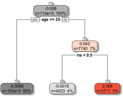
The lower panel of Table 3 shows the test results for the synthetic outcome. Our test clearly rejects the null hypothesis while the p-values of the existing tests are unchanged compared to the results in the upper panel. A traditional subgroup analysis would clearly help them to reject the null hypothesis but cannot be performed since the location of the violation is oracle knowledge. Our data-driven subgroup testing, however, successfully finds the synthetic violation as illustrated in Figure 1, which shows the pruned regression tree leading to the maximum t-statistic.

Fig. 1 Data from 1980 U.S. census (synthetic outcome). Pruned regression tree leading to the maximum t-statistic. The first value in every leaf indicates the effect heterogeneity in the training sample. Positive values indicate violations of the null hypothesis, which still need to be confirmed in the estimation sample. The second line shows the absolute and relative size of each leaf. The text beneath the leaf shows the variable and value on which the leaf was split next.

6 Conclusion

Using IVs to identify LATEs is common in empirical research. In studies that do so, however, the validity of instruments is a point of debate. Fortunately, the LATE framework generates empirically testable implications for instrument validity. In this article, we propose a machine learning based approach to perform IV validity tests in a data-driven way. In the spirit of subgroup testing, our procedure uses the CART algorithm to split the sample along covariate values. Some of these splits form promising subgroups, which can be used to test for local violations of IV validity. We use causal forests to estimate the magnitude of the violations in these subgroups. Our approach can be easily implemented using existing software packages. We provide an R package (LATEtest) and apply our test to two widely used IVs, namely parental preferences for mixed-sex composition of children and the Vietnam draft lottery. In line with the previous literature, we do not find violations of the LATE assumptions in either application.

Our procedure is subject to some restrictions, which offer promising avenues for future research. First, it requires the presence of covariates that are unaffected by the treatment and the IV. The test results are sensitive to the set of covariates we have available. Second, we follow the literature and use an equidistant grid to discretize the outcome variable into a finite number of arbitrarily chosen sets. This could lead to some estimated negative densities not being detected because they can average out with nearby positive densities of compliers in the same set. The literature about scan statistics may make our and the existing tests more powerful by providing a way to find these intervals in a data-driven manner as well (see, e.g., Walther 2010). Third, we need to conduct honest splitting to avoid bias from adaptive searching for violations: one half of the sample is used to build pruned trees while the other half is used to estimate the magnitude of the violations. Although we switch the roles of the samples, doing so reduces the number of observations we can use for testing. Fourth, while detecting promising subgroups with pruned trees allows us to interpret and visualize the source of violations easily, it may not be necessary. A particularly interesting topic of future research will be to test whether the estimates of a causal forest are positive at any point of its support.

Acknowledgments

Helpful comments were provided by Martin Huber, Heinrich Kögel, Romuald Méango, Giovanni Mellace, Martin Spindler, Frank Windmeijer, and seminar participants at Konstanz, London, Odense, the IAAE annual meeting Montréal, the Bank of England conference on modeling with big data and machine learning, and the workshop on causal machine learning in St. Gallen. We thank Christina Nießl for excellent research assistance.

Supplementary Materials

Appendix A gives further information regarding the implementation of our test in R and collects the main steps of our procedure in pseudo code. Appendix B sheds light on the choice of the number of intervals and on the effectiveness of the selection step.

Additional information

Funding

We acknowledge support from the International Doctoral Program “Evidence-Based Economics” of the Elite network of Bavaria and the German Research Foundation (DFG) grant 431701914.

References

- Abadie, A. (2003), “Semiparametric Instrumental Variable Estimation of Treatment Response Models,” Journal of Econometrics, 113, 231–263.
- Angrist, J. D. (1990), “Lifetime Earnings and the Vietnam Era Draft Lottery: Evidence From Social Security Administrative Records,” American Economic Review, 80, 313–336.
- Angrist, J. D., and Chen, S. H. (2011), “Schooling and the Vietnam-Era GI Bill: Evidence From the Draft Lottery,” American Economic Journal: Applied Economics, 3, 96–118.
- Angrist, J. D., Chen, S. H., and Frandsen, B. R. (2010), “Did Vietnam Veterans Get Sicker in the 1990s? The Complicated Effects of Military Service on Self-Reported Health,” Journal of Public Economics, 94, 824–837.
- Angrist, J. D., Chen, S. H., and Song, J. (2011), “Long-Term Consequences of Vietnam-Era Conscription: New Estimates Using Social Security Data,” American Economic Review, 101, 334–338.
- Angrist, J. D., and Evans, W. N. (1998), “Children and Their Parents’ Labor Supply: Evidence From Exogenous Variation in Family Size,” American Economic Review, 88, 450–477.
- Angrist, J. D., Imbens, G. W., and Rubin, D. B. (1996), “Identification of Causal Effects Using Instrumental Variables,” Journal of the American Statistical Association, 91, 444–455.
- Angrist, J. D., and Krueger, A. B. (1992), “Estimating the Payoff to Schooling Using the Vietnam-Era Draft Lottery,” NBER Working Paper No. 4067.
- Asher, S., Nekipelov, D., Novosad, P., and Ryan, S. P. (2016), “Classification Trees for Heterogeneous Moment-Based Models,” NBER Working Paper No. 22976.
- Athey, S., and Imbens, G. (2016), “Recursive Partitioning for Heterogeneous Causal Effects,” Proceedings of the National Academy of Sciences of the United States of America, 113, 7353–7360.
- Athey, S., Imbens, G. W., and Wager, S. (2018), “Approximate Residual Balancing: Debiased Inference of Average Treatment Effects in High Dimensions,” Journal of the Royal Statistical Society, Series B, 80, 597–623.
- Athey, S., Tibshirani, J., and Wager, S. (2019), “Generalized Random Forests,” The Annals of Statistics, 47, 1148–1178.
- Athey, S., and Wager, S. (2017), “Efficient Policy Learning,” arXiv no. 1702.02896.
- Balke, A., and Pearl, J. (1997), “Bounds on Treatment Effects From Studies With Imperfect Compliance,” Journal of the American Statistical Association, 92, 1171–1176.
- Belloni, A., Chen, D., Chernozhukov, V., and Hansen, C. (2012), “Sparse Models and Methods for Optimal Instruments With an Application to Eminent Domain,” Econometrica, 80, 2369–2429.
- Belloni, A., Chernozhukov, V., and Hansen, C. (2014a), “High-Dimensional Methods and Inference on Structural and Treatment Effects,” Journal of Economic Perspectives, 28, 29–50.
- Belloni, A., Chernozhukov, V., and Hansen, C. (2014b), “Inference on treatment Effects After Selection Among High-Dimensional Controls,” Review of Economic Studies, 81, 608–650.
- Bickel, P., and Rosenblatt, M. (1973), “Two-Dimensional Random Fields,” in Multivariate Analysis—III, ed. P. R. Krishnaiah, Amsterdam: Elsevier, pp. 3–15.
- Bisbee, J., Dehejia, R., Pop-Eleches, C., and Samii, C. (2017), “Local Instruments, Global Extrapolation: External Validity of the Labor Supply–Fertility Local Average Treatment Effect,” Journal of Labor Economics, 35, S99–S147.
- Bloniarz, A., Liu, H., Zhang, C.-H., Sekhon, J. S., and Yu, B. (2016), “Lasso Adjustments of Treatment Effect Estimates in Randomized Experiments,” Proceedings of the National Academy of Sciences of the United States of America, 113, 7383–7390.
- Bound, J., Jaeger, D. A., and Baker, R. M. (1995), “Problems With Instrumental Variables Estimation When the Correlation Between the Instruments and the Endogenous Explanatory Variable Is Weak,” Journal of the American Statistical Association, 90, 443–450.
- Breiman, L. (2001), “Random Forests,” Machine Learning, 45, 5–32.
- Breiman, L., Friedman, J., Olshen, R. A., and Stone, C. J. (1984), Classification and Regression Trees, Boca Raton, FL: CRC Press.
- Card, D., and Lemieux, T. (2001), “Going to College to Avoid the Draft: The Unintended Legacy of the Vietnam War,” American Economic Review, 91, 97–102.
- Chen, L.-Y., and Szroeter, J. (2014), “Testing Multiple Inequality Hypotheses: A Smoothed Indicator Approach,” Journal of Econometrics, 178, 678–693.
- Chernozhukov, V., Chetverikov, D., Demirer, M., Duflo, E., Hansen, C., Newey, W., and Robins, J. (2018), “Double/Debiased Machine Learning for Treatment and Structural Parameters,” Econometrics Journal, 21, C1–C68.
- Chernozhukov, V., Escanciano, J. C., Ichimura, H., Newey, W. K., and Robins, J. M. (2016), “Locally Robust Semiparametric Estimation,” arXiv no. 1608.00033.
- Chernozhukov, V., Hansen, C., and Spindler, M. (2015), “Post-Selection and Post-Regularization Inference in Linear Models With Many Controls and Instruments,” American Economic Review, 105, 486–490.
- Chernozhukov, V., Lee, S., and Rosen, A. M. (2013), “Intersection Bounds: Estimation and Inference,” Econometrica, 81, 667–737.
- de Chaisemartin, C. (2017), “Tolerating Defiance? Local Average Treatment Effects Without Monotonicity,” Quantitative Economics, 8, 367–396.
- Deuchert, E., Huber, M., and Schelker, M. (2019), “Direct and Indirect Effects Based on Difference-in-Differences With an Application to Political Preferences Following the Vietnam Draft Lottery,” Journal of Business & Economic Statistics, 37, 710–720.
- Farbmacher, H., Guber, R., and Vikström, J. (2018), “Increasing the Credibility of the Twin Birth Instrument,” Journal of Applied Econometrics, 33, 457–472.
- Fienberg, S. E. (1971), “Randomization and Social Affairs: The 1970 Draft Lottery,” Science, 171, 255–261.
- Finkelstein, A., Taubman, S., Wright, B., Bernstein, M., Gruber, J., Newhouse, J. P., Allen, H., Baicker, K., and Oregon Health Study Group. (2012), “The Oregon Health Insurance Experiment: Evidence From the First Year,” Quarterly Journal of Economics, 127, 1057–1106.
- Hall, P., and Horowitz, J. (2013), “A Simple Bootstrap Method for Constructing Nonparametric Confidence Bands for Functions,” The Annals of Statistics, 41, 1892–1921.
- Heckman, J. J., and Vytlacil, E. (2005), “Structural Equations, Treatment Effects, and Econometric Policy Evaluation,” Econometrica, 73, 669–738.
- Huber, M. (2015), “Testing the Validity of the Sibling Sex Ratio Instrument,” Labour, 29, 1–14.
- Huber, M., and Mellace, G. (2015), “Testing Instrument Validity for LATE Identification Based on Inequality Moment Constraints,” Review of Economics and Statistics, 97, 398–411.
- Imbens, G. W., and Angrist, J. D. (1994), “Identification and Estimation of Local Average Treatment Effects,” Econometrica, 62, 467–475.
- Imbens, G. W., and Rubin, D. B. (1997), “Estimating Outcome Distributions for Compliers in Instrumental Variables Models,” Review of Economic Studies, 64, 555–574.
- Kang, H., Zhang, A., Cai, T. T., and Small, D. S. (2016), “Instrumental Variables Estimation With Some Invalid Instruments and Its Application to Mendelian Randomization,” Journal of the American Statistical Association, 111, 132–144.
- Kitagawa, T. (2015), “A Test for Instrument Validity,” Econometrica, 83, 2043–2063.
- Knaus, M. C., Lechner, M., and Strittmatter, A. (2020), “Heterogeneous Employment Effects of Job Search Programmes: A Machine Learning Approach,” Journal of Human Resources (forthcoming).
- Konakov, V., and Piterbarg, V. (1984), “On the Convergence Rate of Maximal Deviation Distribution for Kernel Regression Estimates,” Journal of Multivariate Analysis, 15, 279–294.
- Künzel, S. R., Sekhon, J. S., Bickel, P. J., and Yu, B. (2019), “Metalearners for Estimating Heterogeneous Treatment Effects Using Machine Learning,” Proceedings of the National Academy of Sciences of the United States of America, 116, 4156–4165.
- Laffers, L., and Mellace, G. (2017), “A Note on Testing Instrument Validity for the Identification of LATE,” Empirical Economics, 53, 1281–1286.
- Lee, S., Okui, R., and Whang, Y.-J. (2017), “Doubly Robust Uniform Confidence Band for the Conditional Average Treatment Effect Function,” Journal of Applied Econometrics, 32, 1207–1225.
- Li, K.-C. (1989), “Honest Confidence Regions for Nonparametric Regression,” The Annals of Statistics, 17, 1001–1008.
- Mourifié, I., and Wan, Y. (2017), “Testing Local Average Treatment Effect Assumptions,” Review of Economics and Statistics, 99, 305–313.
- Nie, X., and Wager, S. (2019), “Quasi-Oracle Estimation of Heterogeneous Treatment Effects,” arXiv no. 1712.04912.
- Robins, J. M., Rotnitzky, A., and Zhao, L. P. (1994), “Estimation of Regression Coefficients When Some Regressors Are Not Always Observed,” Journal of the American Statistical Association, 89, 846–866.
- Rosenzweig, M. R., and Wolpin, K. I. (1980), “Life-Cycle Labor Supply and Fertility: Causal Inferences From Household Models,” Journal of Political Economy, 88, 328–348.
- Rosenzweig, M. R., and Wolpin, K. I. (2000), “Natural ‘Natural Experiments’ in Economics,” Journal of Economic Literature, 38, 827–874.
- Su, X., Tsai, C.-L., Wang, H., Nickerson, D. M., and Li, B. (2009), “Subgroup Analysis via Recursive Partitioning,” Journal of Machine Learning Research, 10, 141–158.
- Tian, L., Alizadeh, A. A., Gentles, A. J., and Tibshirani, R. (2014), “A Simple Method for Estimating Interactions Between a Treatment and a Large Number of Covariates,” Journal of the American Statistical Association, 109, 1517–1532.
- Tibshirani, R. (1996), “Regression Shrinkage and Selection via the Lasso,” Journal of the Royal Statistical Society, Series B, 58, 267–288.
- Wager, S., and Athey, S. (2018), “Estimation and Inference of Heterogeneous Treatment Effects Using Random Forests,” Journal of the American Statistical Association, 113, 1228–1242.
- Wager, S., Du, W., Taylor, J., and Tibshirani, R. J. (2016), “High-Dimensional Regression Adjustments in Randomized Experiments,” Proceedings of the National Academy of Sciences of the United States of America, 113, 12673–12678.
- Wager, S., and Walther, G. (2015), “Adaptive Concentration of Regression Trees, With Application to Random Forests,” arXiv no. 1503.06388.
- Walther, G. (2010), “Optimal and Fast Detection of Spatial Clusters With Scan Statistics,” The Annals of Statistics, 38, 1010–1033.
- Windmeijer, F., Farbmacher, H., Davies, N., and Smith, G. D. (2019), “On the Use of the Lasso for Instrumental Variables Estimation With Some Invalid Instruments,” Journal of the American Statistical Association, 114, 1339–1350.