Forecasting a Nonstationary Time Series Using a Mixture of Stationary and Nonstationary Factors as Predictors

Abstract

We develop a method for constructing prediction intervals for a nonstationary variable, such as GDP. The method uses a Factor Augmented Regression (FAR) model. The predictors in the model include a small number of factors generated to extract most of the information in a set of panel data on a large number of macroeconomic variables that are considered to be potential predictors. The novelty of this article is that it provides a method and justification for a mixture of stationary and nonstationary factors as predictors in the FAR model; we refer to this as mixture-FAR method. This method is important because typically such a large set of panel data, for example the FRED-QD, is likely to contain a mixture of stationary and nonstationary variables. In our simulation study, we observed that the proposed mixture-FAR method performed better than its competitor that requires all the predictors to be nonstationary; the MSE of prediction was at least 33% lower for mixture-FAR. Using the data in FRED-QD for the United States, we evaluated the aforementioned methods for forecasting the nonstationary variables, GDP and Industrial Production. We observed that the mixture-FAR method performed better than its competitors.

Keywords:

• Factor augmented regression
• Generated factors
• Gross domestic product
• High dimensional data
• Industrial production
• Panel data

1 Introduction

Construction of valid probability forecasts of key economic variables, such as GDP and Inflation, is central to making reliable economic policy decisions. There is a large body of literature on constructing probability forecasts for a stationary variable using other stationary variables as predictors. By contrast, the literature on making probability forecasts for a nonstationary variable using a mixture of stationary and nonstationary predictors remains underdeveloped. In a method that has attracted considerable attention, a two-step method involving a factor model for panel data and a regression model for predicting the time series are used jointly (Stock and Watson 2002a). In the first step, the factor model is used for generating a small number of factors to capture most of the information in a set of panel data for a large number of potential predictors. In the second step, the regression model uses the generated factors as predictors, instead of the large number of potential predictors in the panel data. The resulting regression model is known as Factor Augmented Regression (FAR) model, which is one of the well-known models for constructing probability forecasts for a time series (Bernanke, Boivin, and Eliasz 2005; Stock and Watson 1998a, 1998b, 2002b). The large number of economic variables that are potential predictors typically includes a mixture of stationary and nonstationary variables. Consequently, the collection of factors is also typically a mixture of stationary and nonstationary ones (Bai 2004; Eickmeier 2005; Moon and Perron 2007; Smeekes and Wijler 2019). The objective of this article is to develop a new method for constructing a valid prediction interval when the predictors in the prediction model include a mixture of stationary and nonstationary factors.

For the main results of this article, the only nonstationary variables considered are I(1); therefore, we use the term nonstationary as a synonym for I(1).

Related literature

The validity of the aforementioned general approach for constructing forecasts, using an FAR model with estimated factors, has been established when all the variables, including the factors, are stationary (Bai 2003; Bai and Ng 2002, 2006; Gonçalves and Perron 2014), and also when they are all nonstationary (Choi 2017), but not when they form a mixture of stationary and nonstationary ones. This article builds on the aforementioned literature and develops a method based on FAR models for forecasting, more specifically for constructing an asymptotically valid prediction interval when the chosen set of factors is a mixture of stationary and nonstationary ones.

Let us consider the case when all the variables are nonstationary. Bai (2004) proposed a method for estimating the number of factors and established the consistency of the estimated factors. The limiting distributions of the estimators of the factors and of the factor loadings have also been obtained. Choi (2017) used a method based on generalized principal components for estimating nonstationary factors, and studied the asymptotic properties of the generated factors, their loadings, and forecasts. Under the assumption $T/N\to 0$, Choi (2017) showed that estimators of the parameters in the forecasting model are consistent and asymptotically normal, and that the forecasts converge at the rate T, where T and N are the time and cross-section dimensions, respectively.

Since the method in this article is an extension of the large literature for forecasting a stationary variable using FAR models, a few comments would be helpful. Suppose that we wish to predict a stationary variable, such as inflation, using a method that requires all the predictors in the prediction equation to be stationary, for example the method in Bai (2003) or that in Bai and Ng (2006). For this scenario, one could either delete all the I(1) variables or use the first differences of the I(1) predictors instead of the original I(1) predictors (Ludvigson and Ng 2007; Stock and Watson 2012; Cheng and Hansen 2015a). While this adaptation is methodologically valid, it is well-known that differencing level data results in loss of information that may be important for forecasting. Similar concerns also arise when forecasting a nonstationary variable, the topic of this article. In this article, we avoid using first differences as far as possible.

Next, let us consider the case when the set of generated factors is a mixture of stationary and nonstationary variables, and we wish to predict a nonstationary variable, such as GDP, using a method that requires all the predictors to be nonstationary, for example the method in Choi (2017). For this scenario, one possibility is to delete all the predictors that are stationary and apply the method. While this method is valid, deletion of predictors is likely to result in loss of information and hence loss of statistical efficiency.

Empirical results from several studies indicate that the generated factors often tend to be a mixture of stationary and nonstationary variables. For example, Bai (2004) studied employment fluctuations across 60 industries in the United States and found that two nonstationary and one stationary factors explain a large part of the fluctuations in employment. Moon and Perron (2007) studied the Canadian and U.S. interest rates for different maturities and risk, and obtained a mixture of stationary and nonstationary factors. The dominant factors were interpreted as level and slope, as in the term structure literature. In a recent study, Smeekes and Wijler (2019) provided an overview of forecasting macroeconomic time series in the presence of unit roots and cointegration. They compared point forecasts of some key economic variables in the FRED-QD dataset and nowcasting of unemployment in another dataset that was constructed from Google trend using the two methods (a) transforming every series to stationarity, and (b) directly modeling the level data. However, rigorous justification for modeling the level data with unit roots and cointegration in the forecasting model is yet to be provided.

The foregoing discussions of the literature on empirical studies show that there is a need to extend the current literature by developing forecasting methods that use estimators of mixtures of I(0) and I(1) factors as predictors. This is the topic of our article.

The method in this article

In this article, we adapt the methods in the literature for generating factors that may be a mixture of stationary and nonstationary variables. Once they have been generated, we use them as predictors in an FAR model for forecasting nonstationary time series; we refer to this as a mixture-FAR model. We develop new methods for constructing asymptotically valid prediction intervals using the mixture-FAR model. For the special case when all the variables are stationary, our results reduce to the corresponding ones in Bai and Ng (2006). Similarly, for the special case when all the variables are nonstationary, our results reduce to the corresponding ones in Choi (2017). In this sense, our methodology provides a way of combining and extending the existing results on this topic that are limited to the two cases (a) when all the variables are stationary and (b) when all the variables are nonstationary.

We establish the consistency and obtain the asymptotic distribution of estimators of the parameters of the forecasting model. For the case of normally distributed errors in the prediction model, we show that forecast error has an asymptotically normal distribution, and use it to construct asymptotically valid prediction intervals for the one-step ahead forecasts of the dependent variable in the forecast equation.

To evaluate the finite sample properties of the estimators proposed in this article, we conducted a simulation study that involves forecasting an I(1) variable using estimators of a mixture of stationary and nonstationary factors. In these simulations, we observed that the mixture-FAR method developed in this article performed better than the method that requires all the variables to be nonstationary. As an empirical illustration, we evaluated the aforementioned methods for forecasting the nonstationary variables, GDP and Industrial Production (IP), using the quarterly panel data on U.S. macroeconomic variables, known as FRED-QD. We observed that the mixture-FAR model performed better than its aforementioned competitors. This observation also corroborates the general observation of our simulation study, namely, the mixture-FAR method performed better than the competing methods.

The rest of this article is organized as follows. Section 2 introduces the methodology. Section 3 discusses a simulation study. An empirical example is presented in Section 4. Section 5 provides a discussion, and Section 6 concludes. Proofs of theorems, and some simulation results appear in the supplementary material.

2 Methodology

2.1 Model and Notation

Let $\{Y_t,t=1,2,\dots \}$ denote an observable univariate time series that we wish to predict at a future time T + h using the information available up to time T, where h is a given fixed positive integer. Let $\{X_{it}\in \mathbb{R}:i=1,\dots ,N;t=1,\dots ,T\}$ denote a set of panel data and $\{W_t\in {\mathbb{R}}^m:t=1,\dots ,T\}$ denote a set of observable predictors; W_t may contain lagged values of Y_t. The aforementioned FAR method for predicting $Y_{T+h}$ uses the following two models: (1) $$\begin{array}{c}\text{Factor}\mathrm{ }\text{model:}\mathrm{ }{X}_{it}={\lambda }_i^{\prime }{F}_t+e_{it}\\ (i=1,\dots ,N;t=1,\dots ,T),\end{array}$$(1) (2) $$\begin{array}{c}\text{FAR}\mathrm{ }\text{model:}\mathrm{ }{Y}_{t+h}=\theta \prime F_t+\omega \prime W_t+{ϵ}_{t+h}\\ (t=1,\dots ,T),\end{array}$$(2) where F_t is an $r\times 1$ vector of unobservable factors, $\{e_{it},{ϵ}_t\}$ are idiosyncratic errors, λ_i is an $r\times 1$ vector of factor loadings, and ${\theta }_{r\times 1}$ and ${\omega }_{m\times 1}$ are unknown parameters ($i=1,\dots ,N;t=1,\dots ,T$). For the time being, the number of factors r is assumed to be known; later we relax this assumption and replace it by a consistent estimator of r.

The main contribution of our article comes from the fact that we allow the r factors in the FAR-method to be a mixture of stationary and nonstationary variables. We assume that $Y_t(\in \mathbb{R})$ and $W_t(\in {\mathbb{R}}^m)$ are nonstationary.

A comment on W_t is in order. It is valid to remove W_t from the FAR-Model (2) and treat it as another cross-section of the panel $\left\{X_{it}\right\}$. The reason for not doing so is that W_t is seen as a variable that has substantial direct influence on $Y_{t+h}$, for example, W_t could be lags of Y_t. By contrast, a factor is generated based on the internal variability among $\left\{X_{it}\right\}$, but not on its direct influence on $Y_{t+h}.$ Therefore, the method is likely to be statistically more efficient if W_t is allowed to be separate from the factors as in FAR-model (2).

Let $X={[X_{it}]}_{T\times N}$ denote the panel data in matrix form, $F=(F_1,\dots ,F_T)\prime$ denote the T × r matrix of unobservable common factors, $\Lambda =({\lambda }_1,\dots ,{\lambda }_N)\prime$ denote the matrix of factor loadings, and $e={[e_{it}]}_{T\times N}$ denote the matrix of error terms from the factor model. Then the factor model (1) can also be expressed as $X=F\Lambda \prime +e.$ Since the stationary and nonstationary terms need to be treated differently, let us write $F_t=(E_t^{\prime },G_t^{\prime })\prime$, where E_t is $p\times 1$ and nonstationary, G_t is $q\times 1$ and stationary, and $r=p+q.$

Since E_t is I(1), we have $E_t=E_{t-1}+u_t,$ where u_t is stationary. Substituting $F_t=(E_t^{\prime },G_t^{\prime })\prime$, the factor model (1) and the FAR model (2) take the forms (3) $$X_{it}={\lambda }_i^{(1)\prime }{E}_t+{\lambda }_i^{(2)\prime }{G}_t+e_{it}\mathrm{\hspace{1em}}\mathrm{\hspace{1em}}(i=1,\dots ,N;t=1,\dots ,T),\mathrm{ }$$(3) (4) $$Y_{t+h}=\alpha \prime E_t+\beta \prime G_t+\omega \prime W_t+{ϵ}_{t+h}\mathrm{\hspace{1em}}\mathrm{\hspace{1em}}(t=1,\dots ,T),$$(4) respectively, where ${\lambda }_i=({\lambda }_i^{(1)\prime },{\lambda }_i^{(2)\prime })\prime$ and $\theta =(\alpha \prime ,\beta \prime )\prime .$ As expected, estimates of the coefficients α and β of the nonstationary and stationary variables in the FAR model (4), converge at the rates T and $T^{1/2}$, respectively. To state the results with such different rates of convergence, we introduce the following scaling matrices: (5) $$\begin{array}{c}{D}_{1T}=\text{diag}{(T{I}_p,T^{1/2}{I}_q)}_{r\times r},\mathrm{\hspace{1em}}\mathrm{\hspace{1em}}{D}_{2T}=T{I}_m,\\ D_T=\text{diag}(D_{1T},D_{2T}).\end{array}$$(5)

Remark:

The variable W_t may also be stationary; for simplicity we provide the details for nonstationary case only. To be more general, we may define $D_{2T}=T^c{I}_m$, where c = 1/2 or 1 according as W_t is I(0) or I(1).

For a given matrix A, let $A>0$ denote that it is positive definite, and let $\Vert A\Vert =\text{trace}{(A\prime A)}^{1/2}$. For given matrices X and Y, let $X\oplus Y$ denote $\text{diag}(X,Y)$. Finally, let $\stackrel{p}{\to }$ and $\stackrel{d}{\to }$ denote convergence in probability and in distribution, respectively.

2.2 Estimation of the Factor Model and the FAR Model

In the factor model, the numbers of factors {p, q, r} and the factors $\{E_t,G_t\}$ are both unknown, and hence, they need to be estimated. In this section, we outline the estimation of factors under the assumption that the numbers of factors are known. In the next section, we show that the numbers of factors can be estimated consistently.

Suppose that the numbers of factors {p, q, r} are known. To estimate the factors $\left\{F_t\right\}$, we apply principal component analysis [PCA] subject to some identification restrictions, which is common in this area (e.g., Bai and Ng 2013, p. 19). In this method, we minimize $tr\{(X-F\Lambda \prime )(X-F\Lambda \prime )\}$ subject to the identification restrictions, (6) $$D_{1T}^{-2}F\prime F=I_r,\hspace{1em}\Lambda \prime \Lambda =\text{diagonal}.$$(6)

The estimator of F is $\tilde{F}=({\tilde{g}}_1,\dots ,{\tilde{g}}_r)D_{1T}$, where ${\tilde{g}}_j$ is the eigenvector corresponding to the jth largest eigenvalue of $XX\prime$ ($j=1,\dots ,r$). Let ${\tilde{F}}_{T\times r}=({\tilde{F}}_1,\dots ,{\tilde{F}}_T)\prime$. Once the factors have been estimated, a corresponding estimator of the factor loading matrix Λ is $\tilde{\Lambda }=X\prime \tilde{F}{D}_{1T}^{-2}$. Without loss of generality, we assume that the columns of $\tilde{F}$ are arranged such that the first p have been classified as nonstationary and their corresponding eigenvalues are in the decreasing order, and the remaining q columns have been classified as stationary and their corresponding eigenvalues are in the decreasing order. Therefore, without loss of generality, we write ${\tilde{F}}_t=({\tilde{E}}_t^{\prime },{\tilde{G}}_t^{\prime })\prime$ and $F_t=(E_t^{\prime },G_t^{\prime })\prime .$

Let ${\tilde{V}}_{p,NT}={(T^{2}N)}^{-1}\text{diag}({\tilde{v}}_1,\dots ,{\tilde{v}}_p)$, where ${\tilde{v}}_1\ge \cdots \ge {\tilde{v}}_p$ are the p eigenvalues of $XX\prime$ corresponding to the p columns of ${\tilde{E}}_t$ as eigenvectors. Similarly, let ${\tilde{V}}_{q,NT}={(TN)}^{-1}\text{diag}({\tilde{v}}_{p+1},\dots ,{\tilde{v}}_r)$, where ${\tilde{v}}_{p+1}\ge \cdots \ge {\tilde{v}}_r$ are the $q(=r-p)$ eigenvalues of $XX\prime$ corresponding to the q columns of ${\tilde{G}}_t$ as eigenvectors. Let ${\tilde{V}}_{NT}=\text{diag}({\tilde{V}}_{p,NT},{\tilde{V}}_{q,NT})$. Therefore, ${\tilde{V}}_{NT}$ is equal to the diagonal matrix whose diagonal elements are the $r=(p+q)$ largest eigenvalues of the matrix $XX\prime$ multiplied by $D_{1T}^{-2}/N.$

We adopt the standard procedure for ensuring that the factors are identified up to a rotation. To this end, we define the rotation matrix $H=N^{-1}{\tilde{V}}_{NT}^{-1}{D}_{1T}^{-2}\tilde{F}\prime F\Lambda \prime \Lambda$. If all the variables are stationary then the foregoing H reduces to the expression in Bai and Ng (2002), and if all the variables are nonstationary then it reduces to the forms in Bai (2004) and Choi (2017).

Let ${\widehat{L}}_t=({\tilde{F}}_t^{\prime },W_t^{\prime })\prime$ and $\delta =(\theta \prime H^{-1},\omega \prime )\prime$; then, H and δ are also functions of the data and the unknown population parameters. Then, the FAR model (4) may be written as (7) $$Y_{t+h}=\delta \prime {\widehat{L}}_t+\theta \prime H^{-1}(H{F}_t-{\tilde{F}}_t)+{ϵ}_{t+h}.$$(7)

Let $(\widehat{\alpha }\prime ,\widehat{\beta }\prime ,\widehat{\omega }\prime )$ denote the the ordinary least squares [OLS] estimator of $(\alpha \prime ,\beta \prime ,\omega \prime )$ obtained by regressing $Y_{t+h}$ on ${\widehat{L}}_t$ ($t=1,\dots ,T-h$). Therefore, (8) $$\widehat{\delta }:=(\widehat{\alpha }\prime ,\widehat{\beta }\prime ,\widehat{\omega }\prime )\prime ={\left(\sum _{t=1}^{T-h}\widehat{L_t}\widehat{L_t}\prime \right)}^{-1}\sum _{t=1}^{T-h}\widehat{L_t}{Y}_{t+h}.$$(8)

Later we will show that $\theta \prime H^{-1}(H{F}_t-\widetilde{F_t})$ in (7) is asymptotically centered at zero in the limit, and hence $\{\theta \prime H^{-1}(H{F}_t-\widetilde{F_t})+{ϵ}_{t+h}\}$ could be treated as an error term centered at zero for the purposes of estimating $\delta .$ In consequence, it turns out that $(\widehat{\delta }-\delta )$ has asymptotic mean zero; this result will be used later for deriving prediction intervals for $Y_{T+h}$.

Remark:

While it is not essential for the derivations, the following observation is helpful for interpretation. The asymptotic results show that the stationary and the nonstationary terms behave as if they are independent, and the rotation can be performed separately for the stationary and nonstationary terms. To this end, define $H_1={\tilde{V}}_{p,NT}^{-1}\{T^{-2}\tilde{E}\prime E\}\left\{N^{-1}{\Lambda }_1^{\prime }{\Lambda }_1\right\}$, $H_2={\tilde{V}}_{q,NT}^{-1}\{T^{-1}\tilde{G}\prime G\}\left\{N^{-1}{\Lambda }_2^{\prime }{\Lambda }_2\right\}$, and $H_0=\text{diag}(H_1,H_2).$ Then $(H-H_0)$ converges, in probability, to zero. Consequently, for the asymptotic results, the rotation of the entire factor by H leads to the same results as performing the rotations separately for the nonstationary and stationary factors by H₁ and H₂, separately.

2.3 Distribution Theory

In this section, we study the asymptotic distributions of the generated factors and the estimators of the regression parameters. First, we introduce some assumptions; in these assumptions, $M\in \mathbb{R}$ denotes a generic constant, and hence it may be different in its different appearances.

Assumption 1 (Factors and factor loadings). (i) The strictly stationary process u_t in $E_t=E_{t-1}+u_t,$ satisfies ${\max }_{t\ge 1}E{\Vert u_t\Vert }^{4+\delta }⩽M$, for some $\delta >0$, and ${\Sigma }_u=\underset{T\to \infty }{\lim }\frac{1}{T}{\sum }_{s=1}^T{\sum }_{t=1}^{T}E(u_s{u}_t^{\prime })$ is positive definite. (ii) $E{\Vert F_1\Vert }^4⩽M$ and $D_{1T}^{-1}{\sum }_{t=1}^T{F}_t{F}_t^{\prime }{D}_{1T}^{-1}$ converges, in distribution, as $T\to \infty$, to a positive definite random matrix, which we denote by Σ_F. (iii) The number of factors r is fixed and hence does not depend on N or T; further, the nonstationary factors are not cointegrated. (iv) The loadings λ_i are either deterministic and $\Vert {\lambda }_i\Vert ⩽M$ satisfying ${\Lambda }^{\prime }\Lambda /N\to {\Sigma }_{\Lambda }$ as $N\to \infty$, or they are stochastic and $E{\Vert {\lambda }_i\Vert }^4⩽M$ satisfying ${\Lambda }^{\prime }\Lambda /N\stackrel{\mathrm{p}}{\to }{\Sigma }_{\Lambda }$ as $N\to \infty$, for some r × r positive definite nonrandom matrix ${\Sigma }_{\Lambda }$. (v) The eigenvalues of ${\Sigma }_{\Lambda }{\Sigma }_F$ are distinct, almost surely.

If the factors are cointegrated then the stationary and nonstationary factors may not be identified. By assuming Σ_F and ${\Sigma }_{\Lambda }$ are positive definite and the eigenvalues of ${\Sigma }_{\Lambda }{\Sigma }_F$ are distinct, we ensure the identifiability of the r factors.

Next, we obtain closed forms for Σ_F. If the factors are all nonstationary, then Σ_F is distributed as ${\int }_0^1{B}_F(r)B_F(r)\prime dr$, where $B_F(r)$ is a vector of Brownian motions. If the factors are all stationary, then $T^{-1}{\sum }_{t=1}^T{F}_t{F}_t^{\prime }$ converges, in probability, to Σ_F, the variance-covariance matrix of the factors. If the set of factors is a mixture of I(0) and I(1) series, then ${\Sigma }_F={\int }_0^1{B}_E(r)B_E(r)\prime dr\oplus {\Sigma }_G,$ where Σ_G is the probability limit of $T^{-1}{\sum }_{t=1}^T{G}_t{G}_t^{\prime }$.

To state the next assumption, let us introduce the following notation: $$\begin{array}{c}{\gamma }_{st}=E\left(N^{-1}\sum _{i=1}^N{e}_{is}{e}_{it}\right),{\tau }_{ij,t}=E\left(e_{it}{e}_{jt}\right),{\tau }_{ij,ts}=E\left(e_{it}{e}_{js}\right)\\ (1\le i,j\le N;1\le s,t\le T).\end{array}$$

Assumption 2

(Idiosyncratic errors). (i) $E(e_{it})=0$ and $E{\left|e_{it}\right|}^8⩽M$ ($i=1,\dots ,N;t=1,\dots ,T$). (ii) $\left|{\gamma }_{ss}\right|⩽M(s=1,\dots ,T)$, and $T^{-1}{\sum }_{s=1}^T{\sum }_{t=1}^T\left|{\gamma }_{st}\right|⩽M.$ (iii) $\left|{\tau }_{ij,t}\right|⩽\left|{\tau }_{ij}\right|$, for some ${\tau }_{ij}$ ($i,j=1,\dots ,N;t=1,\dots ,T$), and $N^{-1}{\sum }_{i=1}^N{\sum }_{j=1}^N\left|{\tau }_{ij}\right|⩽M.$ (iv) ${(NT)}^{-1}{\sum }_{i=1}^N{\sum }_{j=1}^N{\sum }_{t=1}^T{\sum }_{s=1}^T\left|{\tau }_{ij,ts}\right|⩽M.$ (v) $E{\left|N^{-1/2}{\sum }_{i=1}^N\left[e_{is}{e}_{it}-E(e_{is}{e}_{it})\right]\right|}^4⩽M$ ($t,s=1,\dots ,T$).

Assumption 2 allows the idiosyncratic errors to have weak serial and cross sectional dependence. Heteroscedasticity is also allowed in both the serial and the cross-section dimensions. Note that Assumption 2 covers the case when e_it is stationary ($i=1,\dots ,N$). Note also that we allow weak correlations among the idiosyncratic errors in (1). Thus, the factor model (1) has an approximate factor model structure; for simplicity, we refer to it simply as a factor model.

Assumption 3

(Independence among ${\lambda }_i,F_t,\mathrm{ }\text{and}\mathrm{ }{e}_{it}$).

1. Let (e_t, F_t) satisfy $E\left(\frac{1}{N}{\sum }_{i=1}^N{\Vert D_{1T}^{-1}{\sum }_{t=1}^T{F}_t{e}_{it}\Vert }^2\right)⩽M$. (ii) There exists a Γ_t such that $(1/N){\sum }_{i=1}^N{\sum }_{j=1}^{N}E({\lambda }_i{\lambda }_j^{\prime }{e}_{it}{e}_{jt})\to {\Gamma }_t$ as $N\to \infty$, and $N^{-1/2}{\Lambda }^{\prime }{e}_t\stackrel{d}{\to }N(0,{\Gamma }_t)$ as $N\to \infty$, for each fixed $t(t=1,\dots ,T)$. (iii) $E{\Vert N^{-1/2}{D}_{1T}^{-1}{\sum }_{t=1}^T{\Lambda }^{\prime }{e}_t{F}_t^{\prime }\Vert }^2⩽M$. (iv) Let $\left\{{\lambda }_i\right\},\left\{e_{it}\right\},$ and $\left\{F_t\right\}$ be mutually independent.

2.3.1 Consistent Estimation of the Numbers of Factors

In this section, we assume that {p, q, r} are unknown, where p and q are the numbers of I(1) and I(0) factors, respectively, and $r=p+q$ is the total number of factors. The objective of this section is to provide consistent estimators of (p, q, r).

An approach to consistent estimation of (p, q, r) involves the following: (a) estimate r consistently, (b) estimate p consistently, and (c) estimate q consistently using the identity $q=r-p$. For consistent estimation of the total number of factors, r, we adapt the method in Bai (2004); for consistent estimation of p and q we adapt the method in Bai (2004) and Bai and Ng (2004) (see also Moon and Perron 2007). To estimate of the total number of factors, r, we consider the following factor model for first differences, which follows from the factor model (1) for the original data in level: (9) $$x_{it}={\lambda }_i^{\prime }{f}_t+z_{it}\hspace{1em}(i=1,\dots ,N;t=2,\dots ,T),$$(9) where $x_{it}=X_{it}-X_{i,t-1},f_t=F_t-F_{t-1},$ and $z_{it}=e_{it}-e_{i,t-1}$; $\left\{f_t\right\}$ are latent factors. Since each component of F_t is either I(1) or I(0), it follows that f_t is stationary. Similarly, x_it and z_it are stationary for each i. Therefore, (9) is a stationary factor model, the same as that studied in Bai and Ng (2002). Further, if (9) satisfies the conditions (A)–(D) in Bai and Ng (2002), then Theorem 2 and Corollary 1 therein provide a family of consistent estimators of the number of factors, r. This is the method adopted in this article.

Assumptions (A)–(D) in Bai and Ng (2002) for (9) follow from our Assumptions 1–3 that we stated for the factor model in level. Therefore, we conclude that, under Assumptions 1–3, Bai and Ng (2002) provides a family of consistent estimators of r. Empirical implementation of these estimators is discussed in Moon and Perron (2007), sec. 3.1.

For completeness and clarity, we provide one specific consistent estimator of r. Let us write the factor model (9) as $x_{it}={\lambda }_i^{k\prime }{f}_t^k+z_{it}\hspace{1em}(i=1,\dots ,N;t=2,\dots ,T)$ when there are k factors, and let ${\widehat{f}}^k$ denote the principal components estimator of $f^k.$ Let $V(k,{\widehat{f}}^k)={\min }_{\Lambda }{(NT)}^{-1}{\sum }_{i=1}^N{\sum }_{t=2}^T{(x_{it}-{\lambda }_i^{k\prime }{\widehat{f}}_t^k)}^2$, $I{C}_{p1}(k)=\hspace{0.17em}\log \hspace{0.17em}\{V(k,{\widehat{f}}^k)\}+kg(N,T)$, and $g(N,T)=(N+T){(NT)}^{-1}\hspace{0.17em}\log \hspace{0.17em}(NT/(N+T))$. Let kmax denote a user supplied maximum for the number of factors. Then we have the following result:

Proposition 1.

Let Assumptions 1–3 hold. Then $\widehat{r}:={\text{argmin}}_{0\mathrm{⩽k⩽kmax}}I{C}_{p1}(k)$ is a consistent estimator of r.

The consistency result in this proposition holds for the other choices of the information criterion and choices of g(N, T) in Bai and Ng (2002) and Moon and Perron (2007).

Next, we discuss consistent estimation of p, the number of I(1) factors. The unknown integer p can be estimated by adapting the method in Bai (2004). Let us write the factor model(1) as $X_{it}={\lambda }_i^k\prime F_t^k+e_{it}\hspace{1em}(i=1,\dots ,N;t=2,\dots ,T)$ when there are k factors, and let ${\widehat{F}}^k$ denote the principal components estimator of $F^k.$

Let $V(k,{\widehat{F}}^k)={\min }_{\Lambda }{(NT)}^{-1}{\sum }_{i=1}^N{\sum }_{t=2}^T{(X_{it}-{\lambda }_i^k\prime {\widehat{F}}_t^k)}^2$ and ${\alpha }_T=T/[4\hspace{0.17em}\log \hspace{0.17em}\hspace{0.17em}\log \hspace{0.17em}(T)]$. Let ${\widehat{\sigma }}^2(k)$ denote the variance of the residuals $\{X_{it}-{\widehat{\lambda }}_i^{k\prime }{\widehat{F}}_t^k\}$ when the factor model has k factors. Let kmax denote a user supplied maximum for the number of factors. Let $IP{C}_1(k)=V(k,{\widehat{F}}^k)+k{\alpha }_T{\widehat{\sigma }}^2(\mathit{kmax})g(N,T)$ and $g(N,T)=\{(N+T)/(NT)\}\hspace{0.17em}\log \hspace{0.17em}\{(N+T)/(NT)\},$ where IPC stands for integrated panel criterion. Then we have the following result.

Proposition 2.

Let Assumptions 1–3 hold. Further, assume that the following law of iterated logarithm holds: $\underset{T\to \infty }{\lim }\hspace{0.17em}\log \hspace{0.17em}\hspace{0.17em}\log \hspace{0.17em}(T)T^{-2}{\sum }_{t=1}^T{F}_t{F}_t^{\prime }$ is nonrandom and positive definite. Then $\widehat{p}:=\arg {\min }_{0\mathrm{⩽k⩽kmax}}IP{C}_1(k)$ is a consistent estimator of p.

Let $\widehat{q}=\widehat{r}-\widehat{p}$ and $\{\widehat{r},\widehat{p}\}$ be as in Propositions 1 and 2. It follows from these two Propositions that $(\widehat{p},\widehat{q},\widehat{r})$ is a consistent estimator of (p, q, r) under Assumptions 1–3.

In addition to the foregoing method based on IPC, the modified Q_c statistic proposed by Bai and Ng (2004) can be applied to determine the number of nonstationary factors. This is called Panel Analysis of Nonstationarity in Idiosyncratic and Common components (PANIC) test. We used the PANIC-test and conducted a comparative study for estimating the number of I(1) factors and testing for nonstationarity. The ADF test can be used for testing for nonstationarity of each factor, wherein the null hypothesis is that the factor is nonstationary. Similarly, the KPSS statistic may be used for testing for stationarity of each factor wherein the null hypothesis is that the factor is stationary. In the implementation of these tests, we would use generated factors since the factors are not observable (Moon and Perron 2007). It has been shown that it is valid to use generated factors in such tests (see the first paragraph on p. 1135 in Bai and Ng 2004, and Moon and Perron 2007).

Therefore, we have a sound method for estimating the numbers of factors {p, q, r} consistently, estimating the factors, and identifying the I(0) and I(1) factors. We summarize the steps in the following algorithm:

1. Estimate the total number of factors by $\widehat{r}$ in Proposition 1.

2. Estimate the total number of I(1) factors by $\widehat{p}$ in Proposition 2, and the total number of I(0) factors by $\widehat{q}$, where $\widehat{q}=\widehat{r}-\widehat{p}.$

3. Estimate the factors by PCA and test each to determine whether it is stationary or not; in the empirical example of Section 4, we applied the ADF and KPSS tests.

It would be prudent to check the results of the foregoing algorithm using other methods. We recommend using the PANIC-test in Bai and Ng (2004)

2.3.2 Consistency of the Generated Factors

In the literature on FAR models, the consistency of the generated factors has been established separately for stationary factors and for nonstationary factors. Bai and Ng (2002) and Bai (2004) showed that the time-averaged mean square of factor estimation error [MSE] has $\min \{N,T\}$ and $\min \{N,T^2\}$ convergence rates for I(0) and I(1) factors, respectively. In our setting, the set of latent factors F contains a mixture of $I(1)\mathrm{ }\text{and}\mathrm{ }I(0)$ series, and we show that the generated factors are jointly consistent and the convergence rate of MSE is $\min \{N,|\left|D_{1T}^{-2}\right|{|}^{-1}\}$. To state the consistency of generated factors in the next lemma, let us recall that the rotation matrix H was defined as $N^{-1}{\tilde{V}}_{NT}^{-1}{D}_{1T}^{-2}\tilde{F}\prime F\Lambda \prime \Lambda$.

Lemma 1.

Let Assumptions 1–3 hold. Let ${\delta }_{NT}^{-1}=\max [N^{-1/2},|\left|D_{1T}^{-1}\right||]$. Then we have $T^{-1}{\sum }_{t=1}^T{\Vert \widetilde{F_t}-H{F}_t\Vert }^2=O_P({\delta }_{NT}^{-2}).$

For the case when all the factors are stationary, the scaling matrix $D_{1T}$ is $\sqrt{T}{I}_r$ and the convergence rate is $\min \{N,T\}$; this is consistent with the corresponding result in Bai (2003). For the case when all the factors are nonstationary, $D_{1T}=T{I}_r$ and the convergence rate is $\min \{N,T^2\}$; this is consistent with Bai (2004).

2.3.3 Asymptotic Distribution of the Generated Factors

To derive the asymptotic distributions of the estimated factors, we introduce the following additional assumption.

Assumption 4

(Weak dependence of idiosyncratic errors).

1. ${\sum }_{s=1}^T\left|{\gamma }_{st}\right|⩽M(t=1,\dots ,T),$ and

2. ${\sum }_{j=1}^N\left|{\tau }_{ij}\right|⩽M(i=1,\dots ,N),$ where γ_st and ${\tau }_{ij}$ are as in Assumption 2.

Lemma 2.

Let Assumptions 1–4 hold. Then $D_{1T}^{-2}\tilde{F}\prime F\stackrel{d}{\to }Q$ as $N,T\to \infty$, where $Q=V^{1/2}\Upsilon \prime {\Sigma }_{\Lambda }^{-1/2}$ is a random matrix, $V=\text{diag}(v_1,\dots ,v_r)$ with $\{v_1,\dots ,v_r\}$ denoting the eigenvalues of ${\Sigma }_{\Lambda }{\Sigma }_F$, and $\Upsilon$ is the matrix formed by the corresponding scaled eigenvectors such that $\Upsilon \prime \Upsilon =I_r.$

Lemma 3.

Let Assumptions 1–4 hold. Then, as $N,T\to \infty \mathrm{ }\text{with}\mathrm{ }\sqrt{N}\left|\right|D_{1T}^{-2}\left|\right|\to 0$, for each t, we have $\sqrt{N}(\widetilde{F_t}-H{F}_t)\stackrel{d}{\to }{V}^{-1}QN(0,{\Gamma }_t)$ where Q is defined in Lemma 2, Γ_t is defined in Assumption 3, and Q is independent of $N(0,{\Gamma }_t)$.

The results obtained in this Lemma is consistent with Bai (2003) when all the factors are stationary, and it is also consistent with Bai (2004) when all the factors are nonstationary.

2.3.4 Asymptotic Distribution of the Estimators

To obtain the asymptotic distribution of the OLS estimator $\widehat{\delta }$ of δ, we introduce the following additional assumptions.

Assumption 5

(Weak dependence between idiosyncratic and regression errors).

1. $E{\left|{(TN)}^{-1/2}{\sum }_{s=1}^{T-h}{\sum }_{i=1}^N\{e_{is}{e}_{it}-E(e_{is}{e}_{it})\}{ϵ}_{s+h}\right|}^2 ⩽ M$ ($t=1,\dots ,T;h>0$).

2. $E{\Vert {(TN)}^{-1/2}{\sum }_{t=1}^{T-h}{\sum }_{i=1}^N{\lambda }_i{e}_{it}{ϵ}_{t+h}\Vert }^2⩽M,$ and $E({\lambda }_i{e}_{it}{ϵ}_{t+h})=0$ ($i=1,\dots ,N;t=1,\dots ,T$).

Assumption 5 imposes restrictions on the degree of dependence among the idiosyncratic errors over time, and between the idiosyncratic and regression errors. Part (ii) of Assumption 5 holds if $\left\{{\lambda }_i\right\},\left\{e_{it}\right\},\mathrm{ }\text{and}\mathrm{ }\left\{{ϵ}_t\right\}$ are mutually independent and Assumption 2 holds.

Assumption 6.

Let $L_t={(F_t^{\prime },W_t^{\prime })}^{\prime }.$ Then, the following conditions are satisfied. (i) $E({ϵ}_{t+h})=0\mathrm{ }\text{and}\mathrm{ }E{\left|{ϵ}_{t+h}\right|}^2<M$ ($t=1,\dots ,T$). (ii) The joint convergence, $(D_T^{-1}{\sum }_{t=1}^T{L}_t{L}_t^{\prime }{D}_T^{-1},$ $D_T^{-1}{\sum }_{t=1}^T{L}_t{\epsilon }_{t+h})\stackrel{d}{\to }({\Sigma }_L,{\Sigma }_{ϵL}^{1/2}N(0,I))$ as $N,T\to \infty$, holds, where Σ_L and ${\Sigma }_{ϵL}$ are both positive definite with probability one.

It is instructive to note the following four cases having explicit forms for ${\Sigma }_L.$ (a) If $\left\{F_t\right\}$ are all I(1) and $\left\{W_t\right\}$ are I(0), then we have ${\Sigma }_L={\int }_0^1{B}_F(r)B_F(r)\prime dr\oplus {\Sigma }_W$, where Σ_W is the probability limit of $T^{-1}{\sum }_{t=1}^T{W}_t{W}_t^{\prime }$. (b) If $\left\{F_t\right\}$ is a mixture of I(0) and I(1) factors and $\left\{W_t\right\}\sim I(0)$, then we have ${\Sigma }_L={\Sigma }_F\oplus {\Sigma }_W$. (c) If both $\left\{F_t\right\}$ and $\left\{W_t\right\}$ are I(1), then we obtain ${\Sigma }_L={\int }_0^1{B}_{FW}(r)B_{FW}(r)\prime dr$, where $B_{FW}(r)=(B_F(r)\prime ,B_W(r)\prime )\prime$ and $B_W(r)$ is the weak limit of $T^{-1/2}{W}_{[Tr]}$. (d) If $\left\{F_t\right\}$ is a mixture of I(0) and I(1) series and $\left\{W_t\right\}$ is I(1), then ${\Sigma }_L={\Sigma }_F\oplus ({\int }_0^1{B}_W(r)B_W(r)\prime dr)$.

Next, we obtain closed forms for the limiting distribution of $D_T^{-1}{\sum }_{t=1}^T{L}_t{ϵ}_{t+h}$ in different cases; see Choi (2017). Let ${\sigma }_{ϵ}^2$ denote the variance of ϵ_t.

• Case 1: If $\left\{F_t\right\}$ are all I(1) and independent of $\left\{{ϵ}_{t+h}\right\}$, and $\{W_t,{ϵ}_{t+h}\}$ are I(0), then ${\Sigma }_{ϵL}=({\int }_0^1{B}_F(r)B_F(r)\prime dr){\sigma }_{ϵ}^2\oplus \underset{T\to \infty }{\lim }\frac{1}{T}E({\sum }_{t=1}^{T-h}{W}_t{ϵ}_{t+h})({\sum }_{t=1}^{T-h}{W}_t{ϵ}_{t+h})\prime .$

• Case 2: If $\left\{F_t\right\}$ is a mixture of I(0) and I(1) and is independent of $\left\{{ϵ}_{t+h}\right\}$, and $\{W_t,{ϵ}_{t+h}\}$ are I(0), then ${\Sigma }_{ϵL}={\Sigma }_F{\sigma }_{ϵ}^2\oplus \underset{T\to \infty }{\lim }\frac{1}{T}E({\sum }_{t=1}^{T-h}{W}_t{ϵ}_{t+h})({\sum }_{t=1}^{T-h}{W}_t{ϵ}_{t+h})\prime .$

• Case 3: If $\left\{F_t\right\}$ are all I(1) and independent of $\left\{{ϵ}_{t+h}\right\}$, and $\left\{W_t\right\}$ are I(1) and independent of $\left\{{ϵ}_{t+h}\right\}$, then ${\Sigma }_{ϵL}=({\int }_0^1{B}_{FW}(r)B_{FW}^{\prime }(r)dr){\sigma }_{ϵ}^2.$

• Case 4: If $\left\{F_t\right\}$ is a mixture of I(0) and I(1) and independent of $\left\{{ϵ}_{t+h}\right\}$, and $\left\{W_t\right\}$ are I(1) and independent of $\left\{{ϵ}_{t+h}\right\}$, then we have ${\Sigma }_{ϵL}={\Sigma }_F{\sigma }_{ϵ}^2({\int }_0^1{B}_W(r)B_W^{\prime }(r)dr).$

Theorem 1.

Suppose that Assumptions 1–6 hold and that $T/N\to 0$. Let δ and the OLS estimator $\widehat{\delta }$ be as in (7) and (8), respectively. Then, as $(N,T)\to \infty$, we have $D_T(\widehat{\delta }-\delta )\stackrel{d}{\to }{\Sigma }_{\delta }^{1/2}N(0,I)$ and $H\oplus I\stackrel{d}{\to }\Psi$, where ${\Sigma }_{\delta }^{1/2}={({\Psi }^{\prime })}^{-1}{\Sigma }_L^{-1}{\Sigma }_{ϵL}^{1/2}$, and Σ_L and ${\Sigma }_{ϵL}$ are as defined in Assumptions 1–6.

The appearance of the scaling matrix $D_T=\text{diag}(T{I}_p,T^{1/2}{I}_q,T{I}_m)$ in Theorem 1 shows that the estimators $\widehat{\alpha },\widehat{\beta }$, and $\widehat{\omega }$ converge at the rates $T,T^{1/2}$, and T, respectively. Consequently, the limiting distribution in this theorem reduces to the known corresponding results in (a) Bai and Ng (2006) for the FAR model with I(0) variables only, and (b) Choi (2017) for the FAR model with I(1) variables only.

For the case when all the variables are I(0) and $\sqrt{T}/N\to c$ for some $0<c<\infty$, Gonçalves and Perron (2014) showed that there is an asymptotic bias. A similar comment applies to the result in Theorem 1 as well. The unknown matrix ${\Sigma }_{\delta }$ may be estimated by (10) $$\begin{array}{c}{\widehat{\Sigma }}_{\delta }={\left(D_T^{-1}\sum _{t=1}^{T-h}{\widehat{L}}_t\widehat{L}{\prime }_t{D}_T^{-1}\right)}^{-1}\left(D_T^{-1}\sum _{t=1}^{T-h}{\widehat{ϵ}}_{t+h}^2{\widehat{L}}_t\widehat{L}{\prime }_t{D}_T^{-1}\right)\\ \hspace{1em}{\left(D_T^{-1}\sum _{t=1}^{T-h}{\widehat{L}}_t\widehat{L}{\prime }_t{D}_T^{-1}\right)}^{-1}.\end{array}$$(10)

In the supplementary material (see Lemma C.2, Appendix C, supplementary materials), we show that ${\widehat{\Sigma }}_{\delta }\stackrel{d}{\to }{\Sigma }_{\delta }$ as $N,T\to \infty .$ This estimator is robust against heteroscedasticity in the regression error. For the special case of homoscedastic errors, a simpler estimator of ${\Sigma }_{\delta }$ is (11) $${\widehat{\Sigma }}_{\delta }={\widehat{\sigma }}_{ϵ}^2{\left(D_T^{-1}\sum _{t=1}^{T-h}{\widehat{L}}_t\widehat{L}{\prime }_t{D}_T^{-1}\right)}^{-1},$$(11) where ${\widehat{\sigma }}_{ϵ}^2=T^{-1}{\sum }_{t=1}^{T-h}{\widehat{ϵ}}_{t+h}^2$ is an estimator of the variance of regression errors.

2.4 Prediction Interval

Suppose that observations up to time T are available. Let ${\mu }_{T+h|T}$ denote the conditional mean $E[Y_{T+h}|{\mathcal{F}}_T]$, where ${\mathcal{F}}_T$ is the information up to time T, and let $(\widehat{\delta },{\widehat{L}}_t)$ be as in (7) and (8). Then, an estimator of ${\mu }_{T+h|T}$ is ${\widehat{\mu }}_{T+h|T}=\widehat{\delta }\prime {\widehat{L}}_T$; similarly, ${\widehat{Y}}_{T+h}=\widehat{\delta }\prime {\widehat{L}}_T$ is also a point forecast of $Y_{T+h}$. In this section, we obtain a confidence interval for ${\mu }_{T+h|T}$ and a prediction interval for $Y_{T+h}.$ Let ${\Sigma }_{\tilde{F}}$ be the asymptotic variance of $N^{1/2}(\widetilde{F_t}-H{F}_t)$ (see Lemma 3), and let ${\widehat{\Sigma }}_{\tilde{F}}={\tilde{V}}_{NT}^{-1}{\widehat{\Gamma }}_t{\tilde{V}}_{NT}^{-1}$.

Theorem 2.

Let Assumptions 1–6 hold. Further, suppose also that $\sqrt{N}\left|\right|D_{1T}^{-2}\left|\right|\to 0$ and $T/N\to 0$ as $N,T\to \infty$. Let ${\Sigma }_{\delta }$ be as in Theorem 1, and ${\Sigma }_{\tilde{F}}$ denote the variance of the asymptotic distribution of $N^{1/2}({\tilde{F}}_t-H{F}_t)$ (see Lemma 3). Then, we have $B_T^{-1/2}\{{\widehat{\mu }}_{T+h|T}-{\mu }_{T+h|T}\}\stackrel{d}{\to }N(0,1)$ as $N,T\to \infty$, where $B_T=[{\widehat{L}}_T^{\prime }{D}_T^{-1}{\Sigma }_{\delta }{D}_T^{-1}{\widehat{L}}_T+N^{-1}\theta \prime {\Sigma }_{\tilde{F}}\theta ]$.

The proof of this theorem is in Appendix C of the supplementary material. To provide some insight into the foregoing suggested form for B_T, note that the forecast error can be expressed as (12) $${\widehat{\mu }}_{T+h|T}-{\mu }_{T+h|T}=(\widehat{\delta }-\delta )\prime {\widehat{L}}_T+\theta \prime H^{-1}(\widetilde{F_T}-H{F}_T).$$(12)

It turns out that the two terms on the right-hand side of (12) are essentially independent and hence the asymptotic variances simply add up; the two terms on the right hand side of the expression for B_T correspond to the two terms in (12).

To apply Theorem 2 for inference in empirical studies, we use $({\widehat{\Sigma }}_{\delta },{\widehat{\Sigma }}_{\tilde{F}})$ as a consistent estimator of $({\Sigma }_{\delta },{\Sigma }_{\tilde{F}})$. Using Lemmas 2 and 3, an estimator of ${\Sigma }_{{\tilde{F}}_T}$ is ${\widehat{\Sigma }}_{{\tilde{F}}_T}={\tilde{V}}_{NT}^{-1}{\widehat{\Gamma }}_T{\tilde{V}}_{NT}^{-1},$ where ${\widehat{\Gamma }}_T$ is an estimator of the asymptotic covariance matrix of $(N^{-1/2}\Lambda \prime e_t)$, and ${\tilde{V}}_{NT}$ was defined as a diagonal matrix of the largest r eigenvalues of $XX\prime$ multiplied by $D_{1T}^{-2}{N}^{-1}$.

To make use of the form ${\widehat{\Sigma }}_{{\tilde{F}}_T}={\tilde{V}}_{NT}^{-1}{\widehat{\Gamma }}_T{\tilde{V}}_{NT}^{-1}$, we need a consistent estimator of Γ_T. As suggested by Bai and Ng (2006), depending on the assumptions, ${\widehat{\Gamma }}_T$ may take one of the following forms: (13) $$\begin{array}{c}(a){\widehat{\Gamma }}_T=\frac{1}{N}\sum _{i=1}^N{\widehat{e}}_{iT}^2{\tilde{\lambda }}_i{\tilde{\lambda }}_i^{\prime },\hspace{1em}(b){\widehat{\Gamma }}_T={\widehat{\sigma }}_e^2\frac{1}{N}\sum _{i=1}^N{\tilde{\lambda }}_i{\tilde{\lambda }}_i^{\prime },\\ (c){\widehat{\Gamma }}_T=\frac{1}{N}\sum _{i=1}^N\sum _{j=1}^N{\tilde{\lambda }}_i{\tilde{\lambda }}_j^{\prime }{\widehat{e}}_{iT}{\widehat{e}}_{jT},\end{array}$$(13) where ${\widehat{e}}_{it}=X_{it}-{\tilde{\lambda }}_i^{\prime }{\tilde{F}}_t$. For cross sectionally uncorrelated idiosyncratic errors, the first two forms of ${\widehat{\Gamma }}_T$ in (13) are suitable. If the errors are homoscedastic and $E(e_{it}^2)={\sigma }_e^2$, say, then ${\sigma }_e^2$ can be estimated by ${\widehat{\sigma }}_e^2={(NT)}^{-1}{\sum }_{i=1}^N{\sum }_{t=1}^T{\widehat{e}}_{it}^2$ and the second form in (13) would be suitable. The third form in (13) is suitable for estimating the asymptotic variance of generated factors when the idiosyncratic errors have cross sectional correlation.

Let ${\widehat{B}}_T=[{\widehat{L}}_T^{\prime }{D}_T^{-1}{\widehat{\Sigma }}_{\delta }{D}_T^{-1}{\widehat{L}}_T+N^{-1}\widehat{\theta }\prime {\widehat{\Sigma }}_{\tilde{F}}\widehat{\theta }]$. Then ${\widehat{B}}_T^{-1/2}\{{\widehat{\mu }}_{T+h|T}-{\mu }_{T+h|T}\}\stackrel{d}{\to }N(0,1)$ as $N,T\to \infty$. This may be used for constructing a $100(1-\alpha )\%$ asymptotic confidence interval for the conditional mean ${\mu }_{T+h|T}$; see Appendix C for proofs.

Next, consider constructing a prediction interval for $Y_{T+h}$, conditional on the information available at time T. We consider the point forecast ${\widehat{Y}}_{T+h}={\widehat{L}}_T^{\prime }\widehat{\delta }.$ The corresponding forecast error is (14) $${\widehat{ϵ}}_{T+h}={\widehat{Y}}_{T+h}-Y_{T+h}={\widehat{L}}_T^{\prime }\left(\widehat{\delta }-\delta \right)+\theta \prime H^{-1}\left(\widetilde{F_T}-H{F}_T\right)-{ϵ}_{T+h}.$$(14)

Therefore, the limiting distribution of forecast error also depends on the distribution of the regression error ${ϵ}_{T+h}$. Let us suppose that ${ϵ}_{T+h}\sim N(0,{\sigma }_{ϵ}^2)$. Then, it follows from Theorem 2 that the forecasting error ${\widehat{ϵ}}_{T+h}$ is also asymptotically normal with mean zero and variance $B_T+\text{var}(ϵ)$. Let ${\widehat{\sigma }}_{ϵ}^2$ denote a consistent estimator of ${\sigma }_{ϵ}^2$; for example, if $\left\{{\epsilon }_t\right\}$ are iid, then we may choose ${\widehat{\sigma }}_{ϵ}^2=T^{-1}{\sum }_{t=1}^T{\widehat{ϵ}}_t^2$. Then, an asymptotic 95% prediction interval for $Y_{T+h}$ is (15) $$\left({\widehat{Y}}_{T+h}-z_{1-\alpha /2}{\{\widehat{B_T}+{\widehat{\sigma }}_{ϵ}^2\}}^{1/2},{\widehat{Y}}_{T+h}+z_{1-\alpha /2}{\{{\widehat{B}}_T+{\widehat{\sigma }}_{ϵ}^2\}}^{1/2}\right);$$(15) see Appendix C for proofs.

3 Simulation Study: Finite Sample Properties

We carried out a simulation study to evaluate the prediction interval (15), and estimators of the numbers of I(0) and I(1) factors defined in Section 2.3.1; see Propositions 1 and 2. The data generating process [DGP] for the FAR is (16) $$\begin{array}{c}{Y}_{t+1}=\alpha F_{1t}+\beta F_{2t}+\omega Y_t+{ϵ}_{t+1}\mathrm{\hspace{1em}}\mathrm{\hspace{1em}}(t=1,\dots ,T-1),\\ \end{array}$$(16) (17) $$F_{1t}=F_{1,t-1}+v_t,\hspace{1em}(v_t,F_{2,t})\sim \text{MVN}(0,C),\hspace{1em}C=\left(\begin{array}{cc}1& \rho \\ \rho & 1\end{array}\right).$$(17)

For ρ in (17), we considered the values $0.0,0.5,$ and 0.9. For the error term ϵ_t, we considered both homoscedastic and heteroscedastic cases; see below. The T × N panel dataset was generated by the factor model, $X_{it}={\lambda }_i^{(1)}{F}_{1t}+{\lambda }_i^{(2)}{F}_{2t}+e_{it},$ with the λ_i’s drawn from N(0, 1) and the error terms $\left\{e_{it}\right\}$ as stated below. In the notation of the previous section, we have $E_t=F_{1t}$ and $G_t=F_{2t}$.

We considered 16 combinations of $[T,N]$ with $T=30,50,$ 100, 200 and $N=30,50,100,200$. The parameter values were set at $\alpha =0.5,\beta =1$, and $\omega =0.5$. We considered the following three DGPs for each ρ: (a) DGP1: $e_{it}\sim N(0,1)$ and ${ϵ}_t\sim N(0,1);$ (b) DGP2: $e_{it}\sim N(0,1)$ and ${ϵ}_t\sim N(0,3^{-1}{F}_{2t}^2)$; (c) DGP3: $e_{it}\sim N(0,{\sigma }_i^2),{\sigma }_i^2$ is distributed uniformly on [0.5, 1.5], and ${ϵ}_t\sim N(0,3^{-1}{F}_{2t}^2)$. All simulation estimates are based on 5000 repeated samples. Since the FAR model has a lag term, we adopted a burn-in period of 100 time units. We used the ${\widehat{\Sigma }}_{\delta }$ in (11) and (10) for DGP1 and {DGP2, DGP3}, respectively. The results are presented in the following sections.

3.1 Coverage Rates of Prediction Intervals

Table 1 reports the coverage rates of 95% prediction intervals for $Y_{T+1}.$ The coverage rates of these intervals range from 88% to 98% with most of them being close to the nominal 95%. Therefore, a main observation of the simulation study, based on Table 1 is the following: in terms of coverage rates, the prediction interval (15) performed quite well.

Table 1 Coverage rates (%) of 95% prediction intervals for one-step ahead forecasts.

		$\rho =0.0$				$\rho =0.5$				$\rho =0.9$
	T\N	30	50	100	200	30	50	100	200	30	50	100	200
DGP1	30	93	93	91	92	94	94	92	92	94	93	92	91
	50	91	94	93	90	92	94	92	89	92	94	92	90
	100	90	89	91	88	92	90	91	89	91	90	91	88
	200	92	90	89	90	92	90	89	89	93	89	90	89
DGP2	30	97	96	95	94	95	95	95	94	97	98	97	95
	50	96	96	98	94	97	97	94	94	98	97	96	95
	100	97	95	97	95	96	95	95	95	96	96	95	95
	200	96	96	96	94	96	96	94	94	97	96	95	94
DGP3	30	97	97	96	94	97	96	96	95	97	98	95	96
	50	97	95	96	96	97	95	96	96	98	96	96	95
	100	97	96	95	97	96	96	96	95	96	95	96	96
	200	95	97	95	96	95	95	95	95	96	94	95	96

The forecast of the conditional mean, as shown in Theorem 2, is asymptotically normal; this result does not require that the functional form of the error distribution be known. The indications are that a residual based bootstrap method is likely to be valid for constructing a confidence interval for the conditional mean ${\mu }_{T+1|T}$, and for constructing a prediction interval for $Y_{T+1}$. At this stage, we have not proved that such a bootstrap method is asymptotically valid. Nevertheless, we believe that an evaluation of a bootstrap procedure is useful and instructive. Therefore, we extended the simulation study in the previous section and evaluated the coverage rates of residual based t-percentile bootstrap prediction intervals when the error distribution is normal and when it is t with 5 degrees of freedom. Since we used residual based bootstrap, it does not assume that the error distribution is known. The results are presented in Tables 1 and 2 of Appendix D in the supplementary materials; they show that the coverage rates of the bootstrap prediction intervals are close to the nominal level. Therefore, indications are that the t-percentile bootstrap is likely to be an asymptotically valid method for constructing prediction intervals.

Table 2 Values of $R_{os}^2$ for the performance of mixture-FAR model relative to the corresponding nonstationary-FAR model.

	$\rho =0.0$				$\rho =0.5$				$\rho =0.9$
T1\N	30	50	100	200	30	50	100	200	30	50	100	200
40	0.43	0.44	0.45	0.46	0.41	0.42	0.42	0.43	0.33	0.34	0.35	0.35
60	0.45	0.46	0.46	0.47	0.42	0.43	0.44	0.45	0.36	0.36	0.36	0.37
100	0.46	0.47	0.48	0.48	0.44	0.45	0.46	0.46	0.37	0.38	0.38	0.39
200	0.47	0.48	0.48	0.49	0.45	0.46	0.46	0.46	0.38	0.39	0.39	0.39

NOTE: This table is for one-step ahead out-of-sample forecasts of an I(1) variable.

3.2 Performance of Mixture-FAR Relative to Nonstationary FAR

Recall that the nonstationary-FAR model (see Choi 2017), requires all the variables in the FAR model to be I(1). We evaluate the out-of-sample forecast performance in terms of out-of-sample R-square, denoted $R_{os}^2$, defined as (18) $$R_{os}^2=1-\left(\sum _{i=T_1+1}^T{(Y_i-{\widehat{Y}}_i)}^2\mathrm{}\right){\left(\sum _{i=T_1+1}^T{(Y_i-\widetilde{Y_i})}^2\mathrm{}\right)}^{-1}\mathrm{},$$(18) where ${\widehat{Y}}_i=$ prediction using the mixture-FAR model, ${\tilde{Y}}_i=$ prediction using the competing or reference model, and both of these predictions are conditional on information up to time $(i-1)$ ($i=T_1+1,\dots ,T$). Thus, $R_{os}^2$ is a measure of how well the mixture-FAR performed during the period $[T_1+1,T]$, relative to the competing model. As an example, if $R_{os}^2=0.1$ (respectively, $R_{os}^2=-0.1$) then an estimate of the MSE of prediction for the mixture-FAR model is 10% lower (respectively, higher) than that for the competing model. For the simulation studies in this section, we chose the nonstationary-FAR as the competing model. Further, forecast evaluations are based on expanding windows for the estimation period, unless the contrary is made clear.

In this part of the study, we considered the DGP1 with $T=[60,90,150,300]$ and $T_1=[40,60,100,200].$ First, we consider forecasting a nonstationary series Y_t using the mixture-FAR model and compare it with the corresponding nonstationary-FAR. Table 2 provides the results for this comparison. As an example, the interpretation of the entry 0.43 in the cell for $T_1=40$ and N = 30 is that the MSE of prediction for the mixture-FAR model is 43% lower than that for the nonstationary-FAR model. The table also shows that, for every case considered, the MSE of prediction for the proposed mixture-FAR model is at least 33% lower than that for the nonstationary-FAR model.

Therefore, the second main observation of our simulation study is the following: the mixture-FAR method performed significantly better than the competing purely nonstationary-FAR, in terms of $R_{os}^2.$

3.3 Evaluation of the Estimators of the Numbers of Factors

The DGP for the factor model is $X_{it}={\lambda }_i^{(1)\prime }{E}_t+{\lambda }_i^{(2)\prime }{G}_t+e_{it},$ and $E_t=E_{t-1}+v_{1t},$ ${\lambda }_i=({\lambda }_i^{(1)\prime },{\lambda }_i^{(2)\prime })\sim N(0,I_3),e_{it}\sim N(0,1)$, and $(v_{1t}^{\prime },G_t)\sim \text{MVN}(0,I_3)$. We considered 25 combinations of $[T,N]$ with $T=[10,30,50,100,200]$ and $N=[10,30,50,100,200]$. The total number of factors is r = 3, while the number of I(1) factors is p = 1, 2, 3. For all cases, the maximum number of factors is $\mathit{kmax}=8$.

The results are presented in Table 3, in the last four columns. These results show that, for $T\ge 30$ and $N\ge 30$, the mean of $\widehat{r}$ over 5000 replications is very close to the true value 3. For small values of (N, T), namely N = 10 or T = 10, the estimator $\widehat{r}$ did not perform well. Table 3 in Appendix D also shows the percentage of times $\widehat{r}$ estimated the true r correctly; the main message in both tables is that $\widehat{r}$ estimates r quite well in large samples. Therefore, the third main observation of our simulation study is the following: for large values of T and N, $\widehat{r}$ estimated the true total number of factors r (=3) very accurately.

Table 3 Mean of the estimated number of factors.

		$\overline{\widehat{p}}$ [for IPC]				$\overline{\tilde{p}}$ [for PANIC]				$\overline{\widehat{r}}$
p	T / N	30	50	100	200	30	50	100	200	30	50	100	200
3	30	2.38	2.41	2.37	2.33	3.00	3.00	3.00	3.00	2.95	3.00	3.00	3.00
	50	2.47	2.47	2.60	2.64	2.99	2.99	2.99	2.99	2.99	3.00	3.00	3.00
	100	2.50	2.65	2.81	2.91	2.98	2.98	2.99	2.99	3.00	3.00	3.00	3.00
	200	2.53	2.73	2.93	2.98	2.98	2.98	2.98	2.98	3.00	3.00	3.00	3.00
2	30	2.05	2.07	1.99	1.93	2.99	2.99	2.99	2.99	2.99	3.01	3.00	3.00
	50	1.89	1.88	1.93	1.93	2.00	2.00	2.00	2.00	3.00	3.00	3.00	3.00
	100	1.87	1.93	1.97	1.99	1.99	1.99	1.99	1.99	3.00	3.00	3.00	3.00
	200	1.87	1.94	1.99	2.00	1.98	1.98	1.98	1.99	3.00	3.00	3.00	3.00
1	30	1.65	1.61	1.47	1.35	2.25	2.24	2.22	2.23	3.01	3.02	3.01	3.00
	50	1.11	1.06	1.08	1.06	0.99	0.99	0.99	0.99	3.00	3.00	3.00	3.00
	100	1.00	1.00	1.00	1.00	0.99	0.99	0.99	0.99	3.00	3.00	3.00	3.00
	200	1.00	1.00	1.00	1.00	0.99	0.99	0.99	0.99	3.00	3.00	3.00	3.00

NOTE: The true number of factors is r = 3, and p is the number of nonstationary factors in the model. The estimator $\widehat{p}$ of p is the estimator based on IPC defined in Proposition 2; its mean over 5000 repeated samples is $\overline{\widehat{p}}$. Similarly, the estimator $\tilde{p}$ of p is based on the PANIC method, and $\overline{\tilde{p}}$ is its mean over 5000 repeated samples; $\overline{\widehat{r}}$ is the mean of the estimate $\widehat{r}$ of the total number of factors r, in Proposition 1.

Estimation of the number of I(1) factors and test for nonstationarity

We evaluated the performance of $\widehat{p}$ in Proposition 2, where p is the number of I(1) factors. We also used the PANIC-test in Bai and Ng (2004) for comparison. The means of the estimated number of I(1) factors are reported in Table 3. Further, for the same simulation study, the percentages of times that the estimate of p was exactly the true population value p, are provided in the supplementary materials (Table 4 in Appendix D). The accuracy of the estimators of the number of I(1) factors increases as N and T increase. For estimating the number of nonstationary factors, the results in Table 3 are consistent with those in Bai (2004) and Bai and Ng (2004). Both estimators provide similar results.

Table 4 Performance of mixture-FAR relative to AR(4), in terms of $R_{os}^2$.

	$\hspace{0.17em}\log \hspace{0.17em}(\mathit{GDP})$			$\hspace{0.17em}\log \hspace{0.17em}(IP)$
First est. period	Model 1	Model 2	Model 3	Model 1	Model 2	Model 3
1959:Q1 - 1999:Q4	–0.01	0.07	–0.00	–0.14	0.10	–0.21
1959:Q1 - 2005:Q4	–0.08	0.11	–0.01	0.17	0.33	0.11
1959:Q1 - 2008:Q4	0.09	0.16	0.18	0.06	0.28	–0.01

NOTE: Model j (j = 1, 2, 3) is a mixture-FAR model, as defined in (19)–(21). The entry in the table is the $R_{os}^2$ for Model j relative to AR(4). The out-of-sample forecast period extends to 2018:Q4. These results are for expanding windows.

Effect of over- or under-estimation of the total number of factors

We evaluated the MSFE when the total number of factors, r, is over estimated and when it is under estimated. The results are presented in Section 4.3 of the supplementary materials (see pp. 43 and 44). The results therein show that, in terms of MSFE, (a) under-estimation of r leads to substantial loss in forecast performance, and (b) over-estimation of r leads to a negligible loss when N and T are large.

3.4 Efficiency of Using Generated Factors for Testing Stationarity Instead of True Factors

To determine whether a factor is nonstationary or stationary, we apply the ADF or the KPSS tests to the generated factor since the true factor is unobservable. To estimate the loss due to using the generated factors instead of the true factors, we applied the ADF and the KPSS tests to the simulated true factors {F} and to the corresponding generated factors $\left\{\tilde{F}\right\}$. For a given test, say ADF, let ν_j denote the proportion of times the test applied to $\left\{{\tilde{F}}_j\right\}$ arrived at the same conclusion as that applied to $\left\{F_j\right\}$, about the nonstationarity of F_j (j = 1, 2, 3). Therefore, ν_j may be interpreted as the efficiency of using generated factors instead of the true factors. The values of ν_j are presented in Appendix D; see Table 5 for the ADF test and Table 6 for the KPSS test. These results lead to the favorable conclusion that the losses due to using the generated factors, instead of the true factors, are small.

Table 5 Values of $R_{os}^2$ for mixture-FAR compared to the nonstationary-FAR.

First estimation period	log(GDP)	log(IP)
1959:Q1 - 1999:Q4	0.21	0.17
1959:Q1 - 2005:Q4	0.21	0.39
1959:Q1 - 2008:Q4	0.50	0.31

NOTE: The mixture-FAR is Model 1 and the nonstationary-FAR is Model 5. The out-of-sample forecast period extends to 2018:Q4.

4 Empirical Application

In this section we apply the mixture-FAR model for forecasting two key nonstationary macroeconomic variables, namely the GDP and the IP. Since we use quarterly data, we start with a basic AR(4) model and augment it with factors to construct FAR models. For each model, we compute two sets of prediction intervals, one is based on the asymptotic distribution of the standardized forecast and the other is based on the t-percentile bootstrap; the validity of the bootstrap is yet to be established. Since the bootstrap prediction interval performed well in the simulation studies presented in the previous section, it is reasonable to compare the bootstrap prediction intervals with those based on (15). We also compare and contrast the out-of-sample forecasting performance of the mixture-FAR method with some competing ones.

4.1 Data Description

The data were collected from FRED-QD; a well-known database for macroeconomic variables containing quarterly data. The data consists of 246 U.S. macroeconomic time series for the period 1959:Q1 to 2018:Q4, with a total of 240 (T = 240) observations. We excluded 36 variables because there were missing observations, and chose a balanced panel for 210 variables; for more details, see the updated appendix for FRED-QD at https://s3.amazonaws.com/files.fred.stlouisfed.org/fred-md/FRED-QDappendix.pdf.

There are two categories based on the level of aggregation: 110 “high-aggregates” and 100 “sub-aggregates”. We used the panel data for N = 100 sub-aggregates for estimating the factors by Principal Components Analysis (PCA). These sub-aggregates consist of both stationary and nonstationary time series.

4.2 Estimation of Factors

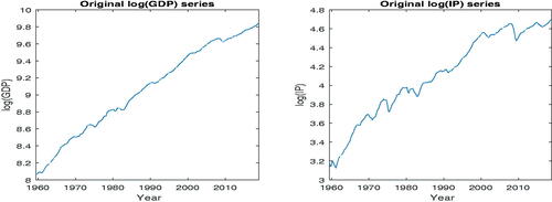
We applied the method in Proposition 1 in Section 2.3.1 to the panel of $N=$ 100 sub-aggregate macroeconomic variables and obtained $\widehat{r}=8,$ where r is the total number of factors and $\widehat{r}$ is as in Proposition 1. Then, we applied the method in Proposition 2 in Section 2.3.1 and obtained $\widehat{p}=4$, where p is the number of I(1) factors. We applied the ADF and the KPSS tests to identify the I(0) and I(1) factors. The validity of using generated factors for ADF and KPSS tests was discussed in Section 2.3.1. Plots of the two high-aggregate macroeconomic variables, GDP and IP, are presented in Figure 1. This figure and the results of ADF test show that these two trended variables are I(1). Further, since we obtained a mixture of I(0) and I(1) factors, the mixture-FAR method developed in this article is well suited for forecasting GDP and IP.

Fig. 1 Time series plots of $\hspace{0.17em}\log \hspace{0.17em}(\mathit{GDP})$ and $\hspace{0.17em}\log \hspace{0.17em}(IP)$ for 1959:Q1 – 2018:Q4.

4.3 Out-of-Sample Forecast Performance of Mixture-FAR Method

4.3.1 The Mixture-FAR and the Basic AR(4) Models

We considered the following four models, the basic AR(4) and three mixture-FAR models obtained by augmenting the AR(4) with a mixture of the I(0) and the I(1) factors: (19) $$\text{Model}\mathrm{ }1\mathrm{ }\text{:}\mathrm{ }{Y}_{t+h}=\alpha \prime {\tilde{E}}_t+\beta \prime {\tilde{G}}_t+\sum _{i=0}^3{\omega }_{1+i}{Y}_{t-i}+{ϵ}_{t+h}\mathrm{\hspace{1em}}\mathrm{\hspace{1em}}$$(19) (20) $$\begin{array}{c}\text{Model}\mathrm{ }2\mathrm{ }\text{:}\mathrm{ }{Y}_{t+h}={\alpha }_1^{\prime }{\tilde{E}}_t+{\alpha }_2^{\prime }{\tilde{E}}_{t-1}+\beta {\prime }_1{\tilde{G}}_t+\beta {\prime }_2{\tilde{G}}_{t-1}\\ +\sum _{i=0}^3{\omega }_{1+i}{Y}_{t-i}+{ϵ}_{t+h}\end{array}$$(20) (21) $$\begin{array}{c}\text{Model}\mathrm{ }3\mathrm{ }\text{:}\mathrm{ }{Y}_{t+h}=\sum _{i=0}^3\alpha {\prime }_{1+i}{\tilde{E}}_{t-i}+\beta {\prime }_1{\tilde{G}}_t\\ +\sum _{i=0}^3{\omega }_{1+i}{Y}_{t-i}+{ϵ}_{t+h}\end{array}$$(21) (22) $$\text{Model}\mathrm{ }4\mathrm{ }\text{:}\mathrm{ }{Y}_{t+h}=\sum _{i=0}^3{\omega }_{1+i}{Y}_{t-i}+{ϵ}_{t+h}.$$(22)

Model 4, the basic AR(4), is used as the benchmark for forecast comparison; since we use quarterly data this is a suitable benchmark. Much of this section focuses on comparing Models 1 to 3 with Model 4, in terms of out-of-sample forecast performance.

4.3.2 Performance of Mixture-FAR Relative to AR(4)

We assess the performance of mixture-FAR models (19)–(21) for forecasting GDP and IP in terms of the out-of-sample R², denoted by $R_{os}^2$, defined in (18). In this section, AR(4) is used as the basic benchmark; later we consider a nonstationary-FAR and a stationary-FAR as the benchmarks. We used the expanding window estimation scheme with three different first estimation periods, and computed the values of $R_{os}^2$ for the three mixture-FAR models (19)–(21) relative to AR(4); they are reported in Table 4. The values of $R_{os}^2$ indicate that the mixture-FAR model, Model 2, outperforms the benchmark model AR(4) for forecasting GDP and IP. Overall, the results presented in Table 4 indicate that Model 2 outperforms the other two models, Models 1 and 3. The results in Table 4 are for expanding windows; for results based on rolling windows, see Section 5.2.1 of the supplementary materials.

4.3.3 Performance of Mixture-FAR Relative to Nonstationary-FAR

For forecasting a nonstationary variable, such as GDP and IP, a nonstationary-FAR model, wherein all the variables including the factors are nonstationary, has been proposed in the literature (Choi 2017). As in the earlier sections, we refer to this model as a nonstationary-FAR model. To implement this method, first we applied principal component analysis to $XX\prime$, chose only the nonstationary factors $\left\{{\tilde{E}}_t\right\}$, and used them as predictors. The nonstationary-FAR model used in this analysis is $$\text{Model\hspace{0.17em}}5[\text{Nonstationary}-\text{FAR}]:$$ $$Y_{t+h}=\beta \prime {\tilde{E}}_t+\sum _{i=0}^3{\omega }_{1+i}{Y}_{t-i}+{ϵ}_{t+h}.$$

We assess the out-of-sample forecast performance of the mixture-FAR model (19) relative to the nonstationary-FAR model Model 5.

The values of $R_{os}^2$ for the mixture-FAR model, Model 1, relative to the nonstationary FAR model, Model 5, are presented in Table 5. The interpretation of the entry 0.31 in the column for $\hspace{0.17em}\log \hspace{0.17em}(IP)$ is the following: For the period 2009–2018, the Sum of Squares of Forecast Error (SSFE) for $\hspace{0.17em}\log \hspace{0.17em}(IP)$ is 31% lower for mixture-FAR compared to the nonstationary-FAR. This table also shows that the SSFE for $\hspace{0.17em}\log \hspace{0.17em}(\mathit{GDP})$ over the period 2009–2018 is 50% lower for mixture-FAR compared to nonstationary-FAR. In fact, Table 5 shows that the mixture-FAR method proposed in this article performed significantly better than the method based on a nonstationary-FAR for forecasting GDP and IP.

4.3.4 Other Observations

Performance of mixture-FAR relative to stationary-FAR

Bai and Ng (2006) proposed a method for forecasting a stationary variable using an FAR model, where all the variables and factors are stationary. We refer to this model/method as a stationary-FAR model/method. We adapt this method for forecasting nonstationary variables. To this end, we use the first differences of GDP and IP; see Section 5.1 in the supplementary materials. The results therein show that the mixture-FAR method performed better than the corresponding stationary-FAR method, for forecasting GDP and IP.

Accounting for possible structural breaks

We extended the empirical study to account for possible structural breaks. The details are presented in Section 5.2 of the supplementary materials. The main observation of these investigations is the following: For dealing with structural breaks/instabilities in our empirical study (a) expanding windows performed better than rolling windows overall, and (b) use of subsamples, with data from a certain period of possible structural break/instabilities removed, did not improve forecasting performance.

4.4 Prediction Intervals

We computed 95% prediction intervals, which are based on the asymptotic results derived in Section 2 and the bootstrap, for one-step-ahead predictions of $\hspace{0.17em}\log \hspace{0.17em}(\mathit{GDP})$ and $\hspace{0.17em}\log \hspace{0.17em}(IP)$. Assuming that the regression error ϵ_t in (2) is normally distributed, we constructed the asymptotic theory-based point-wise 95% prediction intervals for $\hspace{0.17em}\log \hspace{0.17em}(\mathit{GDP})$ and $\hspace{0.17em}\log \hspace{0.17em}(IP)$ for the out-of-sample period 2006:Q1 to 2018:Q4. These intervals are shown in Figure 2 together with the observed values of $\hspace{0.17em}\log \hspace{0.17em}(\mathit{GDP})$ and $\hspace{0.17em}\log \hspace{0.17em}(IP)$.

Fig. 2 Left Panel: One-step ahead point-wise 95% prediction intervals for $\hspace{0.17em}\log \hspace{0.17em}(\mathit{GDP})$ using mixture-FAR. The solid line in the middle is the observed values of $\hspace{0.17em}\log \hspace{0.17em}(\mathit{GDP})$. The pair of dashed lines is the asymptotic theory prediction interval; they are easily identified since one curve appears at the top and the other at the bottom, in 2016. The pair of curves with dash and dot, provide the bootstrap prediction interval. Right Panel: The legend is the same as that for the panel on the left, except that GDP is replaced by IP.

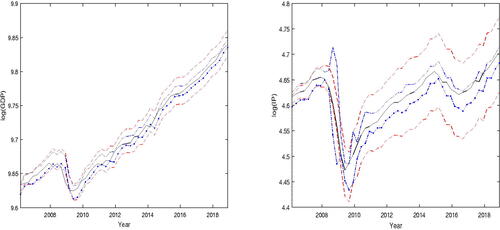
We also estimated the symmetric bootstrap t-percentile prediction intervals using residual bootstrap; to this end, we used 399 bootstrap replications. These are also shown in Figure 2. One important difference between the asymptotic theory-based and bootstrap prediction intervals is that the latter does not assume that the error distribution has a known functional form.

Figure 2 shows that (a) except for a very short interval around the crisis period 2009, the observed values of GDP lie within the two prediction intervals, and (b) every observed value of IP lies within the two prediction intervals. Overall, the bootstrap prediction interval is narrower than the one based on the asymptotic distribution of the forecast, for GDP and IP. The bootstrap prediction interval for IP around the crisis period 2008 is large; this may be because the financial and economic crisis introduced large volatilities in IP around this period. Overall, both prediction intervals have high coverage rates for GDP and IP.

5 Discussion

One topic of interest is the estimation of the numbers of I(0) and I(1) factors in such a way that they are optimal, in some sense, for the purpose of predicting $Y_{T+h}.$ In this article we considered the information criterion method in Bai and Ng (2002) and Bai (2004). In this method, attention is restricted to the factor model only and the objective is to estimate the numbers of factors to explain the variation within $\left\{X_{it}\right\}.$ In some cases, it is possible that all r factors are not needed for forecasting, and fewer than r factors may turn out to have better forecasting performance. This topic has been studied in some recent papers when the FAR model does not have a mixture of I(0) and I(1) factors. In one such approach, residual variance of the factor model, appearing in the information criterion, is replaced by the residual variance from the FAR model (Cheng and Hansen 2015b, Groen and Kapetanios 2013). Another approach is to treat it as a model selection problem with each model being defined by one subset of the factors on the right hand side of the FAR model (Djogbenou 2021). Extensions of these approaches to our setting wherein there is a mixture of I(0) and I(1) factors in the FAR model would be useful.

The proposed methodology can be adjusted for the case when forecasting variable Y_t is stationary. For simplicity, assume that $W_t\sim I(0)$; however, W_t can also be a set of I(1) variables, or a mixture of I(1) and I(0) variables. Let us consider two cases.

• Case 1: Nonstationary factors are assumed to be cointegrated. Let E_t be a vector of I(1) factors, and suppose that they are cointegrated. Let Z_t be a vector of I(0) factors that are linear combinations of E_t. Then, the latent factors, $F_t=(Z_t^{\prime },G_t^{\prime })\prime$, in the model is a set of stationary factors. By Corollary 3 in Bai (2004), we may estimate the dimension of the factors F_t. The estimated factors ${\tilde{F}}_t=({\tilde{Z}}_t^{\prime },{\tilde{G}}_t^{\prime })\prime$ in the model will be a set of stationary processes. We may use this to obtain the forecast of a stationary response variable.

• Case 2: Cointegration of factors is not assumed. In the literature, it has been discussed that a mixture of I(0) and I(1) (also explosive) regressors can be used for forecasting economic and financial time series, see Phillips (2012, 2015). Phillips (2015) considered a basic linear predictive model and obtained the prediction of an I(0) variable using an I(1) time series. Hence, we may use a mixture-FAR model to forecast a stationary Y_t.

An assumption made in this article is that the number of factors r is fixed. It is possible that in some settings it may be appropriate to consider the case when the number of factors in the FAR model increases to $\infty$. With high-dimensional data, such a scenario may well be of interest. The factor model with increasing number of factors is studied in Li, Li, and Shi (2017). An extension to incorporate increasing numbers of I(1) and I(0) factors in the mixture-FAR model is an unexplored area. The extension to our setting with generated I(0) and I(1) factors would require substantial development of new methodology.

When using macroeconomic dataset that spans over a long period of time, instabilities may arise in both factor loadings and parameters of the FAR forecasting model. Stock and Watson (2009) and Banerjee, Marcellino, and Masten (2008) demonstrated that even if the factor loadings are structurally unstable, factors may be estimated consistently if the instability is independent across the panel variables. They recommended the use of rolling window method or time-varying parameters for the estimation of FAR model. Rossi (2021) and Giraitis, Kapetanios, and Price (2013) observed that rolling window was suitable when there are structural instabilities in the dataset. Stock and Watson (2009) and Banerjee, Marcellino, and Masten (2008) have also suggested the use of sub-sample for forecasting when there are such instabilities. We investigated such alternative approaches in our empirical study, and the results are reported in Appendix E.

Recently, among others, Breitung and Eickmeier (2011), Corradi and Swanson (2014), and Su and Wang (2017) developed methods to test and model the instabilities in the factor loadings as well as in the FAR model parameters. Further, Wei and Zhang (2020) considered a time-varying FAR model with time-varying factor loadings to capture the structural breaks in a large panel dataset. They used local PCA to estimate the factor loadings in the factor model and the local constant method to estimate the time-varying coefficients in the forecasting model; the asymptotic validity of this method has not yet been established. To our knowledge, the methodological developments and empirical applications to date covered only the stationary setting: stationary panel data, stationary factors, and forecasting stationary time series. Extensions of these methodological developments to our setting for forecasting a nonstationary variable would be useful.

6 Conclusion

This article developed methodology for forecasting nonstationary macroeconomic variables, such as GDP and IP, when a set of panel data is available for a large number of potential predictors. We propose to estimate a small number of factors using the panel data, and use them as predictors for forecasting. The factors are chosen such that they contain a large proportion of the information in the large number of potential predictors. Typically, such a large number of macroeconomic variables would contain a mixture of stationary and nonstationay variables. Therefore, the factors are also very likely to be a mixture of stationary and nonstationary variables, as illustrated by our empirical example.

This article developed a methodology for using the estimated mixture of stationary and nonstationary factors as predictors, and constructing an asymptotically valid prediction interval. The validity of the coresponding method for forecasting has been established in the literature when all the variables are stationary (Bai and Ng 2006), and also when they are all nonstationary (Choi 2017), but not when they consist of a mixture of stationary and nonstationary variables. Our article contributes to this gap in the literature.

In our simulation study, the mixture-FAR method developed in this article performed better than the one that uses only nonstationary variables. In an empirical study for forecasting GDP and IP, we compared the mixture-FAR method with some competing ones; we observed that the mixture-FAR method performed better. In summary, this article develops an improved method of forecasting a nonstationary variable using information from stationary and nonstationary variables, and it is of practical significance.

Supplementary Materials

The supplementary materials contains the proofs of the theorems stated in Section 2, and some additional results for the sections on the simulation study and the empirical application.

Acknowledgments

We are grateful to the editor, Christian Hansen, an associate editor, and two reviewers for valuable comments and suggestions. We thank Peter Phillips, Sydney Ludvigson, Benjamin Wong, and the participants at the Monash-Xiamen University Workshop and the 40th International Symposium on Forecasting for their comments and suggestions.

Disclosure Statement

The authors report there are no competing interests to declare.

Additional information

Funding

The authors gratefully acknowledge support from the Australian Government through the Australian Research Council’s Discovery Projects funding scheme (projects DP150101012 and DP170104421 for the second author, and project DP150100210 for the third author).

References

- Bai, J. (2003), “Inferential Theory for Factor Models of Large Dimensions,” Econometrica, 71, 135–171. DOI: 10.1111/1468-0262.00392.
- Bai, J. (2004), “Estimating Cross-Section Common Stochastic Trends in Nonstationary Panel Data,” Journal of Econometrics, 122, 137–183.
- Bai, J., and Ng, S. (2002), “Determining the Number of Factors in Approximate Factor Models,” Econometrica, 70, 191–221. DOI: 10.1111/1468-0262.00273.
- Bai, J. (2004), “A Panic Attack on Unit Roots and Cointegration,” Econometrica, 72, 1127–1177.
- Bai, J. (2006), “Confidence Intervals for Diffusion Index Forecasts and Inference for Factor-Augmented Regressions,” Econometrica, 74, 1133–1150.
- Bai, J. (2013), “Principal Components Estimation and Identification of Static Factors,” Journal of Econometrics, 176, 18–29.
- Banerjee, A., Marcellino, M., and Masten, I. (2008), “Forecasting Macroeconomic Variables Using Diffusion Indexes in Short Samples with Structural Change,” in Forecasting in the Presence of Structural Breaks and Model Uncertainty (Frontiers of Economics and Globalization) (Vol. 3), eds. D. Rapach and M. Wohar, pp. 149–194, Bingley, UK: Emerald Group Publishing Limited.
- Bernanke, B. S., Boivin, J., and Eliasz, P. (2005), “Measuring the Effects of Monetary Policy: A Factor-Augmented Vector Autoregressive (favar) Approach,” The Quarterly Journal of Economics, 120, 387–422. DOI: 10.1162/qjec.2005.120.1.387.
- Breitung, J., and Eickmeier, S. (2011), “Testing for Structural Breaks in Dynamic Factor Models,” Journal of Econometrics, 163, 71–84. DOI: 10.1016/j.jeconom.2010.11.008.
- Cheng, X., and Hansen, B. E. (2015a), “Forecasting with Factor-Augmented Regression: A Frequentist Model Averaging Approach,” Journal of Econometrics, 186, 280–293. DOI: 10.1016/j.jeconom.2015.02.010.
- Cheng, X. (2015b), “Forecasting with Factor-Augmented Regression: A Frequentist Model Averaging Approach,” Journal of Econometrics, 186, 280–293.
- Choi, I. (2017), “Efficient Estimation of Nonstationary Factor Models,” Journal of Statistical Planning and Inference, 183, 18–43. DOI: 10.1016/j.jspi.2016.10.003.
- Corradi, V., and Swanson, N. R. (2014), “Testing for Structural Stability of Factor Augmented Forecasting Models,” Journal of Econometrics, 182, 100–118. DOI: 10.1016/j.jeconom.2014.04.011.
- Djogbenou, A. A. (2021), “Model Selection in Factor-Augmented Regressions with Estimated Factors,” Econometric Reviews, 40, 470–503. DOI: 10.1080/07474938.2020.1808371.
- Eickmeier, S. (2005), “Common Stationary and Non-stationary Factors in the Euro Area Analyzed in a Large-Scale Factor Model,” Discussion paper 2, Studies of the Economic Research Centre.
- Giraitis, L., Kapetanios, G., and Price, S. (2013), “Adaptive Forecasting in the Presence of Recent and Ongoing Structural Change,” Journal of Econometrics, 177, 153–170. DOI: 10.1016/j.jeconom.2013.04.003.
- Gonçalves, S., and Perron, B. (2014), “Bootstrapping Factor-Augmented Regression Models,” Journal of Econometrics, 182, 156–173. DOI: 10.1016/j.jeconom.2014.04.015.
- Groen, J. J. J., and Kapetanios, G. (2013), “Model Selection Criteria for Factor-Augmented Regressions,” Oxford Bulletin of Economics and Statistics, 75, 37–63. DOI: 10.1111/j.1468-0084.2012.00721.x.
- Li, H., Li, Q., and Shi, Y. (2017), “Determining the Number of Factors when the Number of Factors can Increase with Sample Size,” Journal of Econometrics, 197, 76–86. DOI: 10.1016/j.jeconom.2016.06.003.
- Ludvigson, S. C., and Ng, S. (2007), “The Empirical Risk–Return Relation: A Factor Analysis Approach,” Journal of Financial Economics, 83, 171–222. DOI: 10.1016/j.jfineco.2005.12.002.
- Moon, H. R., and Perron, B. (2007), “An Empirical Analysis of Nonstationarity in a Panel of Interest Rates with Factors,” Journal of Applied Econometrics, 22, 383–400. DOI: 10.1002/jae.931.
- Phillips, P. C. (2012), “Folklore Theorems, Implicit Maps, and Indirect Inference,” Econometrica, 80, 425–454.
- Phillips, P. C. (2015), “Halbert White jr. Memorial JFEC Lecture: Pitfalls and Possibilities in Predictive Regression,” Journal of Financial Econometrics, 13, 521–555.
- Rossi, B. (2021), “Forecasting in the Presence of Instabilities: How We Know Whether Models Predict Well and How to Improve Them,” Journal of Economic Literature, 59, 1135–90. DOI: 10.1257/jel.20201479.
- Smeekes, S., and Wijler, E. (2019), “High-Dimensional Forecasting in the Presence of Unit Roots and Cointegration,” Working paper, Department of Quantitative Economics, Maastricht University.
- Stock, J. H., and Watson, M. W. (1998a), “A Comparison of Linear and Nonlinear Univariate Models for Forecasting Macroeconomic Time Series,” Technical Report, National Bureau of Economic Research.
- Stock, J. H. (1998b), “Diffusion Indexes,” Technical Report, National Bureau of Economic Research.
- Stock, J. H. (2002a), “Forecasting Using Principal Components from a Large Number of Predictors,” Journal of the American Statistical Association, 97, 1167–1179.
- Stock, J. H. (2002b), “Macroeconomic Forecasting Using Diffusion Indexes,” Journal of Business & Economic Statistics, 20, 147–162.
- Stock, J. H. (2009), “Forecasting in Dynamic Factor Models Subject to Structural Instability,” in The Methodology and Practice of Econometrics. A Festschrift in Honour of David F. Hendry (Vol. 173), eds. N. Shephard and J. Castle, p. 205, Oxford: Oxford University Press.
- Stock, J. H. (2012), “Generalized Shrinkage Methods for Forecasting Using Many Predictors,” Journal of Business & Economic Statistics, 30, 481–493.
- Su, L., and Wang, X. (2017), “On Time-Varying Factor Models: Estimation and Testing,” Journal of Econometrics, 198, 84–101. DOI: 10.1016/j.jeconom.2016.12.004.
- Wei, J., and Zhang, Y. (2020), “A Time-Varying Diffusion Index Forecasting Model,” Economics Letters, 193, 109337. DOI: 10.1016/j.econlet.2020.109337.