Two-Sample Testing for Tail Copulas with an Application to Equity Indices

Abstract

A novel, general two-sample hypothesis testing procedure is established for testing the equality of tail copulas associated with bivariate data. More precisely, using a martingale transformation of a natural two-sample tail copula process, a test process is constructed, which is shown to converge in distribution to a standard Wiener process. Hence, from this test process a myriad of asymptotically distribution-free two-sample tests can be obtained. The good finite-sample behavior of our procedure is demonstrated through Monte Carlo simulations. Using the new testing procedure, no evidence of a difference in the respective tail copulas is found for pairs of negative daily log-returns of equity indices during and after the global financial crisis.

Keywords:

• Distribution-free testing
• Financial crisis
• Martingale transformation
• Tail copula
• Tail dependence
• Two-sample testing

1 Introduction

Measuring dependence between economic variables such as asset returns and, in particular, between their tail events is of crucial importance for risk management, asset pricing, and portfolio choice. The tail dependence structure is, for example, a main ingredient for the computation of high quantiles of aggregate loss distributions, and hence for risk capital requirements, and dictates the extent of idiosyncratic tail risk, and hence the diversification potential, within a collection of assets.

A key question in financial econometrics and international finance is whether the dependence structure between economic variables, in particular asset returns, is constant over time and across markets, regions and institutions, or whether it is subject to variation due to for example, financial market integration, emerging market developments, or financial contagion. Several papers analyze this question using a wide variety of different methodologies; see for example, King and Wadhwani (1990), Longin and Solnik (1995), Forbes and Rigobon (2002), Bekaert, Harvey, and Ng (2005), Bekaert, Hodrick, and Zhang (2009), Christoffersen et al. (2012), Bücher, Jäschke, and Wied (2015), Bormann and Schienle (2020), and the references therein.

In this article, we focus on the tail dependence structure between two risks, which is completely characterized by the bivariate tail copula. In this context, we develop a general procedure to test for the equality of the tail copulas associated with two bivariate samples. The standard one-sample problem, that is, testing for a specific parametric family of tail copulas, has been studied in Can et al. (2015). A challenging feature of the two-sample problem is that the—under the null hypothesis—common tail copula is not specified. This complexity arises naturally as it follows from de Haan and Resnick (1977) that the class of all possible tail copulas is so large that it cannot be represented as a finite-dimensional parametric family, rendering the testing problem nonparametric. A pivotal property of our procedure is that, through a martingale transformation, it leads to asymptotically distribution-free test statistics, so that critical values can be tabulated for universal use and no computer-intensive methods have to be developed and validated.

Our testing approach can be summarized as follows. We first construct two semi-parametric estimators of the tail copulas, one for each sample, consider their suitably normalized difference, and prove that it converges weakly to a nontrivial limiting process under the null hypothesis of tail copula equality. Next, we describe the martingale transformation that transforms this limiting process into a standard bivariate Wiener process. Then, we establish that the empirical counterpart of this transformation, when applied to the empirical process given by the normalized difference of the two tail copula estimators, converges weakly to a standard bivariate Wiener process under the null hypothesis. Finally, two-sample tests for tail copulas can now be conducted by comparing the transformed empirical process to a standard Wiener process. Hence, our approach leads to an asymptotically distribution-free test process and thus, by taking functionals, to asymptotically distribution-free test statistics. In other words, our procedure leads to an entire test process from which we can generate a myriad of asymptotically distribution-free tests.

We illustrate the finite-sample performance of our approach through Monte Carlo simulations. These confirm that tests based on our test process have good size and power performances, notwithstanding the difficult nature of the testing problem considered in this article.

We apply our procedure to test for tail copula equality of equity index returns during and after the global financial crisis. In particular, we analyze the tail dependence structure among the two European equity market indices FTSE 100 (UK) and DAX 30 (Germany) and the two transatlantic equity indices FTSE 100 and S&P 500 (US), during 2008–2011 (sample 1, covering the most volatile days of the global financial crisis and the subsequent European debt crisis) and 2012–2015 (sample 2, covering a “post-crisis” period of equal length). We construct synchronized daily observations of negative log-returns on the basis of high-frequency data using Coordinated Universal Time (UTC). Computing three commonly used test statistics from our test process, we find that the null hypothesis of tail copula equality between the two samples is not rejected, despite a clearly visible change in the marginal distributions of the index returns between the two samples. This finding applies to both the European pair {FTSE 100, DAX 30} and the transatlantic pair {FTSE 100, S&P 500}. That is, although the margins became markedly less volatile from the crisis period to the post-crisis period, no statistical evidence is found for a change in the number of margin-free joint extremes for both pairs of equity market indices.

We briefly describe four papers that are related to the testing problem considered in this article. In Christoffersen et al. (2012), an extensive analysis is conducted of the evolution over time of the regular and tail dependence structures among both developed and emerging financial markets, and the associated diversification potential. Econometrically, a novel dynamic asymmetric copula model of a parametric nature is used to capture asymmetric tail dependence. When assessing tail dependence, attention is restricted to the less informative tail dependence coefficients, rather than to tail copula functions as in the present paper, and their development over a long period of 20 years. In Bücher and Dette (2013) and Bücher, Jäschke, and Wied (2015), new statistical methods are developed for testing tail copula equality, tail copula goodness-of-fit testing, and detecting structural breaks in tail dependence. The methods are applied in Bücher, Jäschke, and Wied (2015) to energy and financial markets data. An important difference between these two papers and the present one is that here convenient distribution-free weak limits of test statistics are obtained, as described above, whereas in Bücher and Dette (2013) and Bücher, Jäschke, and Wied (2015) computer-intensive multiplier bootstrap procedures are employed. Bormann and Schienle (2020) provides a detailed account of tail dependence asymmetries and inequalities in 90 years of U.S. equity data, using a refined nonparametric testing procedure that compares two tail copulas locally piecewise on disjoint intervals employing multiple testing principles. As the corresponding complex limiting distributions do not admit closed-form expressions, finite-sample approximations are simulated using multiplier bootstrap procedures, as in Bücher and Dette (2013) and Bücher, Jäschke, and Wied (2015).

The remainder of this article is organized as follows. In Section 2 we formalize our testing problem and in Section 3 we introduce our initial testing basis, which compares two semi-parametric tail copula estimators constructed separately from the two samples, and analyze its asymptotic behavior. In Section 4 we describe the martingale transformation and in Section 5 we prove that the empirical counterpart of this transformation applied to our initial testing basis converges weakly to a standard Wiener process. In Section 6 our Monte Carlo simulation analysis is presented. Section 7 describes the results of our empirical analysis of equity indices. Conclusions are given in Section 8. The proofs of our theorems and some additional simulation results are deferred to the Appendix, supplementary materials. An R script implementing our testing approach is also provided as a supplementary material.

2 Testing Problem

Consider iid random vectors $(X_1,Y_1),\dots ,(X_n,Y_n)$ generated from some bivariate distribution function (df) F and iid random vectors $(X{\prime }_1,Y{\prime }_1),$ $\dots ,(X{\prime }_n,Y{\prime }_n)$ independently generated from some bivariate df $F\prime$. Let F have marginal dfs F₁, F₂ and let $F\prime$ have marginal dfs $F{\prime }_1,F{\prime }_2$, so that $X_i\sim F_1,Y_i\sim F_2$ and $X{\prime }_i\sim F{\prime }_1,Y{\prime }_i\sim F{\prime }_2$ for $i=1,\dots ,n$.

We assume that the dfs F and $F\prime$ lie in the respective domains of attraction of bivariate extreme value distributions G and $G\prime$. This means that there exist normalizing sequences $a_j(n),a{\prime }_j(n)>0$ and $b_j(n),b{\prime }_j(n)\in \mathbb{R}$, for j = 1, 2, such that$$\begin{array}{c}P(\frac{{⏧}_{i=1}^n{X}_i-b_1(n)}{a_1(n)}\le x,\frac{{⏧}_{i=1}^n{Y}_i-b_2(n)}{a_2(n)}\le y)\to G(x,y),\\ P(\frac{{⏧}_{i=1}^{n}X{\prime }_i-b{\prime }_1(n)}{a{\prime }_1(n)}\le x,\frac{{⏧}_{i=1}^{n}Y{\prime }_i-b{\prime }_2(n)}{a{\prime }_2(n)}\le y)\to G\prime (x,y),\end{array}$$as $n\to \infty$, for all continuity points $(x,y)\in {\mathbb{R}}^2$ of G and $G\prime$, respectively. The normalizing sequences are chosen in such a way that the margins G₁, G₂, of G, and the margins $G{\prime }_1,G{\prime }_2$, of $G\prime$, are in the form of a standard generalized extreme value (GEV) distribution:(1) $$\begin{array}{cc}{G}_j(x)\hfill & =\hspace{0.17em}\exp \hspace{0.17em}\{-{(1+{\gamma }_{j}x)}^{-1/{\gamma }_j}\},\hspace{1em}1+{\gamma }_{j}x>0,\hfill \\ G{\prime }_j(x)\hfill & =\hspace{0.17em}\exp \hspace{0.17em}\{-{(1+\gamma {\prime }_{j}x)}^{-1/\gamma {\prime }_j}\},\hspace{1em}1+\gamma {\prime }_{j}x>0,\hfill \end{array}$$(1) for j = 1, 2. The constants ${\gamma }_1,{\gamma }_2\in \mathbb{R}$ and $\gamma {\prime }_1,\gamma {\prime }_2\in \mathbb{R}$ are the marginal extreme value (EV) indices associated with F and $F\prime$, respectively. Here, and in the rest of the article, expressions of the form ${(1+\gamma · )}^{1/\gamma }$ should be interpreted as $\hspace{0.17em}\exp \hspace{0.17em}(·)$ when γ = 0.

The distribution G, hence, the asymptotic joint tail behavior of F, is characterized by the marginal EV indices ${\gamma }_1,{\gamma }_2$ and the bivariate tail copula R associated with F, which can be defined as(2) $$\begin{array}{cc}R(x,y)\hfill & :=\underset{t\to \infty }{\lim }tP(F_1(X_1)>1-x/t,F_2(Y_1)>1-y/t),\hfill \\ \hfill & (x,y)\in {[0,\infty ]}^2\setminus \{(\infty ,\infty )\}.\hfill \end{array}$$(2)

The EV indices ${\gamma }_1,{\gamma }_2$ specify the margins of G through (1), and the function R specifies the dependence structure between the margins. While R is not a copula itself, it does characterize the copula of G, and hence the tail dependence structure of F. Similarly, the distribution $G\prime$ is characterized by $\gamma {\prime }_1,\gamma {\prime }_2$ and the tail copula $R\prime$ associated with $F\prime$, defined analogously to (2). We refer to, for example, the monographs Kotz and Nadarajah (2000), Beirlant et al. (2004), and de Haan and Ferreira (2006) for further details about multivariate extreme value theory.

Observe that$$R(1,1)=\underset{u\uparrow 1}{\lim }\frac{P(F_1(X_1)>u,F_2(Y_1)>u)}{1-u}.$$

For random variables with continuous margins, R(1, 1) is often referred to as the upper tail dependence coefficient and denoted by λ_U; see for example, Joe (2001), p. 33. It measures the probability of a “large rank” of X₁ conditionally upon a “large rank” of Y₁. Indeed,$${\lambda }_U=\underset{u\uparrow 1}{\lim }P(F_1(X_1)>u|F_2(Y_1)>u)=R(1,1).$$

We also note here that the function R generates a σ-finite measure R on the Borel subsets of ${[0,\infty ]}^2\setminus \{(\infty ,\infty )\}$ via the identity$$R([0,x]\times [0,y]):=R(x,y),\hspace{1em}(x,y)\in {[0,\infty ]}^2\setminus \{(\infty ,\infty )\}.$$

In this article, we develop a general procedure to construct two-sample tests for the equality of the tail copulas R and $R\prime$. In other words, we assume that we have two random samples independently generated from F and $F\prime$, and provide a procedure that can be used to test the null hypothesis $R=R\prime$ against the alternative $R\ne R\prime$, where R and $R\prime$ remain unspecified. Note that, while the bivariate extreme value setting is of a semi-parametric nature, both the null and alternative hypotheses we consider in this article are nonparametric.

3 Comparing Two Tail Copula Estimators

Suppose we have a random sample $(X_1,Y_1),\dots ,(X_n,Y_n)$ from F and an independent random sample $(X{\prime }_1,Y{\prime }_1),\dots ,(X{\prime }_{n\prime },Y{\prime }_{n\prime })$ from $(X_1,Y_1),\dots ,(X_n,Y_n)$. Throughout Sections 3–5 we will assume that the null hypothesis holds, that is, R and $R\prime$ are the same tail copula, which we will refer to as R. In the present section, we define two semi-parametric estimators for the tail copula R, computed separately from the two available samples, and we describe the asymptotic behavior of the difference between these two estimators as the sample sizes tend to infinity.

From (2), one can verify that $R(x,y)=\underset{t\to \infty }{\lim }{R}_{(t)}(x,y)$ for $(x,y)\in {[0,\infty )}^2$, with(3) $$R_{(t)}(x,y)=tP({\tilde{X}}_1(t)\le x,{\tilde{Y}}_1(t)\le y),\hspace{1em}(x,y)\in {[0,\infty )}^2,$$(3) where(4) $$\begin{array}{cc}{\tilde{X}}_i(t)\hfill & ={[(1+{\gamma }_1\frac{X_i-b_1(t)}{a_1(t)})\vee 0]}^{-1/{\gamma }_1},\hspace{1em}1\le i\le n,\hfill \\ {\tilde{Y}}_i(t)\hfill & ={[(1+{\gamma }_2\frac{Y_i-b_2(t)}{a_2(t)})\vee 0]}^{-1/{\gamma }_2},\hspace{1em}1\le i\le n.\hfill \end{array}$$(4)

We also define $\tilde{X}{\prime }_i(t),\tilde{Y}{\prime }_i(t)$ analogously to (4) and $R{\prime }_{(t)}$ analogously to (3). We will use the functions $R_{(t)}$ and $R{\prime }_{(t)}$ as a basis for estimating R from the two available samples. To that end, we let $k=k(n)$ and $k\prime =k\prime (n\prime )$ denote intermediate sequences satisfying $k\uparrow \infty ,k/n\downarrow 0$ as $n\uparrow \infty$ and $k\prime \uparrow \infty ,k\prime /n\prime \downarrow 0$ as $n\prime \uparrow \infty$. For notational brevity, we will write R_n for $R_{(n/k)}$ and $R{\prime }_{n\prime }$ for $R{\prime }_{(n\prime /k\prime )}$.

We estimate R_n and hence R by replacing the unknown quantities $a_j(n/k),b_j(n/k)$ and γ_j in (4) by appropriate estimators ${\widehat{a}}_j(n/k),{\widehat{b}}_j(n/k)$ and ${\widehat{\gamma }}_j$, for j = 1, 2, and the probability P by the corresponding empirical measure. We define, therefore,(5) $$\begin{array}{cc}{\widehat{X}}_i(n/k)\hfill & ={[(1+{\widehat{\gamma }}_1\frac{X_i-{\widehat{b}}_1(n/k)}{{\widehat{a}}_1(n/k)})\vee 0]}^{-1/{\widehat{\gamma }}_1},\hspace{1em}1\le i\le n,\hfill \\ {\widehat{Y}}_i(n/k)\hfill & ={[(1+{\widehat{\gamma }}_1\frac{Y_i-{\widehat{b}}_2(n/k)}{{\widehat{a}}_2(n/k)})\vee 0]}^{-1/{\widehat{\gamma }}_2},\hspace{1em}1\le i\le n,\hfill \end{array}$$(5) as an empirical analogue to (4), and we introduce the semi-parametric estimator(6) $${\widehat{R}}_n(x,y)=\frac{1}{k}\sum _{i=1}^n\mathrm{ }{1}_{\{{\widehat{X}}_i(n/k)\le x,{\widehat{Y}}_i(n/k)\le y\}},\hspace{1em}(x,y)\in {[0,\infty )}^2,$$(6) for the tail copula R. The random variables $\widehat{X}{\prime }_i(n\prime /k\prime ),\widehat{Y}{\prime }_i(n\prime /k\prime )$ and the estimator $\widehat{R}{\prime }_{n\prime }(x,y)$ are defined analogously to (5) and (6), respectively.

Throughout, we fix δ and T such that $0<\delta <T<\infty$. For later reference, we also introduce the process(7) $$T_n(x,y)=\frac{1}{k}\sum _{i=1}^n\mathrm{ }{1}_{\{{\tilde{X}}_i(n/k)\le x,{\tilde{Y}}_i(n/k)\le y\}},\hspace{1em}(x,y)\in {[0,\infty )}^2,$$(7) and the analogously defined $T{\prime }_{n\prime }$. It is known, by (Einmahl, de Haan, and Sinha 1997, Lemma 3.1), that the weak convergence$$(\sqrt{k}(T_n-R_n),\sqrt{k\prime }(T{\prime }_{n\prime }-R{\prime }_{n\prime }))\Rightarrow (V_R,V{\prime }_R)$$ holds in the product space $D({[\delta /2,T+1]}^2)\times D({[\delta /2,T+1]}^2)$ as $n,n\prime \to \infty$. Here, $D({[\delta /2,T+1]}^2)$ denotes the Skorokhod space of functions with domain ${[\delta /2,T+1]}^2$, and $V_R,V{\prime }_R$ are independent R-Wiener processes on ${[0,\infty )}^2$, that is, independent zero-mean Gaussian processes with covariance structure$$E[V_R(s,t)V_R(x,y)]=E[V{\prime }_R(s,t)V{\prime }_R(x,y)]=R(s\wedge x,t\wedge y).$$

Henceforth, we will omit the arguments $(n/k)$ and $(n\prime /k\prime )$ where appropriate, for ease of notation.

Now, the estimators ${\widehat{R}}_n$ and $\widehat{R}{\prime }_{n\prime }$ estimate the same tail copula R from two different samples, while they would estimate different tail copulas under the alternative hypothesis. So the normalized difference between ${\widehat{R}}_n$ and $\widehat{R}{\prime }_{n\prime }$ is a natural starting point for a two-sample test. Thus, we define $\kappa :=kk\prime /(k+k\prime )$ and$${\eta }_{n,n\prime }(x,y):=\sqrt{\kappa }[{\widehat{R}}_n(x,y)-\widehat{R}{\prime }_{n\prime }(x,y)],\hspace{1em}(x,y)\in {[0,\infty )}^2.$$

Our first result will establish the asymptotic behavior of ${\eta }_{n,n\prime }$ as $n,n\prime \to \infty$. We first state the necessary assumptions and definitions.

A1. For some 6-variate random vector $(A_1,A_2,B_1,B_2,{\Gamma }_1,{\Gamma }_2)$, we have the joint weak convergence(8) $$\begin{array}{c}\sqrt{k}(T_n-R_n,\frac{{\widehat{a}}_1}{a_1}-1,\frac{{\widehat{a}}_2}{a_2}-1,\frac{{\widehat{b}}_1-b_1}{a_1},\frac{{\widehat{b}}_2-b_2}{a_2},{\widehat{\gamma }}_1-{\gamma }_1,{\widehat{\gamma }}_2-{\gamma }_2)\\ \mathrm{\hspace{1em}}\mathrm{\hspace{1em}}\Rightarrow (V_R,A_1,A_2,B_1,B_2,{\Gamma }_1,{\Gamma }_2)\end{array}$$(8) as $n\to \infty$, in $D({[\delta /2,T+1]}^2)\times {\mathbb{R}}^6$. Similarly, for some 6-variate random vector $(A{\prime }_1,A{\prime }_2,$ $B{\prime }_1,B{\prime }_2,\Gamma {\prime }_1,\Gamma {\prime }_2)$, we have the joint weak convergence(9) $$\begin{array}{c}\sqrt{k\prime }(T{\prime }_{n\prime }-R{\prime }_{n\prime },\frac{\widehat{a}{\prime }_1}{a{\prime }_1}-1,\frac{\widehat{a}{\prime }_2}{a{\prime }_2}-1,\frac{\widehat{b}{\prime }_1-b{\prime }_1}{a{\prime }_1},\frac{\widehat{b}{\prime }_2-b{\prime }_2}{a{\prime }_2},\widehat{\gamma }{\prime }_1-\gamma {\prime }_1,\widehat{\gamma }{\prime }_2-\gamma {\prime }_2)\\ \mathrm{\hspace{1em}}\mathrm{\hspace{1em}}\Rightarrow (V{\prime }_R,A{\prime }_1,A{\prime }_2,B{\prime }_1,B{\prime }_2,\Gamma {\prime }_1,\Gamma {\prime }_2)\end{array}$$(9) as $n\prime \to \infty$, in $D({[\delta /2,T+1]}^2)\times {\mathbb{R}}^6$.

Assumption A1 is formulated such that it allows for flexibility in choosing the estimators. It is fulfilled for, for example, the moment estimators of γ_j, a_j, b_j, $\gamma {\prime }_j,a{\prime }_j$, and $b{\prime }_j$, provided that k and $k\prime$ are chosen appropriately; see de Haan and Ferreira (2006), sec. 4.2 and 3.5.

A2. The partial derivatives $R^{(1)}(x,y):=\partial R/\partial x$ and $R^{(2)}(x,y):=\partial R/\partial y$ exist and are continuous on ${(0,\infty )}^2$.

A3. (i) For some $\varphi ,\varphi \prime >0$, as $t\to \infty$,$$\begin{array}{c}\underset{(x,y)\in {[\delta /2,T+1]}^2}{\sup }|R_{(t)}(x,y)-R(x,y)|=O(t^{-\varphi }),\\ \underset{(x,y)\in {[\delta /2,T+1]}^2}{\sup }|R{\prime }_{(t)}(x,y)-R(x,y)|=O(t^{-\varphi \prime }).\end{array}$$

(ii) The sequences k and $k\prime$ satisfy$$k=o(n^{2\varphi /(2\varphi +1)})\mathrm{ }\text{as}\mathrm{ }n\to \infty ,\hspace{1em}k\prime =o({(n\prime )}^{2\varphi \prime /(2\varphi \prime +1)})\mathrm{ }\text{as}\mathrm{ }n\prime \to \infty ,$$and $k\prime /(k+k\prime )\to c$ for some $c\in (0,1)$ as $n,n\prime \to \infty$.

Finally, for x > 0 and $\gamma \in \mathbb{R}$, we define the following functions:(10) $$\begin{array}{cc}f(x,\gamma )=\{\begin{array}{cc}\frac{x(x^{\gamma }-1)}{\gamma }\hfill & \gamma \ne 0\hfill \\ x\hspace{0.17em}\log \hspace{0.17em}x\hfill & \gamma =0\hfill \end{array},g(x,\gamma )\hfill & =-x^{\gamma +1},\hfill \\ h(x,\gamma )=\{\begin{array}{cc}\frac{x(1-x^{\gamma })}{{\gamma }^2}+\frac{x\hspace{0.17em}\log \hspace{0.17em}x}{\gamma }\hfill & \gamma \ne 0\hfill \\ -(x{\hspace{0.17em}\log \hspace{0.17em}}^{2}x)/2\hfill & \gamma =0\hfill \end{array}.\hfill & \hfill \end{array}$$(10)

We are now prepared to state the convergence result for ${\eta }_{n,n\prime }$.

Theorem 3.1.

If Assumptions A1–A3 hold, then(11) $$\begin{array}{c}{\eta }_{n,n\prime }(x,y)\Rightarrow \sqrt{c} V_R(x,y)-\sqrt{1-c} V{\prime }_R(x,y)\\ +\sqrt{c} R^{(1)}(x,y)[f(x,{\gamma }_1)A_1\\ +g(x,{\gamma }_1)B_1+h(x,{\gamma }_1){\Gamma }_1]\\ +\sqrt{c} R^{(2)}(x,y)[f(y,{\gamma }_2)A_2\\ +g(y,{\gamma }_2)B_2+h(y,{\gamma }_2){\Gamma }_2]\\ -\sqrt{1-c} R^{(1)}(x,y)[f(x,\gamma {\prime }_1)A{\prime }_1\\ +g(x,\gamma {\prime }_1)B{\prime }_1+h(x,\gamma {\prime }_1)\Gamma {\prime }_1]\\ -\sqrt{1-c} R^{(2)}(x,y)[f(y,\gamma {\prime }_2)A{\prime }_2\\ +g(y,\gamma {\prime }_2)B{\prime }_2+h(y,\gamma {\prime }_2)\Gamma {\prime }_2]\\ =:\eta (x,y)\end{array}$$(11) in $D({[\delta ,T]}^2)$ as $n,n\prime \to \infty$.

Remark 3.2.

While the normalized difference between ${\widehat{R}}_n$ and $\widehat{R}{\prime }_{n\prime }$ provides a natural initial basis for two-sample testing, Theorem 3.1 reveals that it is not easily amenable for this purpose: the distribution of η depends upon the true underlying tail copula R, which is not specified by the null hypothesis, as well as on the true, but unknown, values of the parameters γ₁, γ₂, $\gamma {\prime }_1$ and $\gamma {\prime }_2$. To obtain a suitable testing basis, we will in the next section describe a martingale transformation that will turn η into a standard process with a distribution that depends neither on R nor on the marginal extreme value indices.

Remark 3.3.

The following relationships between the functions f, g, h defined in (10) can be verified, for any x > 0 and $\gamma ,\gamma \prime \in \mathbb{R}$:$$\begin{array}{c}\gamma f(x,\gamma )+g(x,\gamma )=\gamma \prime f(x,\gamma \prime )+g(x,\gamma \prime ),\\ \gamma h(x,\gamma )+f(x,\gamma )=\gamma \prime h(x,\gamma \prime )+f(x,\gamma \prime ).\end{array}$$

Using these identities, the limiting process η appearing in (11) can also be written as$$\begin{array}{c}\eta (x,y)=\sqrt{c} V_R(x,y)-\sqrt{1-c} V{\prime }_R(x,y)\\ +R^{(1)}(x,y)[f(x,{\gamma }_1)(\sqrt{c} A_1+\sqrt{1-c} A{\prime }_1\\ +({\gamma }_1-\gamma {\prime }_1)\sqrt{1-c} B{\prime }_1)\\ +g(x,{\gamma }_1)(\sqrt{c} B_1+\sqrt{1-c} B{\prime }_1)\\ +h(x,{\gamma }_1)(\sqrt{c} {\Gamma }_1+{\gamma }_1\sqrt{1-c} A{\prime }_1-{\gamma }_1\gamma {\prime }_1\sqrt{1-c} B{\prime }_1)\\ -h(x,\gamma {\prime }_1) (\sqrt{1-c} \Gamma {\prime }_1-\gamma {\prime }_1\sqrt{1-c} A{\prime }_1+{(\gamma {\prime }_1)}^2\sqrt{1-c} B{\prime }_1)]\\ +R^{(2)}(x,y)[f(y,{\gamma }_2)(\sqrt{c} A_2+\sqrt{1-c} A{\prime }_2\\ +({\gamma }_2-\gamma {\prime }_2)\sqrt{1-c} B{\prime }_2)+g(y,{\gamma }_2)(\sqrt{c} B_2+\sqrt{1-c} B{\prime }_2)\\ +h(y,{\gamma }_2)(\sqrt{c} {\Gamma }_2+{\gamma }_1\sqrt{1-c} A{\prime }_2-{\gamma }_2\gamma {\prime }_2\sqrt{1-c} B{\prime }_2)\\ -h(y,\gamma {\prime }_2) (\sqrt{1-c} \Gamma {\prime }_2-\gamma {\prime }_2\sqrt{1-c} A{\prime }_2+{(\gamma {\prime }_2)}^2\sqrt{1-c} B{\prime }_2)].\end{array}$$

This equivalent, but—importantly—more parsimonious, form of the limiting process η, rather than that in (11), will serve as the basis for the martingale transformation described in the next section, which would otherwise be ill-defined.

Remark 3.4.

Although the bivariate case is the most interesting and the most relevant one, the setup and results of this article can be generalized to the d-variate case, for d > 2. We will not pursue this, however, because for d > 2 a d-variate tail copula R on the domain ${[0,\infty )}^d$ yields, in contrast to when d = 2, only limited information on the tail dependence structure of F.

4 Martingale Transformation

In this section, we describe a martingale transformation that enables us to transform the limiting process η into a standard bivariate Wiener process. The transformation is obtained by a suitable application of the martingale innovation transform approach originally developed in Khmaladze (1981, 1988, 1993), and used for example, in Koenker and Xiao (2002, 2006) for quantile regression, in Khmaladze and Koul (2004) and Delgado, Hidalgo, and Velasco (2005) for goodness-of-fit testing of parametric regression and time series models, and used and extended in Can et al. (2015) for parametric tail copula goodness-of-fit testing. The classical Doob-Meyer decomposition of a Brownian bridge, which turns a Brownian bridge into a standard Brownian motion by subtracting its compensator, occurs as a simple special case of this approach. Heuristically, the present martingale transformation may therefore be understood as the suitable counterpart for η of the Doob-Meyer decomposition for a Brownian bridge.

Consider the representation we derived in Remark 3.3 for the limiting process η of Theorem 3.1. It is easy to see, by direct computation of the covariance, that the process $\sqrt{c} V_R(x,y)-\sqrt{1-c} V{\prime }_R(x,y)$ is an R-Wiener process, which we will call ${\tilde{V}}_R$. Thus, η is of the form(12) $$\eta (x,y)={\tilde{V}}_R(x,y)+\sum _{i=1}^8{Q}_i(x,y)Z_i,\hspace{1em}(x,y)\in {(0,\infty )}^2,$$(12) where the Z_i are random variables and the Q_i are deterministic functions on ${(0,\infty )}^2$, defined by(13) $$\begin{array}{c}{Q}_1(x,y)=R^{(1)}(x,y) f(x,{\gamma }_1),Q_2(x,y)=R^{(2)}(x,y) f(y,{\gamma }_2),\\ Q_3(x,y)=R^{(1)}(x,y) g(x,{\gamma }_1),Q_4(x,y)=R^{(2)}(x,y) g(y,{\gamma }_2),\\ Q_5(x,y)=R^{(1)}(x,y) h(x,{\gamma }_1),Q_6(x,y)=R^{(2)}(x,y) h(y,{\gamma }_2),\\ Q_7(x,y)=R^{(1)}(x,y) h(x,\gamma {\prime }_1),Q_8(x,y)=R^{(2)}(x,y) h(y,\gamma {\prime }_2).\end{array}$$(13)

We note that (12) is of the general bivariate form (23) in Can et al. (2015). Hence, η can be transformed into a standard Wiener process by suitably exploiting Theorem 3.1 of that paper. We will formally state this result in Theorem 4.1, but we first introduce some assumptions and notation.

A4. The tail copula R has a positive density $r={\partial }^{2}R/\partial x\partial y$ on ${(0,\infty )}^2$. The derivatives $r^{(1)}:=\partial r/\partial x$ and $r^{(2)}:=\partial r/\partial y$ exist and are continuous on ${(0,\infty )}^2$.

Observe that this condition allows R to have mass on the “axes at infinity” $\{(x,\infty ):x\ge 0\}\cup \{(\infty ,y):y\ge 0\}$, but it excludes (strict) tail independence, that is, $r(x,y)=0$ for all $(x,y)\in {(0,\infty )}^2$. We note that it can be tested whether the Ledford-Tawn coefficient of tail dependence is less than 1, see Draisma et al. (2004). If this is the case, the data are tail independent.

Now, with the functions Q_i as defined in (13), let us denote $q_i=\mathrm{d}{Q}_i/\mathrm{d}R$ for $i=1,\dots ,8$, so that$$\begin{array}{c}{q}_1(x,y)=f^{(1)}(x,{\gamma }_1)+f(x,{\gamma }_1)\frac{r^{(1)}(x,y)}{r(x,y)},\\ q_2(x,y)=f^{(1)}(y,{\gamma }_2)+f(y,{\gamma }_2)\frac{r^{(2)}(x,y)}{r(x,y)},\\ q_3(x,y)=g^{(1)}(x,{\gamma }_1)+g(x,{\gamma }_1)\frac{r^{(1)}(x,y)}{r(x,y)},\\ q_4(x,y)=g^{(1)}(y,{\gamma }_2)+g(y,{\gamma }_2)\frac{r^{(2)}(x,y)}{r(x,y)},\\ q_5(x,y)=h^{(1)}(x,{\gamma }_1)+h(x,{\gamma }_1)\frac{r^{(1)}(x,y)}{r(x,y)},\\ q_6(x,y)=h^{(1)}(y,{\gamma }_2)+h(y,{\gamma }_2)\frac{r^{(2)}(x,y)}{r(x,y)},\\ q_7(x,y)=h^{(1)}(x,\gamma {\prime }_1)+h(x,\gamma {\prime }_1)\frac{r^{(1)}(x,y)}{r(x,y)},\\ q_8(x,y)=h^{(1)}(y,\gamma {\prime }_2)+h(y,\gamma {\prime }_2)\frac{r^{(2)}(x,y)}{r(x,y)},\end{array}$$where $f^{(1)}(x,\gamma ):=\partial f(x,\gamma )/\partial x$ and similarly for g and h. Let $\mathbf{q}(x,y)$ denote the column vector consisting of $q_1(x,y),\dots ,q_8(x,y)$. We will also write $\mathbf{q}(x,y,{\tilde{\gamma }}_1,{\tilde{\gamma }}_2,$ $\tilde{\gamma }{\prime }_1,\tilde{\gamma }{\prime }_2,\tilde{r},{\tilde{r}}_1,{\tilde{r}}_2)$ for the vector $\mathbf{q}(x,y)$ with the true parameters ${\gamma }_1,{\gamma }_2,\gamma {\prime }_1,\gamma {\prime }_2$ replaced by arbitrary ${\tilde{\gamma }}_1,{\tilde{\gamma }}_2,\tilde{\gamma }{\prime }_1,\tilde{\gamma }{\prime }_2\in \mathbb{R}$, the true density r replaced by an arbitrary mapping $\tilde{r}:{(0,\infty )}^2\to (0,\infty )$, and the true partial derivatives $r^{(1)},r^{(2)}$ replaced by arbitrary mappings ${\tilde{r}}_1,{\tilde{r}}_2$ from ${(0,\infty )}^2$ to $\mathbb{R}$.

We also introduce matrices(14) $${\mathbf{I}}_{\delta ,T}(t)={\int }_{\delta }^T{\int }_t^T\mathbf{q}(s,t)\mathbf{q}{(s,t)}^{\mathsf{T}} r(s,t) \mathrm{d}s \mathrm{d}t,\hspace{1em}t\in [\delta ,T),$$(14) and we denote$$\begin{array}{c}{\mathbf{I}}_{\delta ,T}(t,{\tilde{\gamma }}_1,{\tilde{\gamma }}_2,\tilde{\gamma }{\prime }_1,\tilde{\gamma }{\prime }_2,\tilde{r},{\tilde{r}}_1,{\tilde{r}}_2)\hspace{1em}\\ ={\int }_{\delta }^T{\int }_t^T\mathbf{q}(s,t,{\tilde{\gamma }}_1,{\tilde{\gamma }}_2,\tilde{\gamma }{\prime }_1,\tilde{\gamma }{\prime }_2,\tilde{r},{\tilde{r}}_1,{\tilde{r}}_2)\\ \hspace{1em}\mathbf{q}{(s,t,{\tilde{\gamma }}_1,{\tilde{\gamma }}_2,\tilde{\gamma }{\prime }_1,\tilde{\gamma }{\prime }_2,\tilde{r},{\tilde{r}}_1,{\tilde{r}}_2)}^{\mathsf{T}} \tilde{r}(s,t) \mathrm{d}s \mathrm{d}t,\end{array}$$ for $t\in [\delta ,T)$.

The functions $q_1,\dots ,q_8$ bear resemblance to score functions, corresponding to a₁, a₂, b₁, b₂, γ₁, γ₂, $\gamma {\prime }_1$, and $\gamma {\prime }_2$, respectively, using terminology from likelihood analysis. Note the asymmetry between the score functions associated to the two samples, which occurs due to Remark 3.3. Furthermore, ${\mathbf{I}}_{\delta ,T}(t)$ can be viewed as a partial Fisher information matrix built from these scores.

Our next assumption is

A5. The matrices ${\mathbf{I}}_{\delta ,T}(t,{\tilde{\gamma }}_1,{\tilde{\gamma }}_2,\tilde{\gamma }{\prime }_1,\tilde{\gamma }{\prime }_2,\tilde{r},{\tilde{r}}_1,{\tilde{r}}_2)$ are well-defined and invertible for all $t\in [\delta ,T)$ and all ${\tilde{\gamma }}_1,{\tilde{\gamma }}_2,\tilde{\gamma }{\prime }_1,\tilde{\gamma }{\prime }_2,\tilde{r},{\tilde{r}}_1,{\tilde{r}}_2$ in some neighborhood of ${\gamma }_1,{\gamma }_2,\gamma {\prime }_1,\gamma {\prime }_2,r,r^{(1)},$ $r^{(2)}$ w.r.t. the relevant metrics (Euclidean metric for ${\tilde{\gamma }}_j,\tilde{\gamma }{\prime }_j$, the metric generated by the norm $\underset{{[\delta ,T]}^2}{\sup }|·|$ for $\tilde{r},{\tilde{r}}_1,{\tilde{r}}_2$).

We are now equipped to state our martingale transformation result.

Theorem 4.1.

Let η be the limiting process derived in Remark 3.3. If Assumptions A4–A5, confined to the true ${\gamma }_1,{\gamma }_2,\gamma {\prime }_1,\gamma {\prime }_2,r,r^{(1)},r^{(2)}$ hold, then the process(15) $$\begin{array}{cc}W(x,y)\hfill & ={\int }_{\delta }^{\delta +x}{\int }_{\delta }^{\delta +y}\frac{1}{\sqrt{r(s,t)}} \mathrm{d}\eta (s,t)\hfill \\ \hfill & \hspace{1em}-{\int }_{\delta }^{\delta +x}{\int }_{\delta }^{\delta +y}\mathbf{q}{(s,t)}^{\mathsf{T}}({\mathbf{I}}_{\delta ,T}^{-1}(t){\int }_{\delta }^T{\int }_t^T\mathbf{q}(s\prime ,t\prime ) \mathrm{d}\eta (s\prime ,t\prime ))\hfill \\ \hfill & \mathrm{\hspace{1em}}\mathrm{\hspace{1em}}\sqrt{r(s,t)} \mathrm{d}s \mathrm{d}t\hfill \end{array}$$(15) is a standard Wiener process on ${[0,\tau ]}^2$, for any $0<\tau <T-\delta$.

Remark 4.2.

Recall (12). The martingale transformation induces a nullification of $\eta (x,y)-{\tilde{V}}_R(x,y)={\sum }_{i=1}^8{Q}_i(x,y)Z_i$ and normalizes the resulting R-Wiener process to render a standard Wiener process on ${[0,\tau ]}^2$. The double integrals with respect to the process η can be understood pathwise as Riemann-Stieltjes integrals; we refer to for example, Towghi (2002), Theorem 1.2(a), for an appropriate existence result.

Remark 4.3.

We note that in the cases ${\gamma }_1=\gamma {\prime }_1$ and ${\gamma }_2=\gamma {\prime }_2$, we will have $q_5\equiv q_7$ and $q_6\equiv q_8$, respectively, and the matrix ${\mathbf{I}}_{\delta ,T}(t)$ will be singular. If this information is available, the redundant q-functions can simply be omitted when constructing ${\mathbf{I}}_{\delta ,T}(t)$, and Theorem 4.1 continues to apply mutatis mutandis. Otherwise, this case may be included by using the Moore-Penrose pseudoinverse of ${\mathbf{I}}_{\delta ,T}(t)$ in (15) and adapting the proof of Theorem 4.1 accordingly. Besides, as we will show by simulations in Section 6, our testing approach, which uses the regular inverse of the matrix ${\mathbf{I}}_{\delta ,T}(t,{\tilde{\gamma }}_1,{\tilde{\gamma }}_2,\tilde{\gamma }{\prime }_1,\tilde{\gamma }{\prime }_2,\tilde{r},{\tilde{r}}_1,{\tilde{r}}_2)$ defined above, can in practice still be applied without size distortions when ${\gamma }_1=\gamma {\prime }_1$ or ${\gamma }_2=\gamma {\prime }_2$.

5 Two-Sample Testing

Applying the transformation in (15) to ${\eta }_{n,n\prime }$, with unknown quantities replaced by estimators, we obtain the following empirical process on ${[0,T-\delta )}^2$:(16) $$\begin{array}{c}{W}_{n,n\prime }(x,y)={\int }_{\delta }^{\delta +x}{\int }_{\delta }^{\delta +y}\frac{1}{\sqrt{\widehat{r}(s,t)}} \mathrm{d}{\eta }_{n,n\prime }(s,t)\\ \hspace{1em}-{\int }_{\delta }^{\delta +x}{\int }_{\delta }^{\delta +y}\widehat{\mathbf{q}}{(s,t)}^{\mathsf{T}}({\widehat{\mathbf{I}}}_{\delta ,T}^{-1}(t){\int }_{\delta }^T{\int }_t^T\\ \mathrm{\hspace{1em}}\mathrm{\hspace{1em}}\widehat{\mathbf{q}}(s\prime ,t\prime ) \mathrm{d}{\eta }_{n,n\prime }(s\prime ,t\prime ))\sqrt{\widehat{r}(s,t)} \mathrm{d}s \mathrm{d}t,\end{array}$$(16) where $\widehat{\mathbf{q}}(·)$ and ${\widehat{\mathbf{I}}}_{\delta ,T}(·)$ are short-hand notations for $\mathbf{q}(·,{\widehat{\gamma }}_1,{\widehat{\gamma }}_2,\widehat{\gamma }{\prime }_1,\widehat{\gamma }{\prime }_2,\widehat{r},{\widehat{r}}^{(1)},{\widehat{r}}^{(2)})$ and ${\mathbf{I}}_{\delta ,T}(·,{\widehat{\gamma }}_1,{\widehat{\gamma }}_2,\widehat{\gamma }{\prime }_1,\widehat{\gamma }{\prime }_2,\widehat{r},{\widehat{r}}^{(1)},{\widehat{r}}^{(2)})$, respectively.

Let K be a univariate density serving as a kernel for kernel density estimation. To estimate the tail copula density r, we propose the nonparametric estimator$$\begin{array}{c}\widehat{r}(x,y)=\frac{k^{2/5}}{k^{2/5}+{(k\prime )}^{2/5}}[\frac{1}{k{w}^2}\sum _{i=1}^{n}K\left(\frac{x-{\widehat{X}}_i(n/k)}{w}\right)\\ \mathrm{\hspace{1em}}\mathrm{\hspace{1em}}K\left(\frac{y-{\widehat{Y}}_i(n/k)}{w}\right)]\\ \hspace{1em}+\frac{{(k\prime )}^{2/5}}{k^{2/5}+{(k\prime )}^{2/5}}[\frac{1}{k\prime {(w\prime )}^2}\sum _{i=1}^{n\prime }K\left(\frac{x-\widehat{X}{\prime }_i(n\prime /k\prime )}{w\prime }\right)\\ \mathrm{\hspace{1em}}\mathrm{\hspace{1em}}K\left(\frac{y-\widehat{Y}{\prime }_i(n\prime /k\prime )}{w\prime }\right)]\\ =:\lambda s_w(x,y)+(1-\lambda )s{\prime }_{w\prime }(x,y),\end{array}$$where $w={\overline{c}}_n(x,y)k^{-1/10}$ and $w\prime =\overline{c}{\prime }_{n\prime }(x,y){(k\prime )}^{-1/10}$, with, for some $\overline{c}>0,{\overline{c}}_n(x,y)\to \overline{c}$, $\overline{c}{\prime }_{n\prime }(x,y)\to \overline{c}$, uniformly on ${[\delta ,T]}^2$.

For the partial derivative $r^{(1)}$, we propose the nonparametric estimator$$\begin{array}{c}{\widehat{r}}^{(1)}(x,y)=\frac{k^{1/3}}{k^{1/3}+{(k\prime )}^{1/3}}[\frac{1}{k{w}^3}\sum _{i=1}^n{K}^{(1)}\left(\frac{x-{\widehat{X}}_i(n/k)}{w}\right)\\ \mathrm{\hspace{1em}}\mathrm{\hspace{1em}}K\left(\frac{y-{\widehat{Y}}_i(n/k)}{w}\right)]\\ \hspace{1em}+\frac{{(k\prime )}^{1/3}}{k^{1/3}+{(k\prime )}^{1/3}}[\frac{1}{k\prime {(w\prime )}^3}\sum _{i=1}^{n\prime }{K}^{(1)}\left(\frac{x-\widehat{X}{\prime }_i(n\prime /k\prime )}{w\prime }\right)\\ \mathrm{\hspace{1em}}\mathrm{\hspace{1em}}K\left(\frac{y-\widehat{Y}{\prime }_i(n\prime /k\prime )}{w\prime }\right)],\end{array}$$where now $w={\tilde{c}}_n(x,y)k^{-1/12}$ and $w\prime =\tilde{c}{\prime }_{n\prime }(x,y){(k\prime )}^{-1/12}$, with, for some $\tilde{c}>0,{\tilde{c}}_n(x,y)\to \tilde{c}$, $\tilde{c}{\prime }_{n\prime }(x,y)\to \tilde{c}$, uniformly on ${[\delta ,T]}^2$, and where $K^{(1)}$ denotes the derivative of K. The partial derivative $r^{(2)}$ is estimated analogously. In the sequel, we choose K to be the well-known triweight kernel $K(u)=\frac{35}{32}{(1-u^2)}^3{1}_{[-1,1]}(u)$, for convenience. We will demonstrate, as part of our main theoretical result that follows, that these estimators are consistent.

In view of Theorems 3.1 and 4.1, one might anticipate the empirical process $W_{n,n\prime }$ to converge weakly to a standard Wiener process as $n,n\prime \to \infty$. This turns out to be true, and we will formally establish this result in Theorem 5.1, but first we state one more assumption.

A6. The partial derivatives $r^{(112)}:={\partial }^{3}r/(\partial x^2\partial y)$, and $r^{(212)}:={\partial }^{3}r/(\partial x\partial y^2)$ exist and are continuous on ${(0,\infty )}^2$.

Note that this implies that $r^{(11)}:={\partial }^{2}r/\partial x^2$, $r^{(22)}:={\partial }^{2}r/\partial y^2$, and $r^{(12)}:={\partial }^{2}r/(\partial x\partial y)$ exist and are continuous on ${(0,\infty )}^2$.

Theorem 5.1.

Under Assumptions A1–A6, the process $W_{n,n\prime }$ in (16) converges weakly to a standard bivariate Wiener process in $D({[0,\tau ]}^2)$ as $n,n\prime \to \infty$, for any $0<\tau <T-\delta$.

Theorem 5.1, our main theoretical result, states that under the null hypothesis $R=R\prime$, the test process $W_{n,n\prime }$ converges weakly to a distribution-free limiting process, and hence $W_{n,n\prime }$ can be used as a generator of a multitude of asymptotically distribution-free test statistics for testing $R=R\prime$. We will not investigate how to construct optimal tests against certain specific alternative hypotheses. Instead, we will study in Section 6 three common examples of nonparametric omnibus tests based on $W_{n,n\prime }$, not only under the null but also under the alternative hypothesis.

6 Simulations

In this section, we study the finite-sample behavior of the test process $W_{n,n\prime }$ in (16), both under the null hypothesis $R=R\prime$ and the alternative hypothesis $R\ne R\prime$, via Monte Carlo simulations. All the computations of the present section, as well as those of the subsequent Section 7, are implemented in the software R. An.R file for the implementation of our testing approach is provided as a supplement.

To improve the finite-sample approximation of Theorem 5.1, we actually consider the process ${\tilde{W}}_{n,n\prime }$, an asymptotically equivalent version of $W_{n,n\prime }$, obtained by replacing k and $k\prime$ by $k-\sqrt{k}$ and $k\prime -\sqrt{k\prime }$, respectively, in the definition of the normalizing factor $\sqrt{\kappa }$. For each model considered below, we generate 1000 pairs of bivariate samples of size $n=n\prime =1500$. We take $\delta =0.25$ and T = 2. In additional simulation results (not reported here), we have seen that the actual choices of the tuning parameters δ and T are relatively unimportant and we have thus fixed them throughout. Also, based on further simulations, we have decided to choose the multiplication factors in the bandwidth to be ${\overline{c}}_n(x,y)=\overline{c}{\prime }_{n\prime }(x,y)={\tilde{c}}_n(x,y)=\tilde{c}{\prime }_{n\prime }(x,y)=1.5$. This fixes the bandwidth once k is chosen. The choice of k is known to be important and difficult in extreme value statistics. As a rule of thumb, we consider the relation between k and the sample size n to be $k\approx n^{3/4}$ if n is not very large (say, $n\le 10,000$). If we are in the luxurious situation that $n>10,000$, we suggest $k\approx 10n^{1/2}$. In the simulations, for $n=n\prime =1500$, we take $k=k\prime =250$, but the simulation results under the null hypothesis do not change substantially when k changes within reasonable limits. In particular, we find no clearly visible effect on the PP-plots. Of course, the power is affected when k varies. Indeed, when k becomes larger, the power increases sharply, for two reasons: (i) increased (effective) sample size; and (ii) increased bias. In empirical applications, a further sensitivity analysis can be helpful for a range of k-values, where the largest k is twice the smallest one, with the rule-of-thumb value included; see Section 7. The estimators ${\widehat{a}}_j,\widehat{a}{\prime }_j$ and ${\widehat{\gamma }}_j,\widehat{\gamma }{\prime }_j$, j = 1, 2, are taken to be the moment estimators (see, e.g., de Haan and Ferreira (2006), sec. 4.2 and 3.5), and we set, as usual, ${\widehat{b}}_1=X_{n-k:n},{\widehat{b}}_2=Y_{n-k:n}$ (and analogously for $\widehat{b}{\prime }_1,\widehat{b}{\prime }_2$), with $X_{i:n}$, $Y_{i:n}$ denoting the marginal order statistics.

Once a pair of bivariate samples is generated, we construct the process ${\tilde{W}}_{n,n\prime }=:W_n$ on a 100 × 100 finite grid of equidistant points spanning ${[0,1]}^2$. To compare this observed path with a standard Wiener process, we compute three test statistics, namely(17) $$\begin{array}{c}{\kappa }_n=\underset{{}_{(x,y)\in \mathcal{G}}}{\max }|W_n(x,y)|,\mathrm{(}\text{Kolmogorov}-\text{Smirnov}\mathrm{ }\text{type}\mathrm{)}\\ {\omega }_n^2=\left|\right|\mathcal{G}|{|}^2\sum _{(x,y)\in \mathcal{G}}{W}_n{(x,y)}^2,(\text{Cram}é\mathrm{r}-\text{von}\mathrm{ }\text{Mises}\mathrm{ }\text{type})\\ A_n^2=\left|\right|\mathcal{G}|{|}^2\sum _{(x,y)\in \mathcal{G}}\frac{W_n{(x,y)}^2}{xy},\mathrm{(}\text{Anderson}-\text{Darling}\mathrm{ }\text{type}\mathrm{)}\end{array}$$(17) where $\left|\right|\mathcal{G}\left|\right|$ is the mesh length, that is, 1/100.

The same statistics are also computed from 10,000 paths of the true standard Wiener process generated on the same grid $\mathcal{G}$, to create benchmark distribution tables. Recall that these tables have to be made only once as a consequence of obtaining a distribution-free limit. We denote the statistics, computed from the true Wiener process, by κ, ${\omega }^2$ and A². For each model, we present PP-plots for a visual comparison of the empirical distributions of κ_n versus κ, ${\omega }_n^2$ versus ${\omega }^2$ and $A_n^2$ versus A². We also present rejection frequencies at 5% and 1% significance levels.

6.1 Simulations Under the Null Hypothesis

We consider the following four models:

Model I.F has Gumbel(2) copula and Pareto(3) margins, $F\prime$ has Gumbel(2) copula and Pareto(4) margins.

Model II.Both F and $F\prime$ have Gumbel(2) copula and Pareto(3) margins.

Model III.F has Clayton(1) survival copula and Pareto(3) margins, $F\prime$ has Clayton(1) survival copula and Pareto(4) margins.

Model IV.F has Gumbel(2)-independence mixture copula with equal weights and Pareto(3) margins, $F\prime$ has Gumbel(2)-Clayton(1) mixture copula with equal weights and Pareto(4) margins.

Note that we specify each bivariate distribution F (and $F\prime$) in terms of a copula C and marginal dfs F₁, F₂, which characterize F via $F(x,y)=C(F_1(x),F_2(y))$. Also, Pareto(α) with $\alpha >0$ refers to the df $1-1/x^{\alpha }, x>1$; Gumbel(θ) with $\theta \ge 1$ refers to the copula$$\hspace{0.17em}\exp \hspace{0.17em}\{-{[{(-\hspace{0.17em}\log \hspace{0.17em}u)}^{\theta }+{(-\hspace{0.17em}\log \hspace{0.17em}v)}^{\theta }]}^{1/\theta }\},\hspace{1em}(u,v)\in {[0,1]}^2;$$

Clayton(θ) with $\theta >0$ refers to the copula$${(u^{-\theta }+v^{-\theta }-1)}^{-1/\theta },\hspace{1em}(u,v)\in {[0,1]}^2;$$and therefore the Clayton(θ) survival copula is given by$${({(1-u)}^{-\theta }+{(1-v)}^{-\theta }-1)}^{-1/\theta }+u+v-1,\hspace{1em}(u,v)\in {[0,1]}^2.$$

Since the tail copula of a bivariate df is entirely determined by the copula, the null hypothesis $R=R\prime$ clearly holds in Models I–III, where F and $F\prime$ have identical copulas. In Model IV, the copulas of F and $F\prime$ are different, but $R=R\prime$ still holds, as both the independence copula and the Clayton(1) copula have upper tail independence (i.e., zero tail copula).

The PP-plots in Figure 1 indicate that the process W_n indeed behaves like a standard Wiener process, providing an empirical confirmation of Theorem 5.1. Moreover, in Table 1 we present the rejection counts at 5% significance level. For each particular model and test statistic, the rejection count is simply the observed number of times (out of 1000) the test statistic exceeds the 95th percentile of the corresponding distribution obtained from the true Wiener process. In all cases, the observed counts are consistent with the Binomial($1000,0.05$) distribution, substantiating a good size performance. Note that the results for Model II show that our approach works well when F and $F\prime$ have identical marginal distributions; see Remark 4.3.

Fig. 1 PP-plots for the three test statistics constructed from 1000 simulated sample pairs per model.

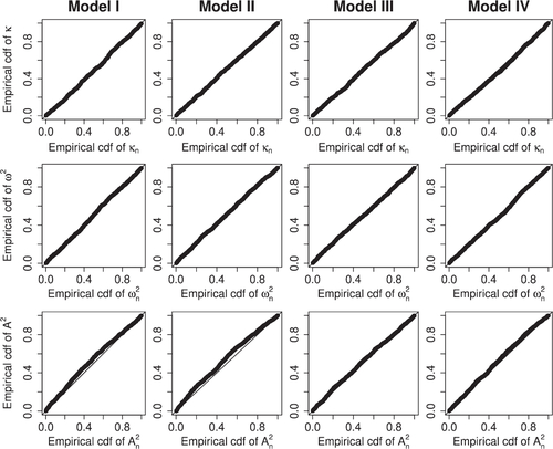
Table 1 Number of rejections in 1000 repetitions at 5% significance level.

	Model I	Model II	Model III	Model IV
κ n	36	49	41	38
${\omega }_n^2$	47	50	41	53
$A_n^2$	47	63	49	60

6.2 Simulations Under the Alternative Hypothesis

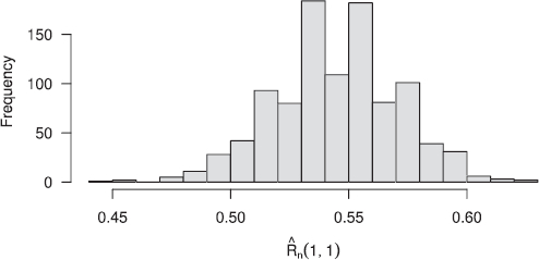
Before describing the simulation models under the alternative, we first note that the estimation of R(x, y) is statistically difficult in the sense that generally the corresponding estimator has considerable bias and variance. For simplicity, consider R(1, 1), the upper tail dependence coefficient. For the sample sizes used in this simulation section, it is hard to distinguish between the values $R(1,1)=0.5$ and $R\prime (1,1)=0.6$, say, so a test cannot achieve a high power in such a case. In order to substantiate this, we reuse the simulation results from the df F with the Clayton(1) survival copula and Pareto(3) margins in Model III above. In this case $R(1,1)=0.5$. The histogram in Figure 2 depicts the distribution of the 1000 estimates ${\widehat{R}}_n(1,1)$. The (empirical) bias of these estimates is as high as 0.046 and the sample standard deviation is 0.026. We see from the figure that the central 95% of the estimates range from 0.492 to 0.596; the true value is barely included in this interval and the range is rather wide. Note that when performing a two-sample test, the bias and variance of the second sample also have to be taken into account.

Fig. 2 Histogram of ${\widehat{R}}_n(1,1)$ values computed from 1000 bivariate samples with Clayton(1) survival copula and Pareto(3) margins.

In this section, we consider the four models listed below. The linear factor model of Model IVa refers to the bivariate random vector(18) $$(\lambda Z_1+(1-\lambda )Z_2,\mu Z_1+(1-\mu )Z_2),$$(18) with Z₁, Z₂ independent and $\lambda ,\mu \in (0,1)$ deterministic parameters.

Model 1a.F has Gumbel(2) copula and Pareto(3) margins, $F\prime$ has Gumbel(6) copula and Pareto(4) margins.

Model IIa.F has Gumbel(4) copula and Pareto(3) margins, $F\prime$ has Gumbel(1) (i.e., independence) copula and Pareto(4) margins.

Model IIIa.F has Clayton(1) survival copula and Pareto(3) margins, $F\prime$ has Clayton(5) survival copula and Pareto(4) margins.

Model IVa.F is the df of the linear factor model (18), with $Z_1,Z_2\sim \text{Pareto}(1),\lambda =0.9,\mu =0.8$, and $F\prime$ is the df of the same model (18) with $Z_1,Z_2\sim \text{Pareto}(2),\lambda =0.9,\mu =0.2$.

As in Section 6.1, we construct PP-plots for each model and each of the three test statistics; see Figure 3. The PP-plots show dramatic deviations from the behavior under a standard Wiener process. We also present rejection counts at 5% significance level in Table 2. As suggested by the PP-plots, the three omnibus tests have high power with, for the present alternatives, Cramér-von Mises outperforming Kolmogorov-Smirnov, and Anderson-Darling performing the best. Based on this, we recommend to apply both the Cramér-von Mises and the Anderson-Darling type test statistics.

Fig. 3 PP-plots for the three test statistics constructed from 1000 simulated sample pairs per model.

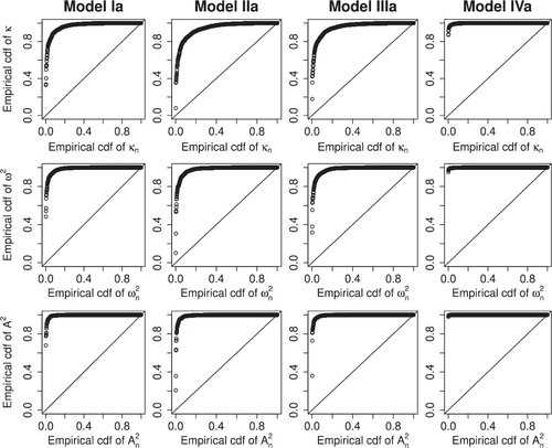
Table 2 Number of rejections in 1000 repetitions at 5% significance level.

	Model Ia	Model IIa	Model IIIa	Model IVa
κ n	836	704	778	994
${\omega }_n^2$	922	896	891	1000
$A_n^2$	977	963	974	1000

In Figure 4, we also provide empirical power curves at 5% significance level for the three test statistics, computed from a sequence of eight models similar to Model Ia. In each model, F has Gumbel(θ) copula and Pareto(3) margins, $F\prime$ has Gumbel(6) copula and Pareto(4) margins, and θ takes a sequence of values in the interval (1, 6) so that the difference of the tail dependence coefficients $R\prime (1,1)-R(1,1)$ takes a sequence of values ranging from 0.1 to 0.8. Observe that the power grows quickly and is high as soon as the difference is 0.2. The exact values of θ that were used, and the corresponding differences $R\prime (1,1)-R(1,1)$, can be seen in Table 3. Each point in a given power curve represents the observed rejection rate at the 5% level among 200 sample pairs.

Fig. 4 Empirical power curves for the three test statistics, constructed from a sequence of eight models similar to Model Ia.

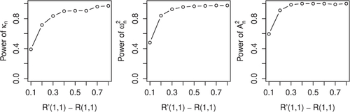
Table 3 Gumbel parameter values used for the empirical power curves, and the corresponding differences $R\prime (1,1)-R(1,1)$.

θ	3.45	2.48	1.97	1.65	1.43	1.27	1.15	1.06
$R\prime (1,1)-R(1,1)$	0.1	0.2	0.3	0.4	0.5	0.6	0.7	0.8

7 Empirical Analysis

Emboldened by the Monte Carlo simulation results of the previous section, demonstrating good size and power performances, we now take our approach to real equity index data of three financial markets. We take $\delta =0.25$, T = 2 and ${\overline{c}}_n(x,y)=\overline{c}{\prime }_{n\prime }(x,y)={\tilde{c}}_n(x,y)=\tilde{c}{\prime }_{n\prime }(x,y)=1.5$ as in Section 6, and consider a range of k-values (see below).

An important concern when analyzing multiple financial markets operating in different time zones is the synchronicity of the data, which requires a careful treatment. We use intra-daily data to construct three synchronized time series of daily equity index returns: for FTSE 100 (UK), DAX 30 (Germany), and S&P 500 (US). Data are obtained from the Tick History Database of Thomson Reuters. Our full sample spans the period May 2008 to August 2015. Using Coordinated Universal Time (UTC), care has been taken to account for the change to Daylight Savings Time (DST), which does not occur on the same day around the world.

We focus on the pair {FTSE 100, DAX 30} for a detailed exposition. We construct two bivariate samples from the daily negative log-returns of these two indices: the first sample is generated from the 900 trading days preceding January 1, 2012 (spanning the period from May 23, 2008 to December 31, 2011), and the second sample is generated from the 900 trading days following January 1, 2012 (spanning the period from January 1, 2012 to August 13, 2015). To be more precise, the daily negative log-returns for a given index are the numbers $\hspace{0.17em}\log \hspace{0.17em}(p_t/p_{t+1})$, with p_t denoting the index price recorded at 14:30 UTC (13:30 UTC during European DST) on trading day t. Note that the first sample covers some of the most volatile trading days of the global financial crisis and the subsequent European debt crisis, while the second sample can be considered a relatively calm “post-crisis” period. We aim to test whether or not the tail dependence structure in the two samples, as characterized by the tail copula, shows statistical evidence of a change. As an interesting alternative analysis, which we will not pursue here, one could compare the tail copulas associated with the upper and lower tails of the daily bivariate log-returns within the same sampling period. Indeed, these bivariate extremal gains can be seen to be asymptotically independent of the bivariate extremal losses.

Figure 5 displays plots of the daily negative log-returns for the two indices during the two time periods, and Table 4 provides some sample statistics for these time series. It is visibly clear that the marginal structure changes for both indices from period 1 to period 2, but a possible change in the tail dependence structure is much more difficult to detect by visual inspection. The change in the marginal structure can also be observed in Figure 6, which plots the estimated extreme value index γ for each marginal dataset over a set of k values ranging from 100 to 200. It is clear that the (right) tail of the daily negative log-returns is heavier in the first period (with EV index estimates firmly positive) than in the second period (with EV index estimates mostly hovering below 0).

Fig. 5 Daily negative log-returns of FTSE 100 (top) and DAX 30 (bottom) in the two periods. Tick marks on the horizontal axes indicate the first trading day of each year.

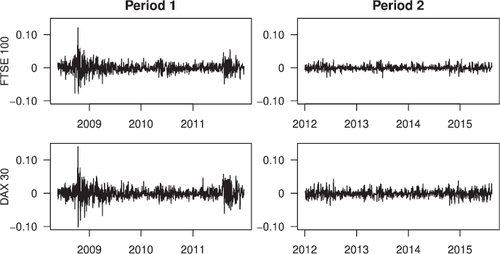
Fig. 6 Estimated marginal extreme value indices of the daily negative log-returns of FTSE 100 and DAX 30 in the two periods.

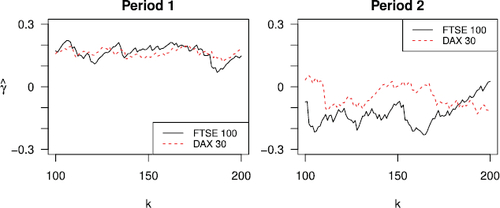
Table 4 Sample statistics of the daily negative log-returns of FTSE 100 and DAX 30 in the two periods.

	Period 1
	Mean	SD	Min	Max
FTSE 100	0.000	0.016	–0.078	0.121
DAX 30	0.000	0.019	–0.102	0.140
Period 2
Mean	SD	Min	Max
0.000	0.008	–0.030	0.028
0.001	0.011	–0.037	0.043

The next step in our analysis is to transform the observed negative log-returns (X_i, Y _i) in period 1 and $(X{\prime }_i,Y{\prime }_i)$ in period 2 into $({\widehat{X}}_i,{\widehat{Y}}_i)$ and $(\widehat{X}{\prime }_i,\widehat{Y}{\prime }_i)$ as described in (5), which leads to estimates ${\widehat{R}}_n$ and $\widehat{R}{\prime }_n$ of the tail copulas R and $R\prime$ in the two periods. Figure 7 displays scatterplots of the transformed negative log-returns in the two periods, for k = 150. Since the transformation (5) maps joint extremes (X_i, Y _i) to points near the origin, the tail copula estimate ${\widehat{R}}_n(x,y)$ is proportional to the number of points $({\widehat{X}}_i,{\widehat{Y}}_i)$ inside the rectangle $[0,x]\times [0,y]$ (and analogously for $\widehat{R}{\prime }_n$). In particular, the upper tail dependence coefficients R(1, 1) of period 1 and $R\prime (1,1)$ of period 2 can be estimated by dividing the number of points $({\widehat{X}}_i,{\widehat{Y}}_i)$ or $(\widehat{X}{\prime }_i,\widehat{Y}{\prime }_i)$ in ${[0,1]}^2$ by k. This leads to estimates ${\widehat{R}}_n(1,1)=115/150=0.77$ and $\widehat{R}{\prime }_n(1,1)=104/150=0.69$. The difference is small, and, also in light of the estimator’s substantial bias and variance illustrated in Figure 2 for simulated data, it is not at all clear if it indicates a difference in the true tail copulas R and $R\prime$. Also note that R(1, 1) does not tell the whole story about tail dependence, which can only be properly described by the entire tail copula R.

Fig. 7 Transformed daily negative log-returns $({\widehat{X}}_i,{\widehat{Y}}_i)$ of period 1 and $(\widehat{X}{\prime }_i,\widehat{Y}{\prime }_i)$ of period 2, with k = 150. The number of points in the square ${[0,1]}^2$, divided by k, gives the estimates ${\widehat{R}}_n(1,1)=115/150=0.77$ and $\widehat{R}{\prime }_n(1,1)=104/150=0.69$.

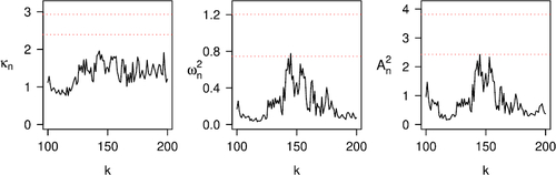
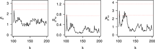
It remains to construct the test process W_n and compute the test statistics in (17), as in Section 6. We do this again for $k=100,\dots ,200$. Plots of the resulting test statistics can be seen in Figure 8, together with the 95th and the 99th percentiles of their distributions under the null hypothesis. Each test statistic stays below the 95th percentile of the corresponding null distribution essentially for the entire range of k values, leading to non-rejection of the null hypothesis. Thus, the conclusion based on these three test statistics is that the tail dependence structure between the daily negative log-returns of FTSE 100 and DAX 30 does not change from period 1 to period 2, despite the visible evidence of change in the marginal (tail) behaviors of both equity indices.

Fig. 8 The three test statistics in (17) computed from the daily negative log-returns of FTSE 100 and DAX 30 in periods 1 and 2. The dotted lines indicate the 95th and 99th percentiles of the corresponding null distributions.

For an independent verification, we also apply the multiplier bootstrap test for the equality of tail copulas described in Bücher and Dette (2013) to our dataset. An implementation of the partial derivative multiplier (pdm) approach, as outlined in Section 4.1 of that paper, with k = 150 and 500 bootstrap replications, leads to an estimated p-value of 0.42 for the null hypothesis of equal tail copulas, which is consistent with our conclusion.

A possible objection against this application could be that, per period, the data may be serially dependent. First note that pairwise dependence in the tails can only be “positive”; for example, for the countermonotonic copula, the case of perfect negative dependence, the corresponding tail copula is just the 0-function, the same as for the independence copula. Loosely speaking, in case of (positive) serial dependence at high levels, the data contain less information about the underlying df than in the iid case. Hence, estimation errors, that is, variances, become larger and so do therefore the critical values of the tests. As a result, our tests can, in fact, be considered as anticonservative (that is, they overreject): if the null hypothesis is not rejected under the iid assumption, it will not be rejected when serial dependence is taken into account. In the Appendix, we provide some empirical support for this heuristic argument via simulations: rerunning Model III of Section 6.1 with component-wise serial dependence in both samples leads to higher rejection rates as expected. So, our conclusion of no change in tail copulas remains.

Having considered the tail dependence between a pair of European equity indices, we now turn our attention to the tail dependence between the transatlantic pair {FTSE 100, S&P 500}. We compute, like above, the daily negative log-returns of these two indices during the same periods 1 and 2 defined earlier, using daily synchronous index price data recorded at 14:30 UTC (13:30 UTC during European DST). Figure 9 displays plots of the daily negative log-returns for the two indices during the two time periods, and Table 5 provides sample statistics. As before, we see clear evidence of a change in the marginal behavior of the negative log-returns in period 1 versus in period 2.

Fig. 9 Daily negative log-returns of FTSE 100 (top) and S&P 500 (bottom) in the two periods. Tick marks on the horizontal axes indicate the first trading day of each year.

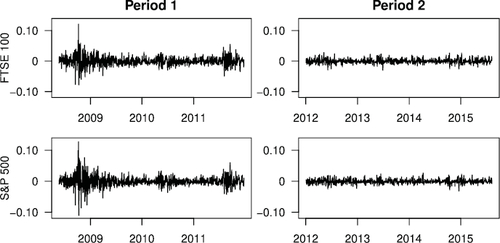
Table 5 Sample statistics of the daily negative log-returns of FTSE 100 and S&P 500 in the two periods.

	Period 1
	Mean	SD	Min	Max
FTSE 100	0.000	0.016	–0.078	0.121
S&P 500	0.000	0.018	–0.111	0.127
Period 2
Mean	SD	Min	Max
0.000	0.008	–0.030	0.028
0.001	0.007	–0.032	0.027

To test if there is a change in the tail dependence structure, we again construct our test process W_n from the two bivariate samples generated from the two periods, and compute the three test statistics in (17) for $k=100,\dots ,200$; see Figure 10. We find that each test statistic mostly stays below the 95th percentile of the corresponding null distribution, with a few exceptions at particular k values. Keeping in mind that (i) looking at several k values simultaneously amounts to a multiple testing problem, and (ii) our datasets likely feature some serial dependence, both of which have an upward effect on critical values for the test statistics, we conclude that our testing approach again supports the null hypothesis of no change in the tail dependence structure of the negative log-returns in period 1 versus in period 2.

Fig. 10 The three test statistics in (17) computed from the daily negative log-returns of FTSE 100 and S&P 500 in periods 1 and 2. The dotted lines indicate the 95th and 99th percentiles of the corresponding null distributions.

As with the earlier dataset of {FTSE 100, DAX 30} negative log-returns, we also apply the pdm bootstrap test of Bücher and Dette (2013) to the present dataset, with k = 150 and 500 bootstrap runs. This leads to an estimated p-value of 0.38 for the null hypothesis of equal tail copulas, which is again consistent with our conclusion.

8 Conclusions

We have developed a novel, general procedure to test for the equality of the tail copulas associated with two samples of bivariate data. A natural but complex feature of this problem is that the tail copulas, of which equality is tested for, are not specified. Deploying a martingale transformation of the suitably normalized difference between two semiparametric estimators of the tail copulas, we have constructed a two-sample hypothesis testing process and established its weak convergence to a standard Wiener process under the null hypothesis. Applying our hypothesis testing procedure to samples of negative log-returns of equity indices, during and after the global financial crisis, we find no evidence to reject the null hypothesis of tail copula equality. That is, although large negative returns occur more frequently and severely during crisis versus post-crisis for the pairs of equity indices we have analyzed, our testing procedure reveals that there is no statistical evidence of a change in their tail dependence structure. These findings suggest that, for the highly developed equity markets we consider, whereas inference about marginal (tail) behavior should account for changes over time or across “regimes,” the tail dependence structure appears to be more stable and can thus be inferred from longer time periods.

Acknowledgments

We are very grateful to the Editor Professor Ivan Canay, the Associate Editor, and two referees for many useful comments that greatly improved the article. We also thank Estate V. Khmaladze for stimulating discussions about this article.

Supplementary Materials

Appendix:Proofs of Theorems 3.1, 4.1, 5.1; simulation results under serial dependence. (.pdf file)

Code: R code that implements our testing procedure. (.R file)

Disclosure Statement

The authors report that there are no competing interests to declare.

Additional information

Funding

John Einmahl holds the Arie Kapteyn Chair 2019–2022 and gratefully acknowledges the corresponding research support. Roger Laeven is supported in part by the Netherlands Organization for Scientific Research under an NWO-Vici grant 2020–2025.

References

- Beirlant, J., Goegebeur, Y., Teugels, J., and Segers, J. (2004), Statistics of Extremes: Theory and Applications, New York: Wiley.
- Bekaert, G., Harvey, C. R., and Ng, A. (2005), “Market Integration and Contagion,” The Journal of Business, 78, 39–69.
- Bekaert, G., Hodrick, R. J., and Zhang, X. (2009), “International Stock Return Comovements,” The Journal of Finance, 64, 2591–2626.
- Bormann, C., and Schienle, M. (2020), “Detecting Structural Differences in Tail Dependence of Financial Time Series,” Journal of Business & Economic Statistics, 38, 380–392.
- Bücher, A., and Dette, H. (2013), “Multiplier Bootstrap of Tail Copulas with Applications,” Bernoulli, 19, 1655–1687.
- Bücher, A., Jäschke, S., and Wied, D. (2015), “Nonparametric Tests for Constant Tail Dependence with an Application to Energy and Finance,” Journal of Econometrics, 187, 154–168.
- Can, S. U., Einmahl, J. H. J., Khmaladze, E. V., and Laeven, R. J. A. (2015), “Asymptotically Distribution-Free Goodness-of-Fit Testing for Tail Copulas,” Annals of Statistics, 43, 878–902.
- Christoffersen, P., Errunza, V. R., Jacobs, K., and Langlois, H. (2012), “Is the Potential for International Diversification Disappearing? A Dynamic Copula Approach,” The Review of Financial Studies, 25, 3711–3751.
- de Haan, L., and Ferreira, A. (2006), Extreme Value Theory: An Introduction, New York: Springer.
- de Haan, L., and Resnick, S. I. (1977), “Limit Theory for Multivariate Sample Extremes,” Zeitschrift für Wahrscheinlichkeitstheorie und Verwandte Gebiete, 40, 317–337.
- Delgado, M. A., Hidalgo, J., and Velasco, C. (2005), “Distribution Free Goodness-of-Fit Tests for Linear Processes,” Annals of Statistics, 33, 2568–2609.
- Draisma, G., Drees, H., Ferreira, A., and de Haan, L. (2004), “Bivariate Tail Estimation: Dependence in Asymptotic Independence,” Bernoulli, 10, 251–280.
- Einmahl, J., de Haan, L., and Sinha, A. (1997), “Estimating the Spectral Measure of an Extreme Value Distribution,” Stochastic Processes and Their Applications, 70, 143–171.
- Forbes, K. J., and Rigobon, R. (2002), “No Contagion, Only Interdependence: Measuring Stock Market Comovements,” The Journal of Finance, 57, 2223–2261.
- Joe, H. (2001), Multivariate Models and Dependence Concepts (2nd ed.), Boca Raton, FL: Chapman & Hall/CRC.
- Khmaladze, E. V. (1981), “Martingale Approach in the Theory of Goodness-of-Fit Tests,” Theory of Probability and its Applications, 26, 240–257.
- Khmaladze, E. V. (1988), “An Innovation Approach to Goodness-of-Fit Tests in Rm,” Annals of Statistics, 16, 1503–1516.
- Khmaladze, E. V. (1993), “Goodness of Fit Problem and Scanning Innovation Martingales,” Annals of Statistics, 21, 798–829.
- Khmaladze, E. V., and Koul, H. L. (2004), “Martingale Transforms Goodness-of-Fit Tests in Regression Models,” Annals of Statistics, 32, 995–1034.
- King, M. A., and Wadhwani, S. (1990), “Transmission of Volatility between Stock Markets,” The Review of Financial Studies, 3, 5–33.
- Koenker, R., and Xiao, Z. (2002), “Inference on the Quantile Regression Process,” Econometrica, 70, 1583–1612.
- Koenker, R., and Xiao, Z. (2006), “Quantile Autoregression,” Journal of the American Statistical Association, 101, 980–990.
- Kotz, S., and Nadarajah, S. (2000), Extreme Value Distributions: Theory and Applications, London: Imperial College Press.
- Longin, F., and Solnik, B. (1995), “Is the Correlation in International Equity Returns Constant: 1960–1990?” Journal of International Money and Finance, 14, 3–26.
- Towghi, N. (2002), “Multidimensional Extension of L.C. Young’s Inequality,” Journal of Inequalities in Pure and Applied Mathematics, 3, 1–30.